Uncertainties in LCA (Subject editor: Andreas Ciroth)
Using Standard Statistics to Consider Uncertainty in Industry-Based
Life Cycle Inventory Databases
Hirokazu Sugiyama1,2*, Yasuhiro Fukushima2, Masahiko Hirao2, Stefanie Hellweg1 and Konrad Hungerbühler1
1 Institute for Chemical and Bioengineering, Swiss Federal Institute of Technology, ETH Hönggerberg, 8093 Zurich, Switzerland 2 Department of Chemical System Engineering, The University of Tokyo, 7-3-1 Hongo, Bunkyo-ku, 113-8656 Tokyo, Japan
* Corresponding author (hirokazu.sugiyama@chem.ethz.ch)
for the case study, the uncertainty distribution of the LCA result is hypothetical. However, the merit of adopting the proposed procedure has been illustrated: more informed decision-making becomes possible, basing the decisions on the significance of the LCA results. With this illustration, the authors hope to encour-age both database developers and data suppliers to incorporate uncertainty information in LCI databases.
Keywords:Decision making; Life Cycle Inventory (LCI) data-bases; Maximum Likelihood Estimation (MLE) method; Monte Carlo simulation; PET chemical recycling; rank order correla-tion coefficient; statistics; uncertainty analysis
DOI: http://dx.doi.org/10.1065/lca2005.05.211 Abstract
Goal, Scope and Background. Decision-makers demand infor-mation about the range of possible outcomes of their actions. Therefore, for developing Life Cycle Assessment (LCA) as a decision-making tool, Life Cycle Inventory (LCI) databases should provide uncertainty information. Approaches for incor-porating uncertainty should be selected properly contingent upon the characteristics of the LCI database. For example, in indus-try-based LCI databases where large amounts of up-to-date proc-ess data are collected, statistical methods might be useful for quantifying the uncertainties. However, in practice, there is still a lack of knowledge as to what statistical methods are most effective for obtaining the required parameters. Another con-cern from the industry's perspective is the confidentiality of the process data. The aim of this paper is to propose a procedure for incorporating uncertainty information with statistical meth-ods in industry-based LCI databases, which at the same time preserves the confidentiality of individual data.
Methods. The proposed procedure for taking uncertainty in in-dustry-based databases into account has two components: con-tinuous probability distributions fitted to scattering unit proc-ess data, and rank order correlation coefficients between inventory flows. The type of probability distribution is selected using statistical methods such as goodness-of-fit statistics or experience based approaches. Parameters of probability distri-butions are estimated using maximum likelihood estimation. Rank order correlation coefficients are calculated for inventory items in order to preserve data interdependencies. Such prob-ability distributions and rank order correlation coefficients may be used in Monte Carlo simulations in order to quantify uncer-tainties in LCA results as probability distribution.
Results and Discussion. A case study is performed on the tech-nology selection of polyethylene terephthalate (PET) chemical recycling systems. Three processes are evaluated based on CO2
reduction compared to the conventional incineration technol-ogy. To illustrate the application of the proposed procedure, assumptions were made about the uncertainty of LCI flows. The application of the probability distributions and the rank order correlation coefficient is shown, and a sensitivity analysis is performed. A potential use of the results of the hypothetical case study is discussed.
Conclusion and Outlook. The case study illustrates how the un-certainty information in LCI databases may be used in LCA. Since the actual scattering unit process data were not available
Introduction
New Life Cycle Inventory (LCI) and Life Cycle Assessment (LCA) databases, such as the ecoinvent database [1,2] from Switzerland or JLCA-LCA database [3,4] from Japan, have recently been published. Covering a wide range of industry, representative unit process data on a national level (e.g. whole Japan) or regional level (e.g. Europe) have become avail-able. In this paper, the term unit process data refers to the amount of input and output flow to produce a unit amount of product in an industrial process step. Concerning the un-certainty of unit process data, the ecoinvent database pro-vides probability distributions of inventory data for most of the processes while the current version of the JLCA-LCA database does not include uncertainty information. Ap-proaches for incorporating uncertainty should be selected appropriately because data development procedure is dif-ferent from database to database. In ecoinvent database, for example, literature is the major basis. Therefore, the reli-ability of source data itself or inequality in scope between source data and the database (e.g. temporal or geographical gaps) is likely the major source of uncertainty. For this rea-son, in literature-based LCI databases, approaches that can quantify qualitative sources of uncertainty, such as the Pedi-gree Matrix approach [5], are important. Conversely, in in-dustry-based LCI databases, up-to-date process data is often available and statistical methods might come into play. For the JLCA-LCA database, major industrial associations collect the most current gate-to-gate data from member companies and process their own data statistically with a critical review according to a guidance manual supplied by the database de-veloper, JLCA. Each association reports unit process data,
averaged over factories, to the database developer. Individual unit process data and copyrights of the data remain with the corresponding industrial associations. Thus, statistical data treatment is left up to the individual association.
For the JLCA-LCA database, the developer has attempted to represent uncertainty by minimum and maximum values: the guidance manual asks each industry association to re-port minimum and maximum values of unit process data among comparable factories. However, this procedure has two major problems. One is that the deviation of the origi-nal distribution is not retrieved. For example, when very small or large values are minimum or maximum values, while most of the data points are centralized near mean value, such deviation cannot be reconstructed later. Another con-cern is that interdependencies of unit process data are not considered. Although industry associations have a large number of data points at their disposal, information such as deviation and interdependencies are lost in the current pro-cedure. Another aspect in regard to industry data intensive databases is the confidentiality of the data. It is very impor-tant for industry that the bare industrial data is not pub-lished, but masked in the database. For example, experts in competing companies may detect which technology is in-volved in the other companies merely through anonymous data. As a result, in the case of the JLCA-LCA database, industrial associations have not, thus far, reported minimum and maximum values, since they are optional.
In order to palliate these shortcomings, we propose a data treatment procedure for industry-based LCI databases. The main aim of this article is to clarify (a) which statistical pa-rameters should be obtained and (b) how classical statistics should be used to derive these parameters in industry-based LCI databases. This method also preserves the confidential-ity of the individual data. Continuous probabilconfidential-ity distribu-tions are fitted to the scattering individual unit process data. Correlation coefficients are used to represent interdependen-cies. The unit process data is described by probability dis-tributions and correlation coefficients, which can be directly used in Monte Carlo simulations for overall LCI and LCA calculations. In a case study involving polyethylene terephthalate (PET) chemical recycling systems, we show how the presented uncertainty information can be used in LCA, thereby contributing to more informed decision-making.
1 Procedure for Considering Uncertainty in LCI Databases 1.1 Conventional method of reporting deterministic data in
LCI databases
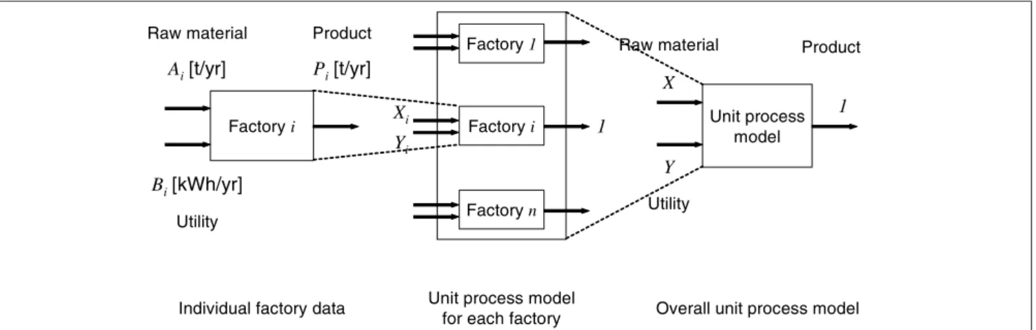
Fig. 1 illustrates a hypothetical situation in which an
'over-all unit process model' is created. This model includes fac-tories producing the same product in the scope or the sponding region of the LCI database. This activity corre-sponds to the aggregating phase in the PHASETS (PHASES in the design of a model of a Technical System) procedure proposed by Carlson and Pålsson [6], where the same tech-nical system is averaged. 'Individual factory data' is assumed to be obtained as raw material Ai [t/yr], utility input Bi [kWh/
yr] and product output Pi [t/yr] for factory i. A linear
rela-tion is assumed between input and output flows (Eq. 1): (1) The value of the parameters Xi and Yi can be scattering over
factories. Hanssen and Asbjørnsen have shown such differ-ent unit process data from 26 pulp production sites in Swe-den [7]. Huijbregts discussed and categorized sources of such uncertainty [8]. Ciroth et al. further discussed the relation-ship between geographical and technological differences in unit process data [9]. In this paper, the sources of the scat-tering are not discussed further. The focus lies in the data treatment after obtaining scattering industrial data. One common way to determine X and Y, the parameters of the 'overall unit process model', is to use weighted averages based on the market share, as displayed in Eq. 2.
(2)
where wi is the market share of factory i to the whole
pro-duction amount, and n is the number of factories inside the database scope. This approach is often followed in conven-tional LCI databases. Information of scattering data is obvi-ously lost. Ideally, the parameter X, for example, can be presented as a discrete function using the individual values
Ai[t/yr] Bi[kWh/yr] Factory i Pi[t/yr] Product Raw material Utility
Individual factory data
Factory i Factory 1
Factory n
Unit process model
Unit process model for each factory Xi
Yi 1
X
Y
1
Overall unit process model Raw material
Utility
Product
Rank Order
Correlation Coefficient rX-Y
Fitting by Maximum Likelihood Estimation method Scattering plot of (Xi, Yi) X = LogNormal Y = Nor m al
of Xi and wi. However, as mentioned before, it is often diffi-cult to publish such individual data in LCI databases due to confidentiality reasons (see Fig. 1).
1.2 New procedure for including uncertainty information in industry-based LCI databases
The proposed procedure is comprised of two components: the first is fitting continuous probability distributions to Xi and Yi (Fig. 2). Fitting continuous distributions is employed for the purpose of masking bare unit process data in each factory. After specifying the type of distribution, the charac-teristic parameters of the distribution (e.g. mean, standard deviation) are estimated using the Maximum Likelihood Estimation (MLE) method [10,11]. The second component is a correlation coefficient between Xi and Yi. Such correla-tions are represented by the rank order correlation coeffi-cient [11]. Derivation of these components is described in detail in the following sections.
The merits of this approach within LCA are the following: (a) It facilitates Monte Carlo simulations, which are simple, can manage every kind of distributions, and can be used with any kind of operation [12]. (b) Monte Carlo simulations are increasingly applied in LCA, e.g. [13–15]. (c) LCA soft-ware has started implementing this approach (e.g. GaBi 4 [16] or Sima Pro 6 [17]). A more detailed comparison of Monte Carlo simulations with other uncertainty propaga-tion approaches is presented by Ciroth et al. [18].
tribution among a set of candidates [11]. In cases where few data points are available, expert judgment may be needed. Maurice et al. have proposed the use of uniform, triangular and pert distributions (derived from beta distribution), which have a limited range [12]. Ecoinvent, in its current version, uses lognormal distributions for all unit process data [1,2]. After specifying the type of probability distribution, the char-acteristic parameters of the distribution should be estimated. We propose the use of the MLE method, which is the most common technique used to fit distributions to available data sets [11]. The maximum likelihood estimators of a distribu-tion are the values of its parameters that produce the maxi-mum joint probability density for the observed data. Con-sider a probability distribution type defined by a single parameter, α. The likelihood function L(α) is proportional to the probability that a set of n data points Xi could be
generated from the distribution with probability density f(X) and given by Eq. 3
(3)
For incorporating the market share wi, the likelihood func-tion is modified and redefined as (Eq. 4)
(4) where N is an arbitrary number such as 1000, which is large enough to make Nwi an integer. Technically, Xi is treated as quasi Nwi numbers of data points. For example, Xj, with 35.2%
market share wj, is treated as 352 data points of Xj when N is
1000. By having the power term Nwi, values of Xi with a larger market share receive more weight and vice versa. The
maximum likelihood estimator is then the value of α that
maximizes L(α). It is determined by taking the partial differ-ential of L(α) with respect to α and setting it to zero [11] (Eq. 5). (5)
Estimated parameters depend on the type of the distribution. For example, in the case of normal or lognormal distribution, both mean and standard deviation determine the property of the distribution and become maximum likelihood esti-mators. When normal distribution or lognormal distribu-tion is fitted to X, Y in the example of Fig. 1, MLE provides the mean and standard deviation, which then define the dis-tribution. For example, X can be expressed as (Eq. 6),
(6) where the mean value µX is equivalent to the value in Eq. (2). The fittings based on MLE and GOF statistics are avail-able in commercial software (e.g. BESTFIT [19]).
Fig. 2: Two components of the proposed procedure: probability distribu-tion using the Maximum Likelihood Estimadistribu-tion (MLE) method and rank order correlation coefficient
1.2.1 Fitting probability distributions and estimating characteristic parameters by the Maximum Likelihood Estimation (MLE) method
There is no established rule for fitting probability distribu-tions on scattering individual unit process data. However, several suggestions are found in literature. Hanssen and Asbjørnsen have analyzed unit process data from 26 pro-duction sites and found that binominal distributions can best estimate process emissions (e.g. SO2 emission per product) [7]. If more than 30 data points are available, goodness-of-fit (GOF) statistics can assist in identifying the best-goodness-of-fit
dis-1.2.2 Preserving interdependency of inventory items by rank order correlation coefficient
In order to preserve interdependencies of inventory items, we propose the use of Spearman's rank order correlation coefficient (Eq. 7) [11].
(7) Here again, it is assumed that a number of Nwi data points
have the value of Xi, and Yi. rank(Xi) is the rank among the
N tuple data points. For example, X1, the largest among all
X, is treated as Nw1 numbers of points with rank 1. X2, the
second largest, is treated as Nw2 points with rank 1 + Nw1.
As seen in Eq. 7, if Xi and Yi have the same rank for every i,
the correlation coefficient becomes 1. The use of rank order correlation coefficient instead of regression correlation co-efficient makes it possible to generate correlated variables from two probability distributions in the Monte Carlo simu-lation; numbers which were once generated independently are transformed to desired distributions preserving rank or-der correlation coefficient [20]. This algorithm is imple-mented in commercial software, e.g. @RISK® [19], which is
an add-in software to MS-EXCEL®.
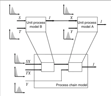
1.3 Unit process model to process chain model
The LCI can be calculated by creating process chain mod-els. A simple example is shown in Fig. 3, where the product of process B is the raw material of the process A. The pa-rameters of each unit process, normalized by its product amount, are described by probability distributions and cor-relation coefficients. Using the product amount of process A as a functional unit, the overall input (SX, TX and Y) can be calculated by using Monte Carlo simulation.
2 Case Study
2.1 Definition of the goal and scope
The goal of the case study is to illustrate the application of our procedure in the previous section. Emphasis is placed on highlighting the benefits of our procedure, rather than on the numerical facts. The intended decision-maker is, for
example, a (local) government that wants to reduce CO2
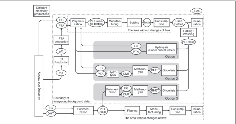
emissions by introducing a PET chemical recycling process with 1,000 t/yr capacity. Recycling options in the PET prod-uct life cycle are shown in Fig. 4. The functional unit of the study is 1,000 t/yr of used PET bottles. In this hypothetical case, we assume that the significance level is desired as 90% by the (local) government. The life cycle CO2 emissions are compared before and after the installation of the recycling plant; i.e. the base case is the current condition, in which used bottles are incinerated with electricity generation at 10% thermal efficiency. Among emissions through the life cycle of PET bottles, CO2, NOX, SOX are major contribut-ing emissions within the Eco Indicator 99 method [21], us-ing the LCI dataset 'PET, bottle grade, at plant (RER)' of the ecoinvent database [22]. In this work, CO2 is taken as a
reduced environmental metric because CO2, NOX and SOX
are emitted in conjunction (e.g. in fuel consumption). For the purposes of this study, namely the illustration of the method presented in Section 2, the assessment of CO2 is suf-ficient, as other environmental metrics could be calculated in a similar way. In each option, 1,000 t/yr of used PET are supplied to recycling processes after pre-treatment in con-ventional flaking processes.
For the inventory analysis, existing unit processes are modeled using previous studies for PET products [23–25]. Unit processes inside the single dotted line in Fig. 4 are modeled with input and output flows, while the ones
out-side the line are modeled using cumulative CO2 emission
factors; i.e. total CO2 amount emitted for providing the prod-uct up to the dotted line. Chemical recycling processes are
modeled using the chemical process simulator HYSYS® [26]
with information from literature [27–29] or corresponding industry. CO2 emissions in each option or the base case are calculated using Eq. 8, and changes of CO2 emissions from the base case are calculated with Eq. 9.
(8)
(9)
Ω(CO2) are the CO2 emissions from the life cycle systems (the whole system in Fig. 4) for i: option 1–3 or the base case. Out(CO2) are the CO2 emissions occurring directly from the system (single dotted line). a and b refer to mate-rial or energy. In and Out are inputs and outputs to and
from the boundary, and ϕ is the cumulative CO2 emission
Unit process model A Y X 1 Unit process model B T S 1 Y 1 TX SX
Process chain model
Fig. 3: Creation of the process chain model from two unit process models. The product of the process B is the raw material for the process A. The parameters for the whole process chain models are normalized by the unit production amount of process A
- 6000 - 4000 - 2000 0 2000 4000 6000 Cha nge of CO 2 em is s ions [t ] option1 option2 option3 Recycling process Incineration Monomer production for PET bottles
Summation PET fiber production factor for the corresponding material or energy. p is a set of
parameters representing the uncertainty of unit processes data consisting of the type of probability distribution, pa-rameters for the distribution and correlation coefficients. 2.2 Uncertainty input information
In each of the foreground and existing processes (i.e. pX production, PTA production, incineration and flaking and washing processes), the amounts of utility consumption (e.g. electricity, steam and cooling water) were assumed to be log normally distributed. Reported data were used as mean val-ues. The coefficient of variation, i.e. the ratio of standard deviation to the mean value, was set to 0.5 for electricity, 0.3 for steam and 0.1 for cooling water. Within one unit process, rank order coefficients between utility consumptions were assumed to be 0.8. It is reasonable to assume a posi-tive correlation, because processes with better thermal effi-ciency tend to use less steam and cooling water. As an ex-ample, probability distributions in the primary PTA pro-duction are shown in Table 1. Additionally, transport
dis-tances are assumed to be triangle distributions, ranging ±50%
around the mean values [23,25]. For the cumulative CO2
emission factor of electricity, a discrete distribution is cre-ated based on the share of different production technologies [24]. No probability distribution is assumed on other cu-mulative CO2 emission factors.
2.3 LCA results and interpretation
Fig. 5 shows the deterministic values of ∆Ωi,BaseCase(CO2) for
option i (i = 1–3). On the one hand, CO2 is emitted from the recycling processes. On the other hand, however, the substi-tution of virgin material for bottles and fibers leads to a saving of CO2 emissions. CO2 emissions also decrease in the incineration process of PET bottles, because stopping incin-Fig. 4: Life cycle systems of PET products considering different options for chemical recycling processes. Abbreviation: pX refers to para xylene, mX to mixed xylene, BHET to bis(hydroxyethyl) terephthalate, DMT to dimethyl terephthalate and PTA to purified terephthalic acid
Utility demand Mean value unit Probability
distribution
Electricity from grid 0.651 kWh Lognormal,
CV=0.5 Middle pressure steam
from utility plant
0.848 kg Lognormal,
CV=0.3 Low pressure steam from
utility plant
0.848 kg Lognormal,
CV=0.3
cooling water 193 kg Lognormal,
CV=0.1
Table 1: Utility consumption in primary PTA production (excerpt from [23] normalized by 1 kg of PTA as a product)
Fig. 5: Changes of CO2 emission after installing recycling processes. The
eration of PET directly reduces the CO2 emissions. The sub-stitution of conventional electricity production through PET incineration is included in the graph. However, this increase is very small due to the low net calorific value of PET and the low energy recovery efficiency (10% in [23,25]). The summation indicates that all three recycling options reduce CO2 emissions. Option 1 is the most promising option; how-ever, it is very close to option 3. In such cases, uncertainty analysis becomes instrumental in evaluating the significance of the difference between the two alternatives.
Relative indicators help us to judge the significance of such differences [30]. This can be calculated as follows (Eq. 10); (10) In Fig. 6, the results of ∆Ωi, option 1(CO2) (i = option 2, 3) are
shown. The probability that option 1 becomes superior to option 3 can be calculated from the integration of the prob-ability distribution ∆Ωoption3,option1(CO2) above 0, which is
61%. Option 2 can be regarded as inferior to option 1 by 99%. If the decision-maker sets the significance level to 90%, option 2 can be rejected as promising for implementation. Option 3 may remain in the scope of comparison to be analyzed further. This illustrates that the deterministic analy-sis alone might have led to conclusions which are not statis-tically relevant. Conversely, after considering uncertainty, differences between options become more evident, enabling a more informed decision-making process. One prerequisite of such uncertainty analysis is an LCI database containing uncertainty information. Industry-based LCI databases can provide uncertainty information with the parameters and procedures proposed in this paper.
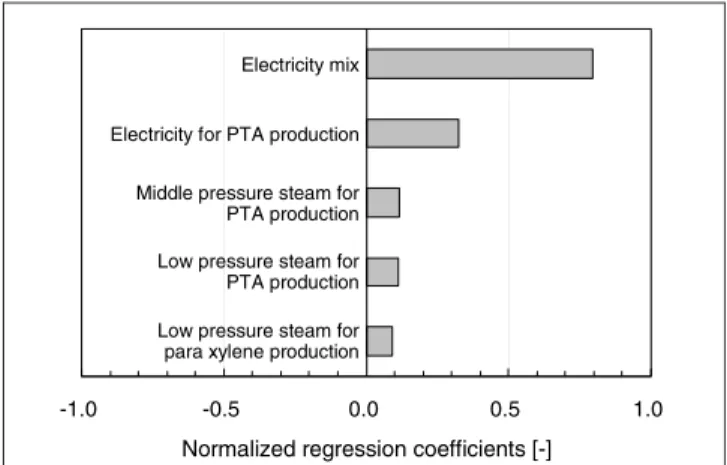
The contribution of each input uncertainty distribution to the cumulative uncertainty can be quantified by correlation coefficients between the values of each input distribution and the values of the output distribution. Because a linear model is used in this case study, multivariate stepwise re-gression method is used and normalized rere-gression coeffi-cients [20] are calculated. If the model is not linear, use of the rank order correlation coefficients is recommended [19]. Huijbregts et al. presented this correlation analysis as a sensi-tivity analysis, where input parameters are prioritized for fur-ther analysis [13]. Fig. 7 shows the five highest contributing
parameters for ∆Ωoption3,option1(CO2). The results show that the
discrete distribution of the CO2 emission factor dependent on the electricity mix contributes most to ∆Ωoption3,option1(CO2).
The coefficient value 0.8 of electricity mix means that a one standard deviation increase in the electricity mix increases ∆Ωoption3,option1(CO2) by 0.8 standard deviations. Thus, the
elec-tricity mix should be given priority in further analysis. A pos-sible refinement would be to check the latest emission factor, as the technology mix of electricity production changes from year to year. Another possibility would be to examine whether some processes use specific electricity sources. For example, less expensive nighttime electricity is usually dominated by nuclear electricity generation in Japan. The second contribu-tion comes from electricity consumpcontribu-tion in the primary PTA process, followed by other process data. Through these means of analysis, potential areas of improvement in the LCI model and data can be identified. This can be considered a further benefit of introducing uncertainty parameters in LCI databases. Parameters with larger absolute coefficient val-ues should get priorities for further analysis. In Fig. 7, we only show the parameters with coefficients larger than 0.08, because the contribution of all other parameters to the cu-mulative uncertainty is less than 10% of the contribution of the most influential parameter (electricity mix).
3 Conclusions
Drawing on the problems of the JLCA-LCA database, we have proposed a procedure for incorporating uncertainty information in industry-based LCI databases, using stand-ard statistical methods. The goal of our procedure is to sup-port industry-based LCI databases to incorporate scattering unit process data while retaining confidentiality in order to achieve more informed decision-makings in LCA. This pro-cedure has two components: fitting probability distributions to scattering data, and rank order correlation coefficients between interdependent LCI flows. This data can be directly applied in LCA using the Monte Carlo simulation. It is quite probable that problems similar to those in the JLCA-LCA database occur in other industry-based LCI databases (e.g. GaBi [16]). Therefore, the use of the proposed procedure is not limited to the JLCA-LCA database.
-1000 -500 0 500 1000 1500 2000 option2 option3 D if fer en ce of CO 2 e m issio n s re lat iv e to op tio n 1 [t ]
Fig. 6: Difference between options 2 and 3 and option 1(∆Ωi,option1(CO2),
i=option 2, 3) with indicators of 1%, 5%, mean, 95% and 99% points. Option 1 can be regarded as superior to option 3 at 61% probability by the integration of ∆Ωoption3,option1(CO2) above 1
-1.0 -0.5 0.0 0.5 1.0
Electricity mix
Electricity for PTA production Middle pressure steam for PTA production Low pressure steam for PTA production Low pressure steam for para xylene production
Normalized regression coefficients [-]
Fig. 7: Sensitivity analysis to ∆Ωoption3,option1(CO2) showing the normalized
regression coefficients between input probability distributions to the prob-ability distribution of ∆Ωoption3,option1(CO2)
Consistency of raw data points is important in our approach. In general, statistical methods require a homogeny of indi-vidual data (e.g. data measured with the same experimental apparatus). Furthermore, in LCI study, as pointed out by Weidema et al. [31], individual models should have suffi-cient coherency when aggregated, which is the same process we are illustrating here. For industry-based LCI databases, the same periodical data from the desired scope (e.g. country-wide) are typically available as is in practice in the JLCA-LCA database. However, before the application of this approach, a check has to be made on the consistency of raw data points. Concerning data consistency, the application of our approach may be limited, where literature-based LCA databases which refer to various sources of literature are concerned.
In the case study presented here, we have illustrated the ap-plication of uncertainty information in LCI databases which may be presented by following our procedure, and the ac-companying benefits. Since the actual scattering unit proc-ess data were not available for the case study, the uncer-tainty distribution of the LCA result is hypothetical. However, the merit of adopting the proposed procedure has been illustrated: more informed decision-making becomes pos-sible, basing the decisions on the significance of the LCA re-sults. This is a great benefit for LCA users, such as companies who do not want to run the risk of making uninformed deci-sions. It should be noted that additional costs for LCI data suppliers arise: when the procedure is applied in the JLCA-LCA database, the industry associations will have to check the temporal and geographical consistency of the reported data from the member companies and execute the statistical analysis presented in Section 2. The database developer will need to publish the uncertainty information in a usable way. If crucial data is missing, some of the companies might have to report the process data again. However, terms such as probability distributions and correlation coefficients are not new to LCI database developers (e.g. [32,33]). Moreover, our proposed method has the advantage of protecting mem-ber companies from revealing bare process data. In our opin-ion, it is worth making the additional effort.
Acknowledgement. We would like to thank Dr. Ulrich Fischer at ETH Zurich for his contributions to the manuscript.
References
[1] Frischknecht R, Jungbluth N, Althaus HJ, Doka G, Dones R, Heck T, Hellweg S, Hischier R, Nemecek T, Rebitzer G, Spielmann M (2004): Overview and Methodology, ecoinvent report No. 1, Swiss Center for Life Cycle Inventories, Data v.1.1, Duebendorf, <http://www.ecoinvent.ch>, Switzerland
[2] Frischknecht R, Jungbluth N, Althaus HJ, Doka G, Dones R, Heck T, Hellweg S, Hischier R, Nemecek T, Rebitzer G, Spielmann M (2004): The ecoinvent database: Overview and Methodological Framework. Int J LCA 10, 3–9
[3] JLCA, Life Cycle Assessment Society of Japan, <http://www.jemai.or.jp/ lcaforum/index.cfm>, Japan
[4] Narita N, Nakahara Y, Morimoto M, Aoki R, Suda S (2004): Current LCA Database Development in Japan – Results of the LCA Project. Int J LCA 9, 355–359
[5] Weidema BP, Wesnaes MS (1996): Data Quality Management for Life Cycle Inventories – An Example of Using Data Quality Indicators. J Cleaner Prod 4, 167–174
[6] Carlson R, Pålsson AC (2001): Industrial Environmental Information Management for Technical Systems. J Cleaner Prod 9, 429–435 [7] Hanssen OJ, Asbjørnsen OA (1996): Statistical Properties of
Emis-sion Data in Life Cycle Assessment. J Cleaner Prod 4, 149–157 [8] Huijbregts MAJ (1998): Application of Uncertainty and Variability in
LCA. Part I: A General Framework for the Analysis of Uncertainty and Variability in Life Cycle Assessment. Int J LCA 3, 273–280 [9] Ciroth A, Hagelüken M, Sonnemann GW, Castells F, Fleischer G (2002):
Geographical and Technological Differences in Life Cycle Inventories. Shown by the Use of Process Models for Waste Incinerators Part I. Technological and Geographical Differences. Int J LCA 7, 295–200 [10] Meyer SL (1975): Data Analysis for Scientists and Engineers. John
Wiley & Sons, New York
[11] Vose D (1996): Quantitative Risk Analysis. A Guide to Monte Carlo Simulation Modelling. John Wiley & Sons, Chichester
[12] Maurice B, Frischknecht, Ceolho-Schwirtz V, Hungerbühler K (2000): Uncertainty Analysis in Life Cycle Inventory. Application to the Pro-duction of Electricity with French Coal Power Plants. J Cleaner Prod 8, 95–108
[13] Huijbregts MAJ, Norris G, Bretz R, Ciroth A, Maurice B, von Bahr B, Weidema BP, de Beaufort ASH (2001): Framework for Modelling Data Uncertainty in Life Cycle Inventories. Int J LCA 6, 127–132 [14] Huijbregts MAJ, W Gilijamse, AMJ Ragas, L Reijnders (2003):
Evalu-ating Uncertainty in Environmental Life-Cycle Assessment. A Case Study Comparing Two Insulation Options for a Dutch One-Family Dwelling. Environ Sci Technol 37, 2600–2608
[15] Geisler G, Hellweg S, Hungerbuehler K (2005): Uncertainty Analysis in Life Cycle Assessment (LCA): Case Study on Plant-Protection Prod-ucts and Implications for Decision Making. Int J LCA 10, 184–192 [16] GaBi4, PE Consulting Group, <http://www.gabi-software.com/> [17] Sima Pro, Pré Consultants, <http://www.pre.nl>
[18] Ciroth A, Fleischer G, Steinbach J (2004): Uncertainty Calculation in Life Cycle Assessment. A Combined Model of Simulation and Ap-proximation. Int J LCA 9, 216–226
[19] Palisade, The DecisionTools Suite, <http://www.palisade.com> [20] Morgan MG, Henrion M (1990): Uncertainty. A Guide to Dealing
with Uncertainty in Quantitative Risk and Policy Analysis. Cambridge University Press, Cambridge
[21] Goedkoop M, Spriensma R (1999): The Eco-indicator 99: A damage oriented method for life cycle impact assessment, methodology re-port, PRé Consultants, The Netherlands
[22] Hischier R (2004): Life Cycle Inventories of Packagings and Graphi-cal Papers. ecoinvent-Report No. 11, Swiss Centre for Life Cycle In-ventories, Dübendorf
[23] NEDO Japan Report (1995): Report on Total Eco-Balance – volume 3. New Energy and Industry Development, Tokyo, Japan (in Japanese) [24] Plastic Waste Management Institute Report (1993): Report No. H52.
Tokyo, Japan (in Japanese)
[25] Fukushima Y, Hirao M (1998): Lifecycle Model for PET Bottle Recy-cle System Evaluation. Trans IEE of Japan 118-C, 1250–1256 [26] HYPROTECH, HYSYS, <http://www.hyprotech.com>
[27] Paszun D, Spychaj T (1997): Chemical Recycling of Poly(ethylene terephthalate). Ind Eng Chem Res 36, 1373–1383
[28] Baliga S, Wong WT (1989): Depolimerization of Poly(ethylene tereph-thalate) Recycled from Post-consumer Soft-drink Bottles. J Polym Sci Part A Polym Chem 27, 2071–2082
[29] Adschiri T, Sato O, Machida K, Saito N, Arai K (1997): Recovery of Terephthalic Acid by Decomposition of PET in Supercritical Water. Kagaku Kougaku Ronbunshu 23, 505–511 (in Japanese)
[30] Cano-Ruiz JA (2001): Decision Support Tools for Environmentally Conscious Chemical Process Design, Ph.D. Thesis, Massachusetts In-stitute of Technology
[31] Weidema BP, Cappellaro F, Carlson R, Notten P, Pålsson AC, Patyk A, Regalini E, Sacchetto F, Scalbi S (2003): Procedural Guideline for Collection, Treatment, and Quality Documentation of LCA Data. CASCADE Project Report D5, 2.-0 LCA Consultants, Denmark [32] ISO/TS 14048 (2002): Environmental Management – Life Cycle
As-sessment – Data Documentation Format. International Organization for Standardization, Switzerland
[33] Hedemann J, König U (2003): Technical Documentation of the ecoinvent Database. Final report ecoinvent 2000 No. 4. Swiss Centre for Life Cycle Inventories, Dübendorf, Switzerland, Institut für Um-weltinformatik, Hamburg, Germany
Received: November 1st, 2004 Accepted: March 30th, 2005 OnlineFirst: March 31st, 2005