HAL Id: hal-00297487
https://hal.archives-ouvertes.fr/hal-00297487
Submitted on 4 Dec 2007
HAL is a multi-disciplinary open access
archive for the deposit and dissemination of
sci-entific research documents, whether they are
pub-lished or not. The documents may come from
teaching and research institutions in France or
abroad, or from public or private research centers.
L’archive ouverte pluridisciplinaire HAL, est
destinée au dépôt et à la diffusion de documents
scientifiques de niveau recherche, publiés ou non,
émanant des établissements d’enseignement et de
recherche français ou étrangers, des laboratoires
publics ou privés.
MHD simulation of electric currents in the solar
atmosphere caused by photospheric plasma motion
J. C. Santos, J. Büchner
To cite this version:
J. C. Santos, J. Büchner. MHD simulation of electric currents in the solar atmosphere caused by
photospheric plasma motion. Astrophysics and Space Sciences Transactions, Copernicus Publications,
2007, 3 (1), pp.29-33. �hal-00297487�
www.astrophys-space-sci-trans.net/3/29/2007/ © Author(s) 2007. This work is licensed
under a Creative Commons License. Astrophysics and Space Sciences
Transactions
MHD simulation of electric currents in the solar atmosphere caused
by photospheric plasma motion
J. C. Santos and J. B ¨uchner
Max-Planck Institute for Solar System Research, Katlenburg-Lindau, Germany
Received: 8 August 2007 – Revised: 15 October 2007 – Accepted: 15 October 2007 – Published: 4 December 2007
Abstract. Photospheric plasma motion may cause the build-up of electric currents in the solar atmosphere. These electric currents may then dissipate and heat the corona, cause EUV and X-ray Bright Points (BPs) and trigger flares. In this work we use a ‘data driven’ 3D MHD model to study the genera-tion of electric currents in the solar atmosphere by spheric plasma motion. The model was applied to photo-spheric measurements below an observed EUV-BP. The ob-served photospheric magnetic field and the derived horizon-tal plasma motion were used as initial and boundary con-ditions of a simulation. The horizontal motion gave rise to electric currents in the chromosphere, transition region and lower corona. The currents formed in the area where the mo-tion was applied and above the main concentramo-tions of the photospheric magnetic field.
1 Introduction
For more than six decades a key question has puzzled re-searchers: what is the mechanism of solar coronal heating? At the moment the attempts to answer this question are con-tained in two main groups of heating models: wave (AC) heating and electric current (DC) heating. The source of en-ergy for both mechanisms is the photospheric enen-ergy reser-voir. AC heating (Alfv´en, 1947) requires that the magnetic field is moved around in the solar photosphere faster than the Alfv´en crossing time. Waves are generated in this process which must then be dissipated in the solar corona to generate heat. DC heating requires plasma motion in the photosphere at timescales longer than the Alfv´en crossing time. Such rel-atively slow motion can generate electric currents. These cur-rents cannot be easily dissipated through conventional Joule heating (Parker, 1972), but by collisionless anomalous
resis-Correspondence to: J. C. Santos
(santos@mps.mpg.de)
tivity (B¨uchner and Daughton, 2006; B¨uchner and Elkina, 2005, 2006). The anomalous resistivity is assumed to be de-pendent of the velocity of the current carrier (Roussev et al., 2002) and acts only in the points where the velocity of the current carrier exceed the thermal velocity of the electrons.
EUV and X-ray BPs are a directly observable phenomena of the heating of the solar corona. The main properties of BPs are summarized in, e.g. Madjarska et al. (2003) (and ref-erences therein): BPs are small scale features, 30–40 arcsec wide, of enhanced X-ray and EUV emission. Their coro-nal structure corresponds to miniature loops evolving on a time scale of approximately 6 min. The average life time of a BP is 20 h in EUV and 8 h in X-ray observations. BPs temperatures vary between 1.3 − 1.7 · 106K. Their densities are 2–4 times higher than the coronal average (5 · 1014m−3). However, one of the most important characteristics that can help to understand their nature is that they are associated to moving, vertical and horizontal motions, bipolar magnetic features.
Models developed to explain the observational features as-sociated to BPs consider the interaction between the mag-netic field of the moving bipolar magmag-netic feature and the surrounding magnetic field (Priest et al., 1994; Parnell et al., 1994; Longcope, 1998; Rekowski et al., 2006). However, they do not consider the role of the plasma moving through regions of strongly diverging magnetic flux. B¨uchner et al. (2004a,b) and B¨uchner (2006) showed that horizontal plasma motion in the photosphere and chromosphere causes the for-mation of a localized current sheet in and above the transition region at the position of the EUV-BP. They claim that the en-hanced current flow can make the current sheet resistive and allows stress relaxation by current dissipation and reconnec-tion which power the BP.
An open question is that of the location of electric currents in the solar atmosphere, which cannot be observed directly. For this sake simulations are necessary. In this work we use a ’data driven’ 3D MHD model (B¨uchner et al., 2005) to study
30 J. C. Santos and J. B¨uchner: MHD simulation of electric current formation in the solar atmosphere the formation of electric currents in a BP region observed
on 19 January 2006 (M. Madjarska, private communication). We derived the velocity field responsible for the evolution of the photospheric magnetic features between 16:00 UT and 16:30 UT, on that day, and applied it as boundary condition to the model. The model and the observational data are de-scribed in Sect. 2 and Sect. 3. The results obtained for the parallel and perpendicular currents are presented in Sect. 4. A brief discussion of the results and some conclusions are given in Sect. 5.
2 Model description
The MHD model solves the complete set of MHD equations
∂ρ ∂t = −∇ · ρu (1) ∂ρu ∂t = −∇ · ρuu − ∇p + j × B − νρ(u − u0) (2) ∂B ∂t =∇ × (u × B − ηj ) (3) ∂p ∂t = −∇ · pu − (γ − 1)p∇ · u + (γ − 1)ηj 2 (4)
together with Ohm’s law, Amp`ere’s law and the equation of state
E = −u × B + ηj (5)
∇ × B = µ0j (6)
p = 2nκBT . (7)
where ρ is the plasma density, u is the plasma velocity, B is the magnetic field, p is the thermal pressure and T is the plasma temperature. The quantity u0denotes the velocity of
neutral gas, to which the plasma is coupled, at least in the chromosphere and photosphere.
In the momentum equation, the collision term is used to describe the transfer of momentum from a neutral gas to the plasma. There, ν represents the collision frequency between the neutral gas and the plasma. In the photosphere and chro-mosphere the collision frequency is large compared to the inverse Alfv´en time. This allows the use of a value for this frequency, that is bigger than the inverse Alfv´en time. As a consequence, in these regions the plasma motion is strongly coupled to the neutral gas. In the solar corona the density is much smaller so that the coupling between plasma and neu-tral gas vanishes.
The initial magnetic field configuration is obtained from the photospheric line of sight (LOS) magnetic field using a force-free extrapolation (∇ × B = αB). The extrapolation method is described in Otto et al. (2007). It is similar to that developed in Seehafer (1978) but takes in account that the boundary conditions in the extrapolation must be con-sistent with the boundary conditions applied to the MHD
model. The initial magnetic field is assumed to be potential (∇ × B = 0) and after the relaxation phase it assumes a non-force-free form, where currents along the magnetic field and perpendicular to it are created. The initial density mimic the height stratification observed in the solar atmosphere. The gravity force is not considered in the model and the plasma is assumed to be in hydrostatic equilibrium (p = ct e) at the beginning of the simulation. The temperature profile is then computed from the equation of state (Eq. 7).
When the plasma and magnetic field are put together in the simulation box, the system is not anymore in equilib-rium. For this reason, at the beginning of the simulation, a relaxation phase is necessary to bring the system closer to an equilibrium situation. During the relaxation the system is allowed to evolve and after some time all motion due to un-balanced forces is dissipated, i.e. a ‘force equilibrium’ state is reached. We now apply to the relaxed equilibrium a photo-spheric horizontal motion to simulate the resulting evolution of the system. The velocity in the lower boundary is imposed by the neutral gas velocity. The plasma is dragged behind since it interacts with the neutral gas by collisions (momen-tum equation). The motion is generated by a combination of three velocity vortices. This way we reproduce the veloc-ity pattern calculated from the evolution of the photospheric magnetic field structures. The neutral gas velocity must sat-isfy ∇ · u0=0 in order to inhibit a piling up of plasma and
magnetic field.
3 Data and methodology
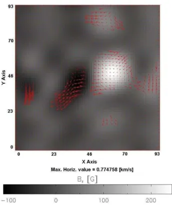
We applied the model to an EUV-BP detected on 19 Jan-uary 2006. To obtain the velocity responsible for the evo-lution of the photospheric magnetic structures associated to the BP we used the local correlation tracking (LCT) tech-nique (November and Simon, 1988). First, the LOS compo-nent of the photospheric magnetic field was filtered using a Fourier filter to select the first eight modes of interest. Then, LCT was applied to the filtered magnetograms separated by a time interval of approximately 30 min, covering the interval between 16:00 UT and 16:30 UT. As a result we obtained a velocity pattern, which is shown in Fig. 1. The formally ob-tained horizontal motion around the positive magnetic field concentration was, however, an effect of the emergence of magnetic flux in that region interpreted by LCT as a horizon-tal velocity pattern (D´emoulin and Berger, 2003). For this reason, we focused the simulation on the horizontal motion derived from the displacement around the negative magnetic field concentration. In the simulation model this motion was approximated by using a combination of vortices of veloc-ity (Fig. 2). The initial three-dimensional magnetic field was obtained from a potential extrapolation of the filtered LOS photospheric magnetogram obtained at 16:00 UT using the algorithm described in Otto et al. (2007).
Fig. 1. Horizontal velocity obtained using LCT technique applied
to the filtered magnetic field in the interval 16:00 UT - 16:30 UT on Jan 19t h2006.
Fig. 2. Horizontal velocity used as boundary condition of the model
to approximate the velocity pattern obtained in Fig.1.
4 Results
The applied photospheric plasma motion gave rise to elec-tric currents just above the region where it was applied, over
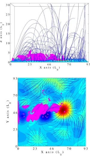
Fig. 3. Lateral view from the negative y-direction (top panel) and
top view (bottom panel) of the isosurfaces of a perpendicular current j⊥=2j0, at t = 1300 s. The isosurfaces of perpendicular current are shown in yellow.
the main polarities of the magnetic field. Figure 4 shows the isosurface of a parallel current jk=2j0, where j0=µB0
0L0 is the value used to normalize the electric current. This current system results from the application of the velocity pattern of Fig. 2 as a boundary condition to the model. This velocity pattern moves the negative polarity region southward, away from the positive polarity. The motion stretches the magnetic flux tubes, increasing their magnetic energy contents. The horizontal motion also gave rise to electric currents perpen-dicular to the magnetic field. Figure 3 shows the isosurface of a perpendicular current j⊥=2j0. The parallel and
per-pendicular currents form just below the solar corona, in the solar atmosphere, and the perpendicular component is less distributed than the parallel component. Note that the cur-rents near the boundary are artifacts of the simulation. The profiles of the current energy
Ej(z) = Z
A
32 J. C. Santos and J. B¨uchner: MHD simulation of electric current formation in the solar atmosphere
Fig. 4. Lateral view from the negative y-direction (top panel) and top view (bottom panel) of the isosurfaces of a parallel cur-rent jk=2j0, at t = 1300 s. The isosurfaces of parallel current are shown in magenta.
are shown in Fig. 5 for the parallel and the perpendicular cur-rents at t = 1300 s. In this profile the current energy start to increase below z = 15 L0, i.e. near and below the transition
region. The energy associated with the parallel current dom-inates over that associated to the perpendicular current.
We also calculated the evolution in time of the total mag-netic energy inside the simulation box
EB = Z V B2 2µ0 dV . (9)
Figure 6 shows the total magnetic energy, in Joules, versus time. It shows that the total magnetic energy increases while the opposite magnetic polarities were moved apart.
5 Conclusions
Our simulation has shown that the horizontal motion of the photospheric plasma and magnetic flux gave rise to electric
Fig. 5. Height profile of the current energy obtained at t = 1300 s.
The height at z = 5 corresponds to the transition region height.
Fig. 6. Total magnetic energy (joules) versus time (τA).
currents mainly in the chromosphere, transition region and lower corona. The currents formed above the region where the motion was applied and above the main concentrations of magnetic field. The component of the electric current par-allel to the magnetic field was stronger and spatially more extended than the component perpendicular to the magnetic field. The latter appeared as kernels of current concentration as shown previously in B¨uchner (2006).
A comparison with TRACE data showed that the area where the current system formed coincides with the area where the EUV-BP appeared (M. Madjarska, private commu-nication). If a temporal sequence of images from trace is an-alyzed one important characteristic is that indeed the bright-ening is always distributed approximately in the same area and the kernels of brightening move inside this area. If the mechanism of heating by DC current dissipation would be efficient, as suggested by B¨uchner and Elkina (2005, 2006),
this current distribution could explain the appearance of the bright point in TRACE data. The fainter extended bright-ening could be associated to the heating caused by the dis-tributed system of currents parallel to the magnetic field, and the moving brighter kernels would be associated to the more efficient dissipation of the kernels of current perpendicular to the magnetic field (B¨uchner and Daughton, 2006).
Acknowledgements. J. C. Santos would like to acknowledge the
International Max-Planck Research School-IMPRS that supported this work by means of a PhD fellowship.
Edited by: H.-J. Fahr
Reviewed by: F. Verheest and another anonymous referee
References
Alfv´en, H.: Granulation, magneto-Hydrodynamic waves and the heating of the solar corona, Mon. Not. Roy. Astron. Soc., 107, 211–219, 1947.
B¨uchner, J.: Locating current sheets in the solar corona, Space Sci. Rev., 122, 149–160, 2006.
B¨uchner, J. and Daughton, W.: Reconnection of Magnetic Fields: Magnetohydrodynamics, Collisionless Theory and Observations, edited by J. Birn and E. R. Priest, Cambridge: Cambridge Uni-versity Press, 144-153, 2007.
B¨uchner, J. and Elkina, N.: Vlasov code simulation of anomalous resistivity, Space Sci. Rev., 121, 237–252, 2005.
B¨uchner, J. and Elkina, N.: Anomalous resistivity of current-driven isothermal plasmas due to phase space structuring, Phys. Plas-mas, 13, 2304–2313, 2006.
B¨uchner, J., Nikutowski, B., and Otto, A.: Magnetic coupling of photosphere and corona: MHD simulation for multi-wavelenght observations, in Multi-Wavelength Investigations of Solar Activ-ity, Proc. IAU Symp., 223, 353–356, 2004.
B¨uchner, J., Nikutowski, B., and Otto, A.: Coronal heating by
tran-sition region reconnection, Proc. SOHO 15 Workshop, Coronal Heating, St. Andrews, Scotland, 6–9 September 2004, ESA SP-575, 2004.
B¨uchner, J., Nikutowski, B., and Otto, A.: Plasma acceleration due to transition region reconnection, Particle acceleration in astro-physical plasmas: Geospace and beyond, edited by D. Gallagher, AGU monograph, Washington, 161–170, 2005.
D´emoulin, P. and Berger, M. A.: Magnetic energy and helicity fluxes at the photospheric level, Solar Physics, 215, 203–215, 2003.
Longcope, D. W.: A model for current sheets and reconnection in x-ray bright points, Astrophys. J., 507, 433–442, 1998.
Madjarska, M. S., Doyle, J. G., Teriaca, L., and Banerjee, D.: An EUV bright point as seen by SUMER, CDS, MDI and EIT on-board SoHO, Astron. Astrophys., 398, 775–784, 2003.
November, L. J. and Simon, G. W.: Precise proper-motion measure-ment of solar granulation, Astrophys. J., 333, 427–442, 1988. Otto, A., B¨uchner, J., and Nikutowski, B.: Force-free magnetic field
extrapolation for MHD boundary conditions in simulations of the solar atmosphere, Astron. Astrophys., 468, 313–321, 2007. Parker, E. N.: Topological dissipation and the small-scale fields in
turbulent gases, Astrophys. J., 174, 499–510, 1972.
Parnell, C. E., Priest, E. R, and Titov, V. S.: A model for x-ray bright points due to unequal cancelling flux sources, Solar Physics, 153, 217–235, 1994.
Priest, E. R., Parnell, C. E., and Martin, S. F.: A converging flux model of an x-ray bright point and an associated canceling mag-netic feature, Astrophys. J., 427, 459–474, 1994.
von Rekowski, B., Parnell, C. E., and Priest, E. R.: Solar coronal heating by magnetic cancellation - II. Disconnected and unequal bipoles, Mon. Not. Roy. Astron. Soc., 369, 43–56, 2006. Roussev, I., Galsgaard, K., and Judge, P. G.: Physical consequences
of the inclusion of anomalous resistivity in the dynamics of 2D magnetic reconnection, Astron. Astrophys., 382, 639–649, 2002. Seehafer, N.: Determination of constant α force-free solar mag-netic fields from magnetograph data, Solar Physics, 58, 215–223, 1978.