Data and Algorithms for Genomic Physical
Mapping
by
Alan P. Kaufman
Submitted to the Operations Research Center
in partial fulfillment of the requirements for the degree of
Master of Science
at the
MASSACHUSETTS INSTITUTE OF TECHNOLOGY
September 1994
(© Massachusetts Institute of Technology 1994. All rights reserved.
Author
... ...
Operations Research Center
July, 1994
/r
Certified
by...-r. v...
/
James B. Orlin
Professor of Operations Research
Thesis Supervisor
Accepted
by..
...
.-.-.-
...
,..-
...
Richard C. Larson
Professor of Electrical Engineering
;ions Research Center
Data and Algorithms for Genomic Physical Mapping
by
Alan P. Kaufman
Submitted to the Operations Research Center on July, 1994, in partial fulfillment of the
requirements for the degree of Master of Science
Abstract
This thesis presents the first independent assessment of two physical mapping projects: the CEPH-Genethon fingerprint mapping effort and the CEPH-Genethon ALU-PCR mapping effort.
The fingerprint data are found to contain numerous errors. Three novel statistics are developed to use these data to determine overlapping pairs of CEPH-Genethon YACs. The best of these statistics is of comparable power to the more sophisticated CEPH-Genethon LOS measures. One novel statistic has proved useful in resolving ambiguous YAC-STS addresses, with concomitant savings in laboratory time and resources.
The ALU-PCR data and their accompanying map construction strategy generate a map with numerous errors. In particular, this strategy treats one-third of the ALU-PCR probes as "wild-card" probes, valid on any chromosome. The CEPH-Genethon strategy applies a single-copy probe mapping algorithm to multiple-copy probes. The resulting map is riddled with spurious connections. An improved map construction strategy is developed using insights from graph theory.
Thesis Supervisor: James B. Orlin Title: Professor of Operations Research
Acknowledgments
I wish to thank Professor Jim Orlin for his support, patience, and advice. I wish to thank my family for their support and encouragement.
Finally, I wish to thank Sara Elisabeth. With her, every day is wonderful, and life is a great party-on-wheels.
Contents
1 Introduction
2 Fingerprint Mapping Literature Review
2.1 Bayes Law and Overlap Detection . . . 2.2 The Yeast Genome ...
2.2.1 Experimental Method . 2.2.2 Pairwise Overlap Detection 2.2.3 Contig Assembly.
2.2.4 Comment ... 2.3 The Worm Genome ...
2.3.1 Experimental Method . 2.3.2 Pairwise Overlap Detection 2.3.3 Contig Assembly.
2.3.4 Comment ...
2.4 The Escherichia Coli Genome . 2.4.1 Experimental Method . 2.4.2 Pairwise Overlap Detection 2.4.3 Contig Assembly ... 2.4.4 Comment ...
2.5 The Human chromosome 16 .... 2.5.1 Experimental Method . . 10 11 12 12
...
12
13 14 15 15 15 ... 1 18 18 18... ... 18
19 20 20 21 21...
...
...
...
...
...
...
...
...
...
...
...
...
...
...
...
...
...
2.5.4 Comment ...
2.5.5 Other Applications of Chromosome 16 Fingerprints
2.6 The Human Genome ...
2.6.1 Experimental Method.
2.6.2 Pairwise Overlap Detection ... 2.6.3 Contig Assembly.
2.6.4 Early Data Problems ... 2.6.5 Comment.
2.7 The Five Projects Compared ... 2.8 The Lander-Waterman Model ...
3 CEPH-Genethon Fingerprints
3.1 Real Data and Simulation . . . 3.2 Data Format ... 3.3 Optical Densities ... 3.4 Band Sizes ... 3.4.1 Problems. 3.4.2 Impact. 3.5 YAC Length ... 3.6 Number of Bands.
3.7 Band Measurement Uncertainty
4 Pairwise Fingerprint Tests
4.1 The Trinomial Test .
4.2 The Match Test ... 4.3 The Entropy Test ... 4.4 The KPN and THE Tests . .
4.5 Evaluating the Tests . . .
4.5.1 Chance Matches.. 4.5.2 Using the Test Bed 4.6 Test Results ...
. . . ...
... 24
. . . ... . . 24 . . . 25 . . . 25... . .26
... . .27
... . .27
... . .28
... . .28
... . .28
33 . . . 33 . . . 34 . . . 35 . . . .35 . . . 35 . . . 38 . . . .. 39 . . . .39 . . . .40 42 43 45 49 52 53 54 56 56...
...
...
...
...
...
...
...
4.7 Uses of Pairwise Overlap Tests ...
4.8 Conclusion...
5 Mapping with ALU-PCR Probes
5.1 Probe Mapping Literature Review ... 5.1.1 Mapping with Single-Copy Probes ... 5.1.2 Mapping with Multiple-Copy Probes ... 5.2 The CEPH-Genethon ALU-PCR Map .
5.2.1 The CEPH-Genethon Datasets ... 5.2.2 The CEPH-Genethon Strategy. ... 5.2.3 Reported Results ...
5.3 ALU-PCR Map Evaluation ...
5.3.1 Problems with the CEPH-Genethon Strategy 5.3.2 Problems with the CEPH-Genethon Map .... 5.4 ALU-PCR Map Remedies ...
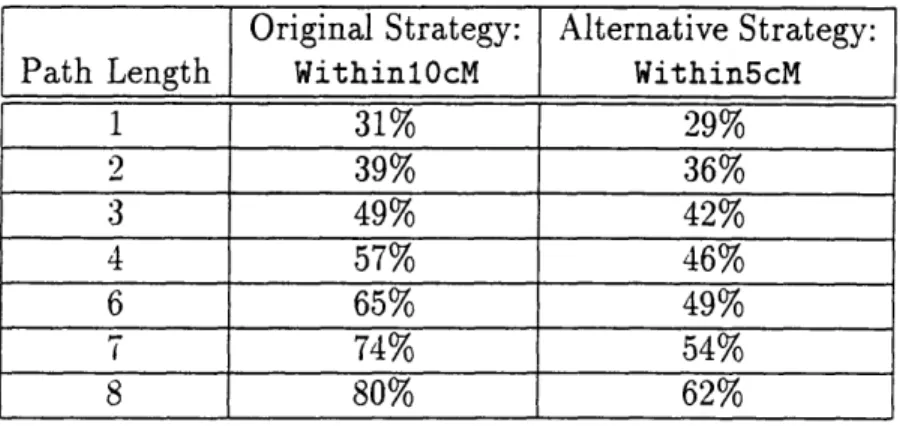
5.4.1 Alternative Strategy: Within5cM.
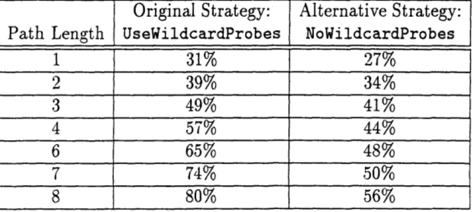
5.4.2 Alternative Strategy: NoWildcardProbes .... 5.4.3 Alternative Strategy: Win5/NoWild.
5.5 Conclusion . ... 6 Conclusion A Glossary B Figures 57 59 60
... ..
60
60 62 63 64 67 69 69 69 71 75 76 77 79 81 82 84 90List of Figures
B-1 Yeast Map Sample (Olson et al. 1986) ... B-2 Worm Map Sample (Coulson et al. 1986) ...
B-3 Bacterium Map Sample (Kohara et al. 1987).
B-4 Chromosome 16 Map Sample (Stallings et al. 1990) . . . B-5 Mapping Project Features ...
B-6 Implied Thetas, Five Projects.
B-7 Original CEPH Data Format ... B-8 Current CEPH Data Format ...
B-9 Optical Intensities of CEPH Fingerprint Bands ... B-10 CEPH Fingerprint Band Size, KPN ...
B-l CEPH Fingerprint Band Size, THE ...
B-12 Fine Histogram of CEPH Fingerprint Band Size ...
B-13 YAC Lengths.
B-14 Number of Band Histograms ... B-15 Number of Band Scatter-plots ...
B-16 Justifying qi = pgainxiYi with Linear Regression ... B-17 Correlation between THE and KPN ...
B-18 Matches by Chance in 10000 Random Pairs ... B-19 False Negative and False Positive Rates, Trinomial Test B-20 False Negative and False Positive Rates, Match Test . . . B-21 False Negative and False Positive Rates, Entropy Test B-22 False Negative and False Positive Rates, KPN Test .... B-23 False Negative and False Positive Rates, THE Test ....
91 91 92 92 93 93 94 95 96 97 98 99 99 ... .. 100 ... ... 101 ... ... 101 ... .. 102 ... .. 102 ... .. 103 ... ... 103 ... .. 104 ... .. 104 ... .. 105
B-24 Efficiency, Trinomial Test ... B-25 Efficiency, Match Test ... B-26 Efficiency, Entropy Test ...
B-27 Efficiency, KPN Test ... B-28 Efficiency, THE Test ...
B-29 Test Efficiencies Compared ...
B-30 Test Efficiencies Compared, Small False Positive Rate B-31 ALU Probe Screening Example ...
B-32 A Spurious Tree ...
B-33 Chromosomes Reached With Short Paths from Probes B-34 Fraction of Connected STS Pairs ...
B-35 Fraction of Truly Connected STS Pairs . . . .
B-36 Fraction of Connected STS Pairs, Scrambled Data . . .
...
105
...
106
...
106
107...
107
...
108
...
108
109 109...
110
...
110
...
111
...
111
B-37 Genome Coverage Using CEPH-Genethon Rules, Real and Scrambled B-38 Genome Coverage Using WithinlOcM and Within5cM . . . .
B-39 Genome Coverage Using Within5cM Real and Scrambled.
B-40 Genome Coverage Using UseWildcardProbes and NoWildcardProbes
B-41 Fraction of Connected STS pairs Using NoWildcardProbes .. . . . B-42 Fraction of Truly Connected STS Pairs Using NoWildcardProbes . .
B-43 Genomic Coverage Using NoWildcardProbes, Real and Scrambled Data
115
B-44 Genomic Coverage Using NoWildcardProbes and Within5cM, Real and
Scrambled Data ... 112 112 113 113 114 114 115
List of Tables
3.1 Mean Band Size ... 36
3.2 Correlation Coefficients, Number of Bands ... 40
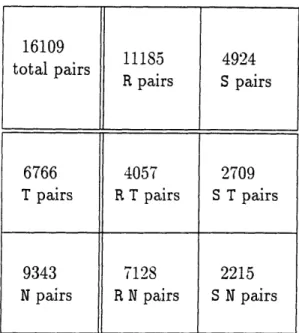
4.1 Breakdown of Test bed clone pairs ... 54
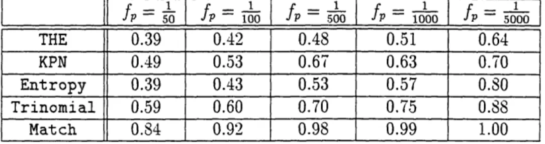
4.2 False Negative Rates ... 57
5.1 Chromosomal Assignments of CEPH-Genethon ALU-PCR Probes . . 67
5.2 Implied Chromosomal Assignments . . . ... 72
5.3 Genomic Coverage ... 77
Chapter 1
Introduction
Physical maps of the human genome order landmarks and DNA fragments along the human chromosomes. Such maps are invaluable tools in the battle against human genetic diseases. Different strategies exist for developing such maps. This thesis examines two strategies: overlap detection via restriction enzyme fingerprints and overlap detection via hybridization probes.
Chapter two reviews the literature on fingerprint mapping. Chapter three ad-dresses the mathematics of fingerprint-based tests for determining pairwise clone overlap. Chapter four applies these tests to real and simulated data and investigates their implications for contig construction.
The last chapter examines probe mapping methods. Chapter five reviews the CEPH-Genethon ALU-PCR mapping project. The chapter highlights problems in the CEPH-Genethon map and proposes some partial remedies.
This thesis focuses on overlap detection, mapping algorithms, and data assess-ment. Except where relevant to the mathematics, detailed explanations of underly-ing biological mechanisms are generally avoided. Some biological terms are defined briefly in Appendix A. Daggerst accompany their first occurrence in the text. The reader may consult the excellent overview of the Human Genome Project [16] or a recent, comprehensive masters thesis [19] for more details.
Chapter 2
Fingerprint Mapping Literature
Review
This chapter reviews recent mapping projects, strategies, analysis methods, and al-gorithms involving restriction enzymet fingerprint patterns.
Before 1986, restriction fragment mapping projects had covered small regions, 50-100 kilobasest in size. The methods of these projects were not suitable for larger
regions.
In 1986, two mapping projects simultaneously attempted a radical new strategy: fingerprinting librariest of randomly created clonest. This method allowed the map-ping of much larger regions, and proved successful for the 15 megabaset genomet of the yeast Saccharomyces and the 80 mb genome of the nematode worm
Caenorhabdi-tis elegans. In 1987, a similar approach mapped the 4.7 mb genome of the bacterium Escherichia Coli. The first mathematical analysis of fingerprint mapping appeared in
1988. In 1990, the strategy was applied to Human Chromosomet 16, 90 mb in length. The most ambitious use of the method occurred in 1992: a massive fingerprinting effort on a random clone library in an attempt to map the entire Human Genome, 3300 mb in length.
Differing in their digestion methods, analysis techniques, and size, these projects
enjoyed varying levels of success. Following a section on Bayesian assessment of
to the success or failure of these projects.
2.1 Bayes Law and Overlap Detection
One may use Bayes Law to write the probability that two clones overlap conditional on observing some data, D, and the prior probability of overlap, poL. To be precise, overlap is a continuous characteristic. Defining a minimal overlap threshold converts this continuous quantity into a binary result. The following basic results consider overlap as a binary characteristic. Continuous overlap models are introduced in Sec-tion 2.6.2.
P( OVERLAPID) = P(DI OVERLAPOL (2.1)
P(D)
This may be written in terms of a likelihood function, L(D).
L(D) = P(DI NO OVERLAP) (2.2
P(DI OVERLAP)
P( OVERLAPID)
(
+
1
POLL(D))
(2.3)
Equation 2.1 or Equation 2.3 represent the correct way to compute a posterior overlap probability from an observation and a prior.
2.2 The Yeast Genome
2.2.1 Experimental Method
In 1986, Olson et al. [43] created a library of 5000 A clones, each containing an insert of yeast DNA. The average insert size was 15 kb, providing 5-fold coverage of the 15 mb yeast genome. Chimerismt, deletionst, or other cloning difficulties were not reported, reflecting the relative stability of the A vector.
generic term "RH" was used to refer to the double digest cleavage sites. EcoRI and HindIII are both 6-cutters. Using the random-base DNA modelt, which crudely models the four bases of DNA as equally probable, a given 6-cutter recognition sitet occurs every 4-6 bases on average. The double digest cuts this distance by half. Thus,
one expects each 15 kb A clone to contain 7.3 RH sites, producing 8.3 RH fragments.
The observed mean was 8.36 fragments.
Gel photographs were projected onto the surface of a digitizing tablet and man-ually traced. The raw images were converted to fragment sizes in basepairs by polynomial interpolation against control bands of known size.
2.2.2 Pairwise Overlap Detection
Pairwise comparisons were made between pairs of fragment size lists. The two lists
corresponded to the fragments of two clones, or of one clone and a partially built
composite map. In the second case, the list corresponding to the partial map was designated the 'reference list", and the list corresponding to the clone was designated the "comparison list." If both lists were single clones, the assignment of "reference" and "comparison" was arbitrary.
The yeast team did not adopt the Bayesian approach described in Section 2.1. Instead, apparent overlap between the pairs of lists was determined using a combina-tion of statistical heuristics. First, each list was scanned independently for intra-list fragment identities. Adjacent bands falling within a thin "identity window" were merged into one. For a list corresponding to a clone, this operation removed doubly traced bands (data entry errors). For a list corresponding to a map, this operation produced a consensus fragment size from its multiple measurements. Next, similar bands between the two lists were paired if they fell within an "error window." Bands were not multiply paired. The width of this error window was expanded linearly with the size of the reference list fragment. This corresponds to a model of fragment measurement error with a standard deviation proportional to fragment length. The proportionality constant was not reported in [43].
rule. This notation is maintained throughout the thesis. Let xa,, xa2,..., an denote
the sizes of the a fragments in the reference list and xb1, xb2, ... , xbn denote the sizes
of the b fragments in the comparison list. Let mal, ma 2,..., man indicate paired
fragments in the reference list: mai = 1 if the reference fragment i matches some fragment from the comparison list, and mai = 0 otherwise. Indicator variables for
the comparison list,
mb,,mb 2,... , mb,,are defined analogously. Let s
= Emai =E mbi denote the number of matched fragments. Let dl, d2, . , ds denote the percent
discrepancies of matched fragments, with mean d = di/s.
The yeast project overlap rule had four components:
Enough matches: s > kl
Not too many mismatches: max(an - s, b - s) < k2
Mutual Overlap Statistic: s2/nanb > k
3
Adjusted Fit: E(di - d)2/s < k4.
Olson et al. considered an overlap significant when it satisfied these conditions with kl = 4 matches, k2 = co mismatches, k3 = 0.60, and k4 = 1%.
2.2.3
Contig Assembly
Connected components in the clone-clone overlap graph provided preliminary, un-ordered contigst. 85% of the clones fell into 680 contigs. The average contig size was 6.2 clones. Simulations indicated that an expected 10 false linkages would be generated by this overlap procedure, implying that an expected 10 of the 680 contigs linked unrelated sets of clones.
Topological constraints imposed by restriction fragment mapping were used to refine the preliminary contigs. Restriction mapst of the contigs were constructed with a greedy algorithm. An initial "seed clone" was selected. The best matching clone in the remainder of the contig was aligned against it, matching RH sites. Additional
were removed from the contig. According to the yeast mapping team, this method removed all incorrect linkages in the preliminary contigs.
Restriction-mapped contigs were oriented and aligned using end clone fragments. The overlap conditions were relaxed so multiple weak relations between end clones could connect contigs.
2.2.4
Comment
The yeast project did not employ the correct Bayesian approach of Section 2.1 and did not justify their ad-hoc overlap test. However, this test was only used to gener-ate preliminary contigs. Creating restriction maps ordered and verified each contig, improving map quality significantly.
According to the yeast mapping team. the final map covered 95% of the genome. Figure B-1 displays a portion of the yeast map.
2.3 The Worm Genome
2.3.1
Experimental Method
In 1986, Coulson et al. [17] amalgamated a heterogeneous library of cosmid and A clones from various Caenorhabditis elegans research labs. The library contained about
8000 clones. The average insert size was 34 kb. This provided 3-fold coverage of the
worm's 80 mb genome. (Additional cosmids, As, and eventually YACSt were later added to the library, bring the total number of clones to over 17000 and the coverage to 18.[53]) It is interesting to note that this article, unlike the article announcing the yeast map [43], did not highlight these essential statistics. The relevant information is buried in the text and in figure captions. A mathematical analysis of fingerprint mapping had yet to be published[34]; thus, the analytical relationship between map quality and genome coverage, genome size, library size, and overlap detection sensi-tivity was unavailable.
tagged and digested again with Sau3Al, a 4-cuttert. The lengths of tagged fragments were measured using electrophoresist. Thus, most measured fragments corresponded
to intervals of DNA flanked by a HindIII site on one side and a Sau3A site on
the other. To be precise, a fragment could have been flanked by two HindIII sites. However, under the random-base DNA model, HindIII-HindIII intervals which lacked a Sau3A site were rare. Using standard results on competing poisson processes[21], the probability that a gap begun at a HindIII site terminated with a HindIII site was
4-+4-4, or less than 0.06. The chance the gap terminated with a Sau3Al site was
over 0.94.
Thus, the number of fragments from a clone (roughly) equals twice the number HindIII sites on the clone. The expected number of fragments is
34 kb x 1 HindIII site 2 frags
46 bp 1 site'
or 16.6 fragment per clone. Coulson et al. reported an average of 23 fragments per clone. This statistically significant discrepancy is consistent with larger inserts (47 kb) or a greater frequency of HindIII sites (1.5 times greater than the random-base rate of 4-6).
After electrophoresis, gel bands were entered manually using a digitizing tablet or semi-manually by digitization with human confirmation. Bands were standardized against control bands of known size, but these measurements were left in mm and not converted to basepairs. Coulson et al. felt
... no useful information is served by [converting from gel measure-ments to bp estimates] because, in our strategy, the lengths of the frag-ments convey no information about the length of the clone. Furthermore, since the gels are denaturing there is no precise correlation between molec-ular size and position (although a given fragment will always run at the same position.)[53]
2.3.2 Pairwise Overlap Detection
The worm project did not adopt the Bayesian methodology of Section 2.1. Instead, they based their overlap calculation on P(DI NO OVERLAP), which they termed
PROBCOINC, for "probability of coincidence." [53]
As equations 2.2 and 2.3 indicate, the absolute size of P(DI NO OVERLAP) is irrelevant. What matters is L(D), the relative likelihood of P(DI NO OVERLAP) to P(DI OVERLAP). L(D) < 1 implies overlap is more likely than nonoverlap, and
L(D) > 1 implies nonoverlap is more likely than overlap. Further, the significance of
a "large" or "small" L(D) value depends on the prior, PoL.
Nonetheless, Coulson et al. used PROBCOINC to determine pairwise clone over-laps. The notation of Section 2.2.2 is maintained. Without loss of generality, let an > b,, so "reference list" refers to the clone with more bands and "comparison list"
to the clone with fewer. Let LGEL denote the length of the sequencing gel, in mm. Let the LTOL denote the tolerance of the sequencing gel: band ai can be matched to band bj if [Xai - Xb I < 2LTOL. This corresponds to fragment measurement error that
does not vary across the gel.
Let p denote chance a band from the comparison list matched a band from the reference list.
p
=
=P(
1)
= - I LGL(2.4)
Using the binomial probability mass function,
B(k, n, p)
= ()pk(l - p)-, (2.5)Coulson et al. defined PROBCOINC to be probability of observing s or more matches:
bn
PROBCOINC = E B(k, bn,p). (2.6)
k=s
Note that this model assumes that bands are independently and identically distributed uniformly across the gels. Also, Equation 2.4 allows the double matching of bands, even though the matching algorithm was not permitted to do so.
2.3.3
Contig Assembly
The worm mapping team used a semi-manual method for contig assembly. Consid-ering pairs of clones with sufficiently small PROBCOINC to be linked, connected components in the clone-clone overlap graph provided preliminary unordered contigs. Humans, assisted by a variety of subroutines which considered local structures in the clone-clone overlap graph, ordered and aligned these preliminary contigs. The sub-routines assembled contigs in a greedy manner, starting with the most probable clone pair overlaps. Unlike the yeast mapping project, which used restriction mapping to exploit the higher discriminating power of many-to-many clone relations, the worm mapping project relied solely upon binary PROBCOINC relations.
2.3.4
Comment
Like the yeast mapping project, the worm project did not employ the correct Bayesian approach of Section 2.1. Unlike the yeast project, the worm project did use a formal model of overlap. By considering only pairwise relations and ignoring band patterns, however, the worm project lost much of the resolution they might have obtained from restriction mapping.
According to Coulson et al., the final map covered 60% of the nematode's genome with 860 contigs, ranging in size from 35 to 350 kb. Figure B-2 displays a portion of the finished map.
2.4 The Escherichia Coli Genome
2.4.1
Experimental Method
In 1987, Kohara et al. [30] created a library of 3400 A clones, each containing an
insert of E. Coli DNA. The average insert size was 15 kb. This library provided 11-fold coverage of the bacterium's 4.7 mb circular, single-chromosomet genome. 1025
The 3400 clones were partially digested with eight separate single digestions with eight different restriction enzymes: BamHI, HindIII, EcoRI, EcoRV, BgII, KpnI, PstI, and PvuII. These enzymes are all 6-cutters, and the random-base DNA model predicts
an average of 3.6 sites for each in a 15 kb clone. A partial digest fragment can begin
at any site, including the ends, and end at any site, including the ends. Rounding 3.6 up to 4, each partial digest produces about ( 2+) = 15 different fragment lengths
under the random-base model.1
Gel images were entered manually using a digitizing tablet. Chimerism was not mentioned, but deletions were indicated in some clones.
2.4.2 Pairwise Overlap Detection
Like the yeast and worm projects. the E. Coli team did not adopt the Bayesian methodology of Section 2.1. Like the yeast project, the E. Coli project did not calculate explicit overlap probabilities within its overlap test.
To determine overlap, the E. Coli team used only the relative order of the eight varieties of restriction sites. Fragment sizes were not involved in this calculation. Instead, the eight partial digests were run side-by-side on the same gel, and their relative order was determined in a manner analogous to the Sanger or the
Maxam-Gilbert method for DNA sequencing[6].
As the E. Coli genome is 4.7 mb, the random-base model predicts an average of 1150 sites for each enzyme, or 9200 restriction sites in total. Thus, the order of these eight restriction sites on the E. Coli chromosome may be considered a 9200 symbol sequence written in an alphabet of eight symbols.
Assuming the eight varieties of restriction cleavage sites occur at random
through-'This is a back-of-the-envelope calculation, for E(f (x)) / f(E(x)). However, the correct value is quite close. As the chance of a restriction site beginning at any given base is low, the number of 6-cutter restriction sites on a 15 kb fragment under the random-base DNA assumption is well-modeled by a poisson random variable with mean 3.6. Numerical evaluation of this expectation,
E((x+2)) = (i2 e2 363
i=O yields 14.7.
out the genome, the probability of observing a particular restriction site k-mer in a given location is 8-k . For example, the chance that the order of the first six restriction
sites on the genome is EcoRI, EcoRI, BgII, HindIII, BamHI, PvuII is 8-6 = 4 x 10- 6.
The expected number of occurrences of this restriction site 6-mer across the genome is 8-6 x 9200 = 0.035. The number of occurrences of this (or any) restriction site 6-mer across the genome is well modeled by a poisson random variable of mean 0.035. Thus, the probabilities of 0, 1, and 2 occurrences of this 6-mer are 0.966, 0.034, and 0.0006, respectively. Conditional on one or more occurrences, the probability of exactly one occurrence is 0.982. The conditional probability of exactly two occurrences is 0.017. In short, any given restriction site 6-mer probably does not occur on the genome (probability 0.966). If a given 6-mer does occur, it probably occurs just once (prob-ability 0.982). Following this logic, the E. Coli mapping project employed a simple test for overlapping clones: two clones overlap if they share six or more consecutive cleavage sites.
2.4.3 Contig Assembly
The E. Coli mapping project used the methods of multi-alignment shotgun sequence assembly ([6], [37], [44]) to order cleavage sites and clones. Once the correct order of sites had been determined, multiple observations of the same band were averaged to estimate inter-restriction site distances on the map.
2.4.4 Comment
The E. Coli mapping project, like the yeast and worm projects, did not employ the Bayesian approach of Section 2.1. The E. Coli multiple-alignment approach to contig construction imposed topological constraints and yielded good contigs. As this approach considers the relationships between multiple clones at once, this strategy more closely resembles the restriction mapping refinement stage in the yeast project than the simple pairwise relations used in the worm project.
with 70 contigs, ranging in size from 20 to 180 kb. Figure B-3 displays a portion on the finished map.
2.5 The Human chromosome 16
2.5.1 Experimental Method
In 1990, Stallings et al. ([52] [54], [5], [58]) created a library of 26000 cosmid clones.
Each contained an insert of human chromosome 16 DNA. The average insert size was 40 kb. The library was probedt with a (GT)n t probe, yielding 3145 (GT)n positive clones. Assuming 40kb clones2, these provided 1.5-fold coverage of the 85 mb chromosome.
The 3145 clones were digested three times: two single digests with the six-cutterst EcoRI and HindIII, and one double EcoRI-HindIII digest. These digests were run out on gels and digitally scanned. Bands were detected by machine and converted to basepairs. The gels were also blotted onto membranes and probed with (GT)n and CotI repetitive sequencer probes. Thus, the following data were known for each band in each digestion of each clone: its length, its (GT)n hybridizationt status (0 or 1), and its CotI hybridization status (0 or 1).
2.5.2 Pairwise Overlap Detection
The chromosome 16 project did employ the Bayesian approach of Section 2.1 to evaluate pairwise clone overlap probabilities. Instead of directly using the data, D, from a pair of clones, Stallings et al. substituted a statistic, S = f(D). This statistic was applied to the three digests separately. Subscripts "E," "H," and "EH" refer to the EcoRI, HindIII, and EcoRI-HindIII digestions, respectively.
2Assuming (GT)n probes are rare and independent of clone-end digestion sites, clones containing
probes will tend to be larger than average clones. Basic random incidence results[21] indicate the expected length of the 3145 clones was E(L)+ aE) = 40 + 0, but the value of was not reported
S =
{SE, SH, SEH} = {f(DE), f(DH), f(DEH)}.A strategic choice of the statistic f would summarize the complexities of a pair of digestions with a single number, and do so with little loss of information regarding overlap or non-overlap of the pair. For this statistic, Stallings et al. selected a digest likelihood ratio.
S = f(D) _ P(DI OVERLAP, simplifying model) P(Di NO OVERLAP, simplifying model)
Equations 2.7 and 2.2 appear similar, but they are not. The digest likelihood ratio of Equation 2.7 is based upon a simplifying model of the digestions. The resulting ,S then plays the role of D in Equation 2.2. The final clone likelihood ratio, L from Equation 2.2, depends on the distribution of S for overlapping clones and the distribution of S for non-overlapping clones.
Stallings et al. adopted a complex statistic for f. This statistic involved a na x nb matrix, C. An element of this matrix, denoted cij, represented the ratio of the probability xa, and Xb, were two measurements of the same fragment to the probability that x,i and Xb were measurements of two different fragments. Thus C contained likelihood ratios for fragments. The "simplifying model" corresponds to the Lander-Waterman model, described in Section 2.8.
(xai +bj ) (sai +b. )2
HGT . HCOT r e 2 2e (ai+bj (
cj =+
(2.8)
This fragment likelihood ratio involved two parts. The first part, the HGT and
HCOT terms, reflected fragment likelihood ratio obtained by considering only the
hybridization status of the two fragments. The remaining terms provided the fragment likelihood ratio obtained by considering the fragment lengths, where i, denoted the
the length measurement reproducibility.
These fragment likelihood ratios were then combined, accounting for all ways to match the na fragments in one clone against the nb fragments in the other:
k=
E
k=1iV,!N
2
!
ii2,- .ik=I 'E
JJ2....Jk--1
= 1(9=1)
no two indices equal no two indices equal
The complexity of Equation 2.9 is equivalent to the computation of a permanent (a determinant with all subtractions replaced by additions[58]). This computation requires exponential time[55]. The chromosome 16 project computed this statistic for each digest for each pair of clones, a total 3 x (12) 2 15 x 106 times. Parallel com-putation, efficient algorithms, and approximations [58] reduced the all-pairs running time to several hours.
Due to the complexity of this statistic, no algebraic probability density function for random vector {SE, SH, SEH} exists. Stallings et al. determined the density function
of {SE, SH, SEH} given overlapping clones and given non-overlapping clones through
massive simulations of model genomes.
2.5.3
Contig Assembly
Contigs construction occurred in the clone-clone overlap graph, where nodes repre-sented clones and arcs reprerepre-sented overlap probabilities above a certain threshold of certainty. Chimerism was not addressed explicitly, though choosing a sufficiently high certainty threshold would remove overlaps between chimeric clone halves.
Without chimerism. Stallings et al. could order clones within contigs. They used interval graph techniques to coalesce contigs by lowering the overlap probability threshold. However, due to the limitations of contig assembly using pairwise over-lap relations and '... the presence of repeated DNA sequences, [map construction] requires human intervention in various stages of constructing an ordered clone map from experimental data."[58]
2.5.4 Comment
After marveling at the complexity of Equations 2.8 and 2.9, one wonders if the finger-print data quality warranted such intricate analysis. Lacking an algebraic probability density function, the behavior of {SE, SH,SEH} may only be understood through simulation. Sensitivity analysis is thus hindered. It is possible this statistic is driven essentially by the number of matching fragments in the two clones. Such simplifica-tions would have been difficult to detect and confirm using simulation.
Stallings et al. report constructing 460 contigs from their 3145 cosmid clones,
covering 54% of chromosome 16. The average contig size was 106 kb. Given the
1.5-fold coverage of the clone library, these are impressive accomplishments. The success of the project hinged upon probing the restriction fragments; this reduced the minimum detectable overlap considerably. (The effect of this reduction is addressed in Section 2.8.) Figure B-4 presents a portion of the finished map.
2.5.5
Other Applications of Chromosome 16 Fingerprints
Fickett and Cinkosky [22] used the Stallings et al. clone-clone overlap probabilities as data for a genetic algorithmt (GA) to determine good ordered contigs. They crit-icized the sequential greedy method used by the yeast and worm projects (Sections 2.2.3 and 2.3.3) the GA outperformed greedy methods on chromosome 16 data. They used three objective functions to evaluate clone permutations. Efficient horizons in this three-dimensional objective space imposed partial orders on proposed solutions. One objective involved the product of successive overlap probabilities; the second involved the estimated degree of overlap; the third involved the lengths of the clones and the chromosome. Fickett and Cinkosky's GA produced better contigs than those produced by the clone-clone overlap graph theoretic approach used initially. In one in-stance, the GA broke a contig generated by the earlier algorithm, and this correctness of this break was confirmed by FISHt mapping individual clones.reported than those obtained by the overlap graph approach. To build restriction maps, Soderlund et al. used a "noisy consecutive ones"3 and heuristic search
tech-niques. They coded their algorithms into an interactive graphical software package named GRAM for computer-assisted restriction mapping. Restriction maps were the focus of these efforts, not not for improving the chromosome 16 clone map.
2.6 The Human Genome
In 1992, Bellanne-Chantelot et al. ([9], [8], [32], [33]) attempted a daring experiment.
CEPH-Genethoni attempted to map the entire 3300 mb human genome using random clone fingerprinting. Previously, the largest region upon which the method had been used was chromosome 16, at 85mb. Two innovations allowed the CEPH-Genethon team to scale up the method forty-fold: YACS offered significantly larger inserts than cosmids, and automated gel reading equipment speeded data entry.
2.6.1 Experimental Method
The CEPH-Genethon team created a library of 22000 YACS containing human DNA. The average insert size was 810 kb, providing 5-fold coverage of the genome. The YACS underwent three single 6-cutter digestions with the restriction enzymes EcoRI, PvuII, and PstI. After electrophoresis, the gels were blotted and hybridized for the Kpn repetitive sequence. Kpn-containing fragments were detected with chemilumi-nescence, scanned, digitized, and standardized against control bands of known size. (The library has since increased to 33000 YACS, of which 25000 have mean insert size of 1 mb. Another repetitive sequence probe has been added, THE. These additional data and their value are discussed in Chapter 3.)
3
A binary matrix has the consecutive ones property if its rows may be permuted so that ones occur consecutively in all columns. The noisy consecutive ones problem seeks to minimize a function of the number of ones that must be changed to zeroes and the number of zeroes that must be changed to one to produce a matrix with the consecutive ones property.
2.6.2 Pairwise Overlap Detection
The CEPH-Genethon team did adopt the Bayesian framework of Section 2.1. Let la
denote the length of the first clone and lb the length of the second. Let 0 denote the length of their common region of overlap. OVERLAP from Equation 2.1 corresponds to 0 > 0, and NO OVERLAP to 0 = 0. The prior on overlap, POL, is supplemented by a prior probability density function on 0, r(0). As all degrees of overlap are a priori equally likely, the non-informative or flat prior was used for Ir(0).
) 1 -POL 0=0
IPOL
< < min(l,lb)min(a,lb)m
Instead of updating a prior for OVERLAP as in Equation 2.1, the CEPH-Genethon team updated a prior for NO OVERLAP. The mathematics are completely analogous, although the CEPH-Genethon likelihood ratio, LOS(D), is the reciprocal of L(D).
P(O = OID) = + 1 - r(0)) LOS(D) (2.10)
LOS(D) -= f>O() P(DO)dO (2.11)
P(DIO = 0)
Similar to the approach of the chromosome 16 project, the CEPH-Genethon team constructed a matrix of matches between all pairs of fragments whose relative dif-ference was below 3 standard deviations. Let Q(k) denote the set of all matchings
between the bands of clone pair that match exactly k bands, leaving na - k bands unmatched on the first clone and nb - k bands unmatched on the second. (This is analogous to the rightmost two sums in Equation 2.9.) Let w denote a particular matching of bands between the clone pair.
min(na ,nb)
P(DIO) = E E P(wl0) P(DIw) (2.12)
surement error of common bands with a Gaussian distribution. The model assumed the standard deviation. oa, grew linearly with the true fragment size, x.
(xz, _x)2 (Xbj _x)2 1
e
L (x 2
fxai lxbj (Xai Xbjx) = 2w(ax)2
Poisson assumptions for restriction sites, probes, and clone ends were used to derive
P(Dw).
The same probes marked bands in the three digests, so the digests were not independent. For computational tractability, the CEPH-Genethon team treated them as independent.
2.6.3 Contig Assembly
Contigs construction occurred in the clone-clone overlap graph, where nodes repre-sented clones and arcs reprerepre-sented overlap probabilities above a certain threshold of certainty. Fine ordering of contigs was not attempted. A handful of CEPH-Genethon contigs were positioned on metaphaset chromosome spreads using FISH.
2.6.4 Early Data Problems
Even in the early stages of the mapping effort, minor difficulties with the CEPH-Genethon fingerprint data were apparent. These problems included numerous chimeric clones in the YAC library (estimated at 40%), artifactual bands (at least one false positive band was found in 10% of the gels), and missing bands (the false negative rate for bands varied between 10% and 70% rate, dependent on optical density).[33] Further, the reported band measurement error, a, was suspiciously low: 0.3% for 1
kb fragments to 1.7% kb for 20 kb fragments. A 1 kb fragment, however, cannot be
measured within 3 bp resolution on an agarose gel; this far exceeds the resolution of the media.[23]
Additionally, only 6 of the 10 contigs hybridized to a single location on the metaphase chromosomes during FISH verification, using pooled inter-ALU PCRt
probes from the contig clones. The remaining four hybridized to two locations, indi-cating chimeric clones had falsely linked noncontiguous regions of the genome.
For one such contig mapping to chromosome 1q244 and 10pll, its 10 constituent
clones were screened individually against metaphase chromosomes using FISH. Three clones mapped to q24. Four mapped to 10pll. One mapped to lq24 and 10pll.
One mapped to lq24, Xpll, and 7q36, and the last mapped to 10pll and Xpll.
2.6.5
Comment
The exact statistics underlying the CEPH-Genethon LOS measure were not pub-lished in the literature, and the CEPH-Genethon procedure for construction was rudimentary.5 These difficulties seem insignificant when compared to issues of data
quality. Section 2.6.4 mentioned problems reported by Chantelot et al. in [8]. These and others are examined in depth in Chapter 3.
According to the CEPH-Genethon interpretation of their data, their physical mapt covered between 85% and 95% of the human genome with over a thousand contigs. According to Genethon, these contigs ranged from 2 to 10 mb in size. CEPH-Genethon did not publish their map.
2.7 The Five Projects Compared
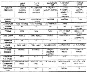
Figure B-5 summarizes salient features of the yeast, worm, bacterium, chromosome 16, and human genome projects.
2.8 The Lander-Waterman Model
Following the yeast, worm, and bacterium projects in the mid 1980s, Lander and Waterman derived simple formulas describing how the clone library and the
finger-4
printing scheme affect the progress of a physical mapping process.[34]
To analyze physical mapping with fingerprints, Lander and Waterman adopted a simplifying model. It considers an idealized fingerprinting method that can detect overlapping clones when they share at least a fraction 0 of their length. It assumes clones are uniformly distributed across the genome. The basic model also assumes 0 is constant across all clones and all clones are of constant length L.
The model uses the following variables: G haploidt genome length in bp,
L clone length in bp.
N number of clones fingerprinted,
a = NIG probability per base of starting a new clone, T minimum detectable overlap length in bp,
c = LN/G redundancy of library coverage,
0 = T/L , and = 1 -0.
Connected components in the clone-clone overlap graph are called apparent islandst. Islands with two or more clones are contigs.
Moving along the genome base by base, a clone begins with probability a. If no other clone begins in the next L - T bases, this clone will be the last in its island. The probability this base starts a clone that ends an island is thus c(1 - a)L- T. This
can be written as a(1 - N/G)(G/N)c , which well-approximated by ae- co for small
NiV/G. As there are the same number of clones that end islands as there are islands, it follows the expected islands is Gae-U = Ne- ([34], Proposition 1.1.)
A similar argument shows the number of clones in an island is geometric with mean ecU. The probability an island contains exactly j clones is (1 -e-c)i-le - c . Thus, the expected number of islands containing j clones is N(1- e-)j-le -c (Prop.
1.2) and expected number of contigs is Ne-c" - Ne- 2c (Prop. 1.2.1.) Lander and
and the expected length of an island, L[((eC" - 1)/c) + (1 - a)] (Prop. 1.4.) By setting 0 = 0, any common DNA suffices for clone-clone overlap, and these results apply to undetected overlap (Prop. 1.5.) With minor modifications, the model can accommodate L and 0 varying across clones (Prop. 2.)
This model allowed biologists to predict the quality of the physical map a set of experiments could be expected to generate-before conducting any experiments.
Given the cost and magnitude of mapping projects, the importance of this model for strategic planning is large. Planning and progress assessment are the conventional, forward uses of this model.
Lander and Waterman note that the decreasing 0 from 0.50 to 0.25 greatly speeds the progress of a mapping project, while decreasing 0 from 0.25 to the theoretical limit of 0 provides relatively less improvement. They suggest 0 values between 0.15
and 0.20 as sensible goals.
How efficient were these five projects in detecting overlap? The Lander-Waterman model has a less conventional, backward use: it allows one to calculate an implied 0 from reported coverage and contig measures. These different performance measures are functions of 0. Solving for 0 is straight-forward.
If x denotes the number of islands,
=
1
+ ln(x/Nc)c
If x denotes the number of isolated clones,
0
1 + ln(x/N)
9=1+
2cIf x denotes the mean island size,
ln(x)
If x denotes the number of contigs, then 0 solves
x = Neh--( 1 ) cu Ne- 2 (1- ) c
This formula can have multiple roots in the unit interval; selecting the root closest to the value of 0 produced by the other performance measures removes this ambiguity.
Figures B-5 and B-6 present 0 values implied by these four performance measures for the five projects. The bacterium project achieved the lowest 0, approximately 0.2. The worm project achieved a 0 of about 0.5; chromosome 16 was slightly higher. The chromosome 16 project produced far more contigs than expected, given the project's reported contig size and number of number of islands. Cloning biases or probe clustering might explain this anomaly. The yeast project achieved a 0 between 0.6 and 0.7, an impressive feat considering its early date. The CEPH-Genethon
project, however, performed poorly, with a 0 value above 0.95.
The efficiency of the E. Coli project and the inefficiency of the CEPH-Genethon projects at detecting overlap reflect their respective strategies for overlap detection. The bacterium project demonstrated the power of shotgun-sequencing analysis tech-niques following partial digestions with multiple restriction enzymest.
It is tempting to consider the map CEPH-Genethon might have obtained with such a strategy and a 0 , 0.2. The E. Coli strategy, however, would not scale up to YAC-sized inserts. Assume 200 clearly resolved bands represents an upper bound on the resolution of current gels. This limits the number of restriction sites per clone to
19+2
about 19: a partial digestion of 19 sites produces about ( 2 ) = 210 fragments. Under
the random-base model, restriction enzymes with 13 bp recognition sites are required to obtain so few restriction sites per megabase clone (109/412.82 - 19). Restriction
enzymes with such long recognition sites are rare, and it is likely that random-base model would not be a realistic representation of their occurrence along genome.
To map the human genome, CEPH-Genethon needed clones with large inserts. As the inserts were large and the resolution of gels was limited, CEPH-Genethon needed probes to select only certain bands from complete digestionst. Because of
these constraints, CEPH-Genethon could not have used the E. Coli approach. The following chapter examines the quality of the CEPH-Genethon data.
Chapter 3
CEPH-Genethon Fingerprints
This chapter reviews the CEPH-Genethon fingerprint data in preparation for sub-sequent evaluation of pairwise overlap tests. The original Kpn-probed data doubled with the addition of a second probe, THE, in 1991. Additional clones were added to the megabase library, bringing the total to 33000 YACs. The fingerprint dataset has since stabilized; no additional experiments are planned. More recently, a dataset
with YAC sizes was also released.[48]
3.1 Real Data and Simulation
Simulation provides a powerful technique to investigate the performance of a finger-print mapping effort. Simulation can encompass any level of detail, providing greater realism than simplified analytic models (cf. [34]). Simulation is also useful when evaluating or tuning pairwise clone overlap tests, for the "right" answer is known.
A fingerprint simulator for pairwise clone overlap test evaluation would include the following: a model of clone lengths and chimeric clones; a model of clone overlap; a model of restriction site spacing; a model of probe spacing (equivalently, the number of bands per clone); a model of band measurement error; and models of false positive and false negative bands.
For example, Datta assumed constant length non-chimeric clones, overlap lengths uniformly distributed across clone lengths, the number of bands and the size of bands
drawn from empirical distributions matching the real data, Gaussian band measure-ment error, and Bernoulli-generated false negatives [19].
Simulation has a disadvantage: a simulator can be inaccurate. Datta found pair-wise overlap statistics that performed admirably on simulated clone pairs performed less impressively on real data [19]. Clearly, his simulation differed from the real data in some unknown but substantive way. Datta's assumptions of non-chimeric and constant length clones are likely candidates, as is his assumption that THE and Kpn probes follow independent poisson processes. In reality. 40% of the clones are chimeric ([8]); clone lengths vary (Section 3.5); the two types of probes are correlated (Section 3.6); the genome consists of "probe-rich" and "probe-poor" regions ([28]); cluster or spread processes ([36]) might better describe probe locations.
This thesis eschews simulation to avoid such difficulties. The interested reader should consult Datta for a comprehensive simulation study paralleling this thesis
[19].
3.2 Data Format
Figure B-7 presents a sample of the original CEPH-Genethon data format. Each
clone has a seven line block of data. Line one identifies the YAC. Lines three, five
and seven indicate the results of the EcoRI, PstI, and PvuII digestions, respectively. For each digestion, an integer indicates the size of a band in base pairs and is followed by a decimal number indicating the optical intensity of the band'. Electrophoresis sorted the bands by size.
The newer dataset differs from the earlier one in two ways. First, the three digestions appear twice, once for each probe. Second, optical density data are not included. Figure B-8 presents a sample of these data.
1The raw gel images were scanned, digitized, and standardized to generate these sizes. The processed band sizes and their intensities were the only data made publicly available.
3.3 Optical Densities
Figure B-9 provides a histogram of band intensity from the earlier data. The mean intensity is 0.30; the median is 0.196; the distribution has a heavy right tail. CEPH-Genethon reported that band reproducibility varied with optical intensity, with a 50% reproducibility rate for bands with optical density below 0.05.[33] 14% of observed bands had densities below this threshold.
There are two possible interpretations of these low reproducibility bands. The first interpretation declares these bands to be weak readings of true bands: false negatives. From the .50% reproducibility rate, roughly each detected weak band has a corresponding undetected band. Assuming every weak band has an undetected pair. this suggests a false negative rate of about 14% 12%. The second interpretation declares these bands to be spurious readings of nonexistent bands:
false positives. In this case, at least 14% of the bands are false.
Such error estimates are informative, for optical intensity data were dropped from the newer release.2 No threshold was imposed; even bands measured at optical inten-sity "0" in the earlier data appear in the newer dataset. Without inteninten-sity data, all bands in the newer data release appear equal, hiding a possible 12-14% false negative or false positive rate.
3.4
Band Sizes
3.4.1 Problems
Under the random-base DNA model, occurrences of a 6-cutter recognition site are well-modeled by a Bernoulli process. The distances between successive recognition sites follow a geometric distribution with mean 46. The placement of probes3 may
2Optical intensity measurements for Kpn bands are available from the earlier dataset. Intensities
for THE bands are not available. CEPH-Genethon ignored intensity data altogether in their analysis;
this thesis does likewise. 3
For all fingerprint chapters in this thesis, "probes" refers to the repetitivet elements Kpn and THE.
If EcoRI PstI PvuII
THE 6755 5549 6760
Kpn 7094 7691 7919
Table 3.1: Mean Band Size
be modeled with another independent Bernoulli process with a much slower rate. (The probes were purposely sparse compared to 6-cutter restriction sites, for CEPH-Genethon used rare probes to obtain a resolvable number of bands after digestion.) With these two modeling assumptions, probes may be considered "random-incidence arrivals" [21] into restriction site gaps. The size of probe-containing inter-restriction gaps follows a second order Pascal distribution with mean 2 x 46 = 8192. This discrete distribution is well-approximated by its continuous counterpart, the second order Erlang.
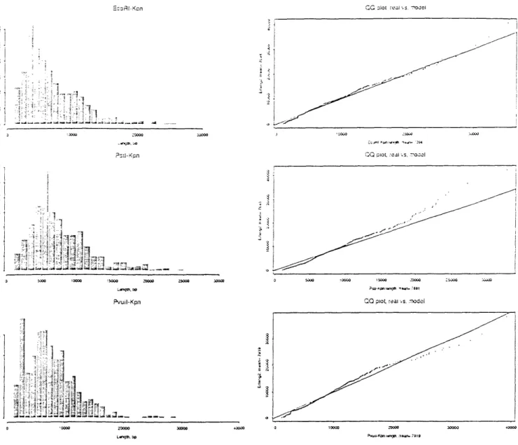
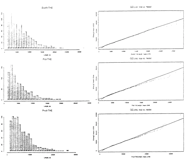
Table 3.4.1 indicates mean band size for all three digests and both probes. That all these means fall below the random-base model prediction of 8192 is not noteworthy; DNA sequence is not Markovian. The order of these means is interesting, however. For THE, PstI had the smallest mean gap, followed by EcoRI and PvuII in an effective tie. For Kpn, the order of increasing means was EcoRI, PstI, PvuII. These rankings are not in agreement, indicating some unknown correlation between probe sites and restriction enzyme recognition sites.
Figures B-10 and B-11 present histograms and QQ-plots of band length for all six probe-digest combinations based on a random sample of 5000 bands. The QQ-plots compare the empirical distributions to second order Erlangs with matched mean. The roughly linear QQ-plots indicate the two distributions are similar. However, both informal inspection of the histograms and formal testing using the X2 statistic
[191 indicate these distributions are not Erlang.
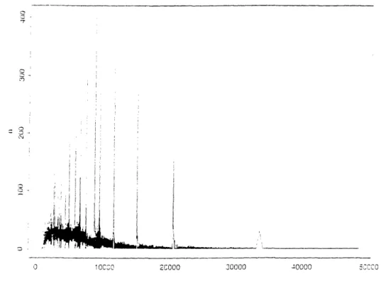
The coarse binning of these histogram hides data anomalies[47]. Figure B-12 presents a detailed histogram of band sizes.4 The x axis of the histogram corresponds
to band size in increments of one basepair, the given data resolution. The y axis corresponds to the number of occurrences of that band size in a random sample of 23% of the data. The figure is a line plot, with straight lines connecting adjacent nonzero counts.
One sees the quasi-Erlang structure of the length distribution as the thick black band that rises until x ~ 8000 and then slowly falls. The thickness of the band corresponds to the range of the counts, an indication of variance. The bottom of the thick black band remains essentially above the x axis until x _ 9000.5
This expected quasi-Erlang structure is punctuated by a series of unexpected large spikes. Small intervals with few observations flank each spike. These nearly empty-gaps are indicated by black lines reaching down to the x axis for the smaller bands. and by empty triangles beneath the larger bands. This gap-spike-gap phenomenon occurs in the same locations across all probe-digest combinations. A systematic error in the gel digitizing hardware or software is the likely explanation. The height of the spikes roughly accounts for the gaps of "missing" probability. Inter-spike spacing seems to increase exponentially with band size, suggesting an error mechanism that occurred at constant intervals along the gel. One might postulate an irregularity in a gear mechanism that drove the digitizing head across the gel films; perhaps a slight velocity hiccup on each revolution collapsed a rectangular region of the image onto a narrow bar.
Other minor anomalies afflict the length data. The dataset contains a handful of extremely long bands. The longest is 283548 bp. The genome is unlikely to contain such a large gap between 6-cutter restriction sites. The YACs average 0.8 mb in length and contain on average less than 16 probes; extrapolating this rate for the whole genome produces an overestimate of 3300 x 16/0.8 = 66000 probes and thus 66000 probe-containing inter-restriction site gaps. Employing a second order Erlang
5If xi denotes the number occurrences of a band of size i in a sample of N bands, the joint distribution of {Xl, x,... 2 , X50000} is multinomial with parameters from the second order Pascal:
pi = (i - 1)(4-6)2(1 _4-6) i-2. The marginal distribution of xi is binomial. A 95% confidence interval for xi is Npi - 2/Npi(1 - Pi). For N z 250000, the bottom of this confidence interval hits zero near i 9000.
with mean 6725 for the band size distribution6, the probability that the genome
contains a gap of size 283548 or larger is approximately
66000 6725-2xe-/ 6 25dx, 83548
which is less than 10-11. Therefore, from mathematical considerations alone, the 283548 band is highly likely to be spurious, as are another six bands longer than 250000. The optimist finds a handful of errors among 1452000 band observations encouraging. The pessimist wonders why such blatant errors were not detected and fixed, and if these errors suggest the presence of additional, undetected problems.
3.4.2 Impact
The band length distribution suffers two main problems: dramatic probability spikes and a handful of observations on the distant right tail. The remainder of the data appear reasonable.
If one assumes the probability spikes collapsed a wider observation region onto a narrow one, this anomaly only serves to reduce the resolving power of the gel over a small set of disjoint regions. As the observations that fell into these regions comprise less than 1% of the total observations, this anomaly should have little effect. If one instead assumes the spikes represent induced false positives at specific spots, this anomaly causes pairs of clones to have an extra few matching bands. As the various pairwise overlap tests are tuned to obtain selected false positive and false negative rates (Chapter 4), this should have little effect. Likewise, the excessively large bands quite rare. As no such band occurs in two clones, such bands are never matched in a pairwise clone overlap test, and thus have little effect.
The impact of these anomalies upon the pairwise overlap tests is expected to be slight. Nonetheless, such problems do erode one's confidence in the quality of these
3.5
YAC Length
Recent CEPH-Genethon data releases have included data on YAC lengths. Figure B-13 presents a histogram of lengths for the fingerprinted YACS7. The histogram
indicates YAC length is highly variable. The mean YAC length is 910 kb, slightly longer than the earlier estimate of 810 kb by Chantelot et al.[8] A uniform distribution between 100 kb and 1750 kb provides a very crude approximation of this distribution.
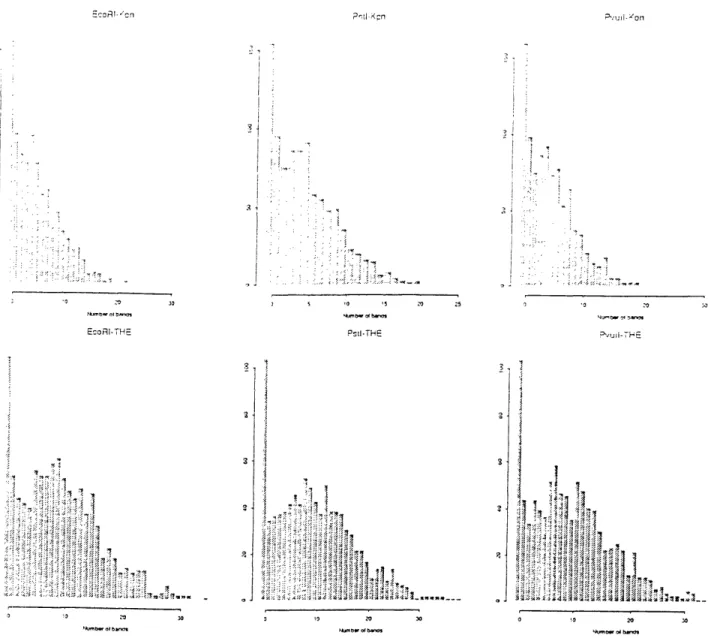
3.6 Number of Bands
Figure B-14 presents histograms of the observed number of bands per YAC.
The number of bands per YAC is not poisson. This is expected, as the clones are of variable length8. The observed probability spikes at zero bands suggest a switching process: with probability p, the YAC has no bands, and with probability 1 - p, the YAC has a poisson number of bands with a mean proportional to its length. YACS with no bands may have come from regions of the genome lacking THE and Kpn repetitive elements or they may represent complete hybridization failure.
Figure B-15 displays the correlation between the numbers of various bands using a scatter-plot matrix. The 3x3 upper left submatrix gives plots of Kpn bands for the three digests. The points are roughly linear and indicate a high positive correlation. This is expected, as each probe should produce one band in each of the three digests. A similar pattern holds for the THE plots in the lower right 3x3 submatrix.
The lower left 3x3 submatrix plots the three digests for Kpn bands against the three digests for THE bands. The points form a diffuse cloud, but a linear
correla-7YACS from plates 628-989 were fingerprinted. Some of these are megabase YACS; the
CEPH-Genethon megabase library consists of plates 713-996 and plates 2000+.
8
If clone lengths were uniformly distributed between 100 kb and 1750 kb and probes followed a poisson process with rate A probes per kb, the probability mass function for the k, the number of bands on an arbitrary YAC, would take the following form:
1
Xf=.75
(Al))e-~,lPK(k) =75 01=175 (Al)ke Aldl.
Except for the spikes at zero bands observed in the real data, this probability mass function with
EcoRI Kpn PstI Kpn PvuII Kpn EcoRI THE PstI THE PvuII THE EcoRI Kpn 1 PstI Kpn 0.93 1 PvuII Kpn 0.94 0.93 1 . EcoRI THE 0.62 0.62 0.62 1 PstI THE 0.62 0.63 0.62 0.94 1 PvuII THE 0.63 0.62 0.63 0.94 0.95 1
Table 3.2: Correlation Coefficients, Number of Bands
tion is still seen. Table 3.6 provides all pairs of correlation coefficients between these counts. The THE-Kpn correlation coefficients exceed 0.6, indicating these two repet-itive elements frequently occur together on the genome. This has two implications. The first is that doubling the data by adding the THE probe did not produce as much additional coverage as might have been obtained with an independent or, better yet, negatively correlated probe. The second implication is that the regions of the genome covered by Kpn-base contigs in 1992 should have stronger overlap results from the additional THE probes in 1993.
3.7 Band Measurement Uncertainty
As mentioned in Section 2.6.4, CEPH-Genethon reported a dubiously low standard deviation for band measurement error: 0.3% for 1 kb fragments to 1.7% kb for 20 kb fragments.
To estimate this rate de novo from the data, a small number of plates in the YAC library with highly similar fingerprints in adjacent wells were identified.9 Plate contamination is the most likely explanation of this phenomenon. This provides repeated measurements of (what is highly likely to be) the same band. The standard deviation, a, was observed to vary slowly with band length, x. Point estimates of
curve was fit to these estimates using least squares regression (R2 > 0.95):
o(x) = 41.9 - 0.0005x + 2.7 x 10-7x2. (3.1)
The details of this estimation are provided by Datta[19]. This thesis employs Equation 3.1 to model band measurement error.