HAL Id: hal-01126612
https://hal.archives-ouvertes.fr/hal-01126612
Submitted on 6 Mar 2015
HAL is a multi-disciplinary open access
archive for the deposit and dissemination of
sci-entific research documents, whether they are
pub-lished or not. The documents may come from
teaching and research institutions in France or
abroad, or from public or private research centers.
L’archive ouverte pluridisciplinaire HAL, est
destinée au dépôt et à la diffusion de documents
scientifiques de niveau recherche, publiés ou non,
émanant des établissements d’enseignement et de
recherche français ou étrangers, des laboratoires
publics ou privés.
Influence of the mass distribution on the magnetic field
topology in spherical, anelastic dynamo simulations
Raphaël Raynaud, Ludovic Petitdemange, Emmanuel Dormy
To cite this version:
Raphaël Raynaud, Ludovic Petitdemange, Emmanuel Dormy. Influence of the mass distribution on
the magnetic field topology in spherical, anelastic dynamo simulations. Journées de la SF2A, Jun
2014, Paris, France. 2014. �hal-01126612�
INFLUENCE OF THE MASS DISTRIBUTION ON THE MAGNETIC FIELD TOPOLOGY IN
SPHERICAL, ANELASTIC DYNAMO SIMULATIONS
R. Raynaud
1, L. Petitdemange
1and E. Dormy
2Abstract. Numerical modelling of convection driven dynamos in the Boussinesq approximation revealed fundamental characteristics of the dynamo-generated magnetic fields. However, Boussinesq models are not adequate for describing convection in stratified systems, and thus the validity of these previous results remains to be assessed for gas giants and stars. To that end, we carried out a systematic parameter study of spherical dynamo models in the so-called anelastic approximation, which allows for a reference density profile while filtering out sound waves for faster numerical integra-tion. We show that the dichotomy of dipolar and multipolar dynamos identified in Boussinesq simulations is still present in anelastic models, and dipolar dynamos require that the typical length scale of convection is an order of magnitude larger than the Rossby radius. However, the established distinction between dipolar and multipolar dynamos tends to be less clear than it was in Boussinesq studies, since we found a large number of models with a considerable equatorial dipole contribution together with an intermediate overall dipole field strength. This tendency can be found in very weakly stratified models, but it was not reported for previous Boussinesq models assuming a homogeneous mass distribution. In contrast, anelastic models usually assume a central mass distribution, which leads to a gravity profile proportional to 1/r2. Actually, we show that this choice can result in changes in the magnetic field topology that are mainly due to the
concentration of convective cells close to the inner sphere.
Keywords: dynamo, magnetohydrodynamics, magnetic fields, stars: magnetic field
1 Introduction
Dynamo action, i.e. the self-amplification of a magnetic field by the flow of an electrically conducting fluid, is considered to be the main mechanism for generating of magnetic fields in the universe for a variety of systems, including planets, stars, and galaxies. Because of the difficulty simulating turbulent fluid motions, one must resort to some approximations to model the fluid flow, whose convective motions are assumed to be driven by the temperature difference between a hot inner core and a cooler outer surface. A strong simplification can be achieved when applying the Boussinesq approximation, which performs well in so far as variations in pressure scarcely affect the density of the fluid. However, this approximation will not be adequate for describing convection in highly stratified systems, such as stars or gas giants. A common approach to overcoming this difficulty is then to use the anelastic approximation, which allows for a reference density profile while filtering out sound waves for faster numerical integration. This approximation was first developed to study atmospheric convection (Ogura & Phillips 1962; Gough 1969). It has then been used to model convection in the Earth core or in stars and is found in the literature under slightly different formulations (Gilman & Glatzmaier 1981; Braginsky & Roberts 1995; Lantz & Fan 1999; Anufriev et al. 2005; Berkoff et al. 2010; Jones et al. 2011; Alboussi`ere & Ricard 2013). Nevertheless, the starting point in the anelastic approximation is always to consider convection as a perturbation of a stratified reference state that is assumed to be close to adiabatic.
Observations of low mass stars have revealed very different magnetic field topologies from small scale fields to large scale dipolar fields (Donati & Landstreet 2009; Morin et al. 2010), and highlight possible correlations between differential rotation and magnetic field topologies (Reinhold et al. 2013). Boussinesq models partly reproduce this diversity (Busse & Simitev 2006; Sasaki et al. 2011; Schrinner et al. 2012). For anelastic models, not only previously proposed scaling laws (Christensen & Aubert 2006), but also the dichotomy between dipolar and “non-dipolar” (or multipolar) dynamos seems to hold (Gastine et al. 2012; Yadav et al. 2013; Schrinner et al. 2014). These are characterized by different magnetic field
1LERMA, Observatoire de Paris, PSL Research University, CNRS, UMR 8112, F-75014, Paris, France 2IPGP, CNRS UMR 7154, 75005 Paris, France
c
274 SF2A 2014
(a) Boussinesq models (Schrinner et al. 2012). (b) Anelastic models (Schrinner et al. 2014).
Fig. 1. fdipversus Ro`. Filled symbols stand for dipolar, open symbols for multipolar dynamos. A cross inscribed in some open symbols
means that the field of these models exhibits a strong equatorial dipole component. In figure (a), the symbol shape indicates different types of mechanical boundary conditions: circles mean no-slip conditions at both boundaries, triangles are models with a rigid inner and a stress-free outer boundary, and squares stand for models with stress-free conditions at both boundaries. In figure (b), the symbol shape indicates the number of density scale heights: N%= 0.5: circle; N%= 1: upward triangle; N% = 1.5: downward triangle; N%= 2:
diamond; N%= 2.5: square; N%= 3, 3.5, 4: star.
configurations: dipolar dynamos are dominated by a strong axial dipole component, whereas multipolar dynamos usually present a more complex geometry with higher spatial and temporal variability. However, as we can see in Fig. 1, this distinction is somewhat less clear for anelastic models, due to the presence of multipolar models with a high equatorial dipole contribution which induces an intermediate dipole field strength.
Raynaud et al. (2014) aim to clarify the reasons likely for the emergence of an equatorial dipole contribution when measuring the dipole field strength at the surface of numerical models. Since our approach closely follows previous methodology for studying the link with Boussinesq results, we decided to focus in more detail on one important change that comes with the anelastic approximation, assuming that all mass is concentrated inside the inner sphere to determine the gravity profile. In contrast, as proposed by the Boussinesq dynamo benchmark Christensen et al. (2001), it was common for geodynamo studies to assume that the density is homogeneously distributed. This leads to different gravity profiles, the first being proportional to 1/r2, whereas the second is proportional to r. We show that the choice of the gravity profile may have strong consequences on the dynamo-generated field topology.
2 Set up
We rely on the LBR-formulation of the anelastic approximation, named after Lantz & Fan (1999) and Braginsky & Roberts (1995), as it is used in the dynamo benchmarks proposed by Jones et al. (2011). A detailed presentation of the equations can be found in Schrinner et al. (2014). We consider a spherical shell of width d and aspect ratio χ= ri/ro, rotating about the z axis at angular velocityΩ and filled with a perfect, electrically conducting gas with kinematic viscosity ν, thermal diffusivity κ, specific heat cp, and magnetic diffusivity η (all assumed to be constant). In contrast to the usual Boussinesq framework, convection is driven by an imposed entropy difference ∆s between the inner and the outer boundaries, and the gravity is given by g = −GMˆr/r2where G is the gravitational constant and M the central mass, assuming that the bulk of the mass is concentrated inside the inner sphere. We impose stress free boundary conditions for the velocity field at both the inner and the outer sphere, the magnetic field matches a potential field inside and outside the fluid shell, and the entropy is fixed at the inner and outer boundaries.
The system is control by seven parameters, namely the Rayleigh number Ra= GMd∆s/(νκcp), the Ekman number E= ν/(Ωd2), the Prandtl number Pr= ν/κ, and the magnetic Prandtl number Pm = ν/η, together with the aspect ratio χ, the polytropic index n, and the number of density scale heights N% = ln (%i/%o) that define the reference state. Raynaud et al. (2014) restrict the investigation of the parameter space keeping E= 10−4, Pr = 1, χ = 0.35, and n = 2 for all simulations. Furthermore, to differentiate the effects related to the change in gravity profile from those related to the
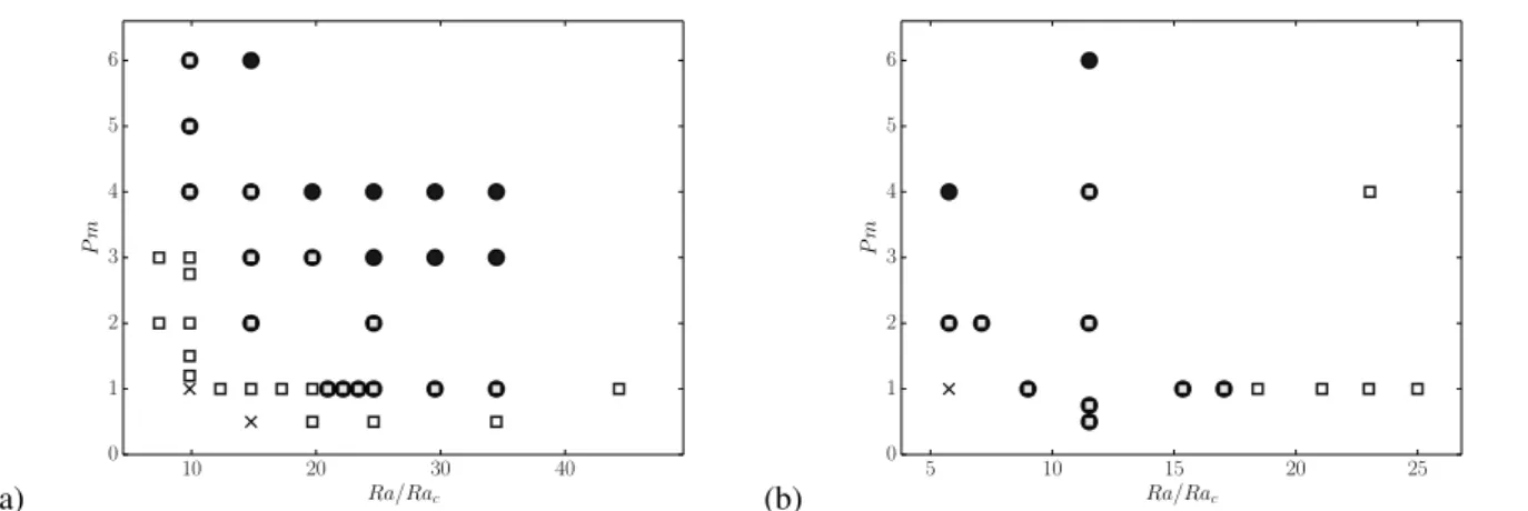
(a) 10 20 30 40 Ra/Rac 0 1 2 3 4 5 6 P m (b) 5 10 15 20 25 Ra/Rac 0 1 2 3 4 5 6 P m
Fig. 2. Dipolar (black circles) and multipolar (white squares) dynamos as a function of Ra/Racand Pm, for a central mass (a) and a
uniform mass distribution (b). Crosses indicate the absence of a self-sustained dynamo.
anelastic approximation, we decided to perform low N% simulations so that we can assume that stratification no longer influences the dynamo process. In practice, we choose N%= 0.1, and the simulations are thus very close to the Boussinesq limit.
A measure of the velocity field amplitude is given by the Rossby number Ro= √2EkE/Pm, where Ekis the kinetic energy density. To distinguish between dipolar and multipolar dynamo regimes, we know from Boussinesq results that it is useful to measure the balance between inertia and Coriolis force, which can be approximated in terms of a local Rossby number Ro` = Roc`c/π, which depends on the characteristic length scale of the flow rather than on the shell thickness (Christensen & Aubert 2006; Olson & Christensen 2006; Schrinner et al. 2012). The dipolarity of the magnetic field is characterized by the relative dipole field strength, fdip, originally defined as the time-average ratio on the outer shell boundary Soof the dipole field strength to the total field strength. We also define a relative axial dipole field strength fdipax by filtering out non-axisymmetric contributions.
3 Results
Figure 2(a) shows the regime diagram we obtained, as a function of the Rayleigh and magnetic Prandtl numbers. For Pm = 1, the transition from the dipolar to the multipolar branch can be triggered by an increase in Ra. In that case, the transition is due to the increasing role of inertia (corresponding to Ro` ∼ 0.1 in Fig. 3). Alternatively, the transition from multipolar to dipolar dynamo can be triggered by increasing Pm. Then, the multipolar branch is lost when the saturated amplitude of the mean zonal flow becomes too small to prevent the growth of the dipolar solution (see Schrinner et al. 2012). It is worth noting that the two branches overlap for a restricted parameter range for which dipolar and multipolar dynamos may coexist. In that case, the observed solution strongly depends on the initial magnetic field, so we tested both weak and strong field initial conditions for all our models to delimit the extent of the bi-stable zone with greater accuracy. Actually, multipolar dynamos are favoured by the stronger zonal wind that may develop with stress-free boundary conditions, allowing for this hysteretic transition. Finally, we see that the dynamo threshold is lower for multipolar models, which allows the multipolar branch to extend below the dipolar branch at low Rayleigh and magnetic Prandtl numbers. We see in Fig. 2(b) that this is different from Boussinesq models with a uniform mass distribution (after Schrinner et al. 2012).
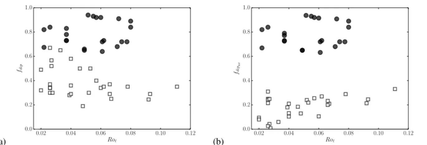
Figure 3(a) shows that the tendency highlighted in Fig. 1(b) already exits at low N%, and thus cannot be accounted for only in terms of anelastic effects. When the equatorial dipole component is removed to compute fdipax, we recover a more abrupt transition, as we can see in Fig. 3(b): dipolar dynamos are left unchanged, whereas multipolar dynamos of intermediate dipolarity are no longer observed, which confirms that the increase in fdip is due to a significant equatorial dipole component. Moreover, we show in Raynaud et al. (2014) that these equatorial dipoles are preferably localized close to the dynamo threshold of the multipolar branch, at low Rayleigh and magnetic Prandtl numbers.
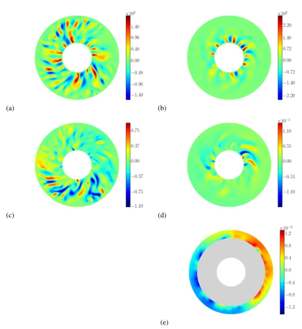
Then, the only significant parameter that is changed between Fig. 1(a) and Fig. 3(a) is the choice of the gravity profile, and this is sufficient to explain the emergence of the equatorial mode. Indeed, with a central mass distribution, convection cells now form and stay closer to the inner sphere, as we can see in Fig. 4(a,b) that shows equatorial cuts of the radial component of the velocity and magnetic fields, for both gravity profiles. This strong difference in the flow reflects on the
276 SF2A 2014 (a) 0.02 0.04 0.06 0.08 0.10 0.12 Ro` 0.0 0.2 0.4 0.6 0.8 1.0 fdip (b) 0.02 0.04 0.06 0.08 0.10 0.12 Ro` 0.0 0.2 0.4 0.6 0.8 1.0 fdip ax
Fig. 3. (a): fdipversus Ro`. (b): fdipaxversus Ro`. The meaning of the symbol shapes is defined in the caption of Fig. 2.
localization of the active dynamo regions (see Fig. 4 (c,d)). With a gravity profile proportional to 1/r2, the magnetic field is mainly generated close to the inner sphere, where the convection cells form. Consequently, our measure of the dipole field strength fdipat the surface of the outer sphere appears to be biased, since it will essentially be sensitive to the less diffusive large scale modes. This filter effect is likely to be responsible for the increase in fdipreported in some anelastic dynamo models.
4 Conclusion
Raynaud et al. (2014) focussed on very weakly stratified anelastic dynamo models with a central mass distribution and investigated the bifurcations between the dipolar and multipolar dynamo branches. We recovered in parts the behaviour that has been observed for Boussinesq models with a uniform mass distribution. We show that the dipolar branch can now lose its stability and switch to the multipolar branch at low Rayleigh and magnetic Prandtl numbers. The multipolar dynamos that are observed in this restricted parameter regime usually present a stronger equatorial dipole component at the surface of the outer sphere. These results shed interesting light on the systematic parameter study of spherical anelastic dynamo models started by Schrinner et al. (2014). We showed that magnetic field configurations with a significant equatorial dipole contribution can already be observed in the Boussinesq limit, and revealed that the choice of gravity profile has a strong influence on the fluid flow and thus on the dynamo generated magnetic field, depending whether one considers a uniform or a central mass distribution. In the parameter space, we showed that multipolar dynamos with a significant equatorial dipole contribution are preferably observed close to the dynamo threshold.
Observational results from photometry (Hackman et al. 2013) and spectropolarimetry (Kochukhov et al. 2013) of rapidly rotating cool active stars reveal that the surface magnetic field of these objects can be highly non-axisymmetric. Further investigation of direct numerical simulations is therefore required to better understand the influence of the Prandtl number and the density stratification on the magnetic field topology.
References
Alboussi`ere, T. & Ricard, Y. 2013, Journal of Fluid Mechanics, 725, 1
Anufriev, A. P., Jones, C. A., & Soward, A. M. 2005, Physics of the Earth and Planetary Interiors, 152, 163 Berkoff, N. A., Kersale, E., & Tobias, S. M. 2010, Geophysical and Astrophysical Fluid Dynamics, 104, 545 Braginsky, S. I. & Roberts, P. H. 1995, Geophysical and Astrophysical Fluid Dynamics, 79, 1
Busse, F. H. & Simitev, R. D. 2006, Geophys. Astrophys. Fluid Dyn., 100, 341 Christensen, U. R. & Aubert, J. 2006, Geophy. J. Int., 166, 97
Christensen, U. R., Aubert, J., Cardin, P., et al. 2001, Phys. Earth Planet. Inter., 128, 25 Donati, J.-F. & Landstreet, J. D. 2009, ARA&A, 47, 333
Gastine, T., Duarte, L., & Wicht, J. 2012, A&A, 546, A19 Gilman, P. A. & Glatzmaier, G. A. 1981, ApJS, 45, 335 Gough, D. O. 1969, Journal of Atmospheric Sciences, 26, 448
(a) (b)
(c) (d)
(e)
Fig. 4. Equatorial cross sections of vr (a)-(b) and Br (c)-(d), for a uniform (left) and a central (right) mass distribution. In both cases,
Ra/Rac∼ 10 and Pm ∼ 1. Colour in Fig. (d) is rescaled in Fig. (e) to highlight the emergence of a m= 1 mode at the outer sphere.
Hackman, T., Pelt, J., Mantere, M. J., et al. 2013, A&A, 553, A40 Jones, C. A., Boronski, P., Brun, A. S., et al. 2011, Icarus, 216, 120
Kochukhov, O., Mantere, M. J., Hackman, T., & Ilyin, I. 2013, A&A, 550, A84 Lantz, S. R. & Fan, Y. 1999, ApJS, 121, 247
Morin, J., Donati, J.-F., Petit, P., et al. 2010, MNRAS, 407, 2269
Ogura, Y. & Phillips, N. A. 1962, Journal of Atmospheric Sciences, 19, 173 Olson, P. & Christensen, U. R. 2006, Earth and Planetary Science Letters, 250, 561 Raynaud, R., Petitdemange, L., & Dormy, E. 2014, A&A, 567, A107
Reinhold, T., Reiners, A., & Basri, G. 2013, A&A, 560, A4
Sasaki, Y., Takehiro, S.-i., Kuramoto, K., & Hayashi, Y.-Y. 2011, Physics of the Earth and Planetary Interiors, 188, 203 Schrinner, M., Petitdemange, L., & Dormy, E. 2012, ApJ, 752, 121
Schrinner, M., Petitdemange, L., Raynaud, R., & Dormy, E. 2014, A&A, 564, A78 Yadav, R. K., Gastine, T., Christensen, U. R., & Duarte, L. D. V. 2013, ArXiv e-prints