Image moments: Generic descriptors for decoupled image-based visual servo

(1)

HAL Id: inria-00352037

https://hal.inria.fr/inria-00352037

Submitted on 12 Jan 2009

HAL is a multi-disciplinary open access

archive for the deposit and dissemination of

sci-entific research documents, whether they are

pub-lished or not. The documents may come from

teaching and research institutions in France or

abroad, or from public or private research centers.

L’archive ouverte pluridisciplinaire HAL, est

destinée au dépôt et à la diffusion de documents

scientifiques de niveau recherche, publiés ou non,

émanant des établissements d’enseignement et de

recherche français ou étrangers, des laboratoires

publics ou privés.

Image moments: Generic descriptors for decoupled

image-based visual servo

O. Tahri, François Chaumette

To cite this version:

O. Tahri, François Chaumette. Image moments: Generic descriptors for decoupled image-based visual

servo. IEEE Int. Conf. on Robotics and Automation, ICRA’04, 2004, New Orleans, Louisiana, France.

pp.1185-1190. �inria-00352037�

(2)

Image Moments: Generic Descriptors

for Decoupled Image-based Visual Servo

Omar Tahri

1

, Franc¸ois Chaumette

2

IRISA/INRIA Rennes, Campus de Beaulieu, 35 042 Rennes cedex, France

1

Omar.Tahri@irisa.fr

2

Francois.Chaumette@irisa.fr

Abstract— Moments are generic and (usually) intuitive descrip-tors that can be computed from several kinds of objects defined either from closed contours (continuous object) or a set of points (discrete object). In this paper, we propose to use moments to design a decoupled image-based visual servo. The analytical form of the interaction matrix related to the moments computed for a discrete object is derived, and we show that it is different of the form obtained for a continuous object. Six visual features are selected to design a decoupled control scheme when the object is parallel to the image plane. This nice property is then generalized to the case where the desired object position is not parallel to the image plane. Finally, experimental results are presented to illustrate the validity of our approach and its robustness with respect to modeling errors.

I. INTRODUCTION

Numerous visual servoing methods have been proposed to position a camera with respect to an object [5]. Recent developments are concerned with the selection or the transfor-mation of visual data to design visual features that improve the behavior of the system [2], [6], [7], [9]. The objective of these works is to avoid the potential problems that may appear using basic techniques (typically reaching local minima or a task singularity) [1]. The way to design adequate visual features is directly linked to the modeling of their interaction with the robot motion, from which all control properties can be theo-retically analyzed. If the interaction is too complex (i.e. highly non linear and coupled), the analysis becomes impossible and the behavior of the system is generally not satisfactory in difficult configurations where large displacements (especially rotational ones) have to be realized.

In our previous works [9], a decoupled control has been proposed using the image moments computed from a contin-uous objet. Six combinaitions of moments were proposed to obtain an adequate behavior. In this paper a generalization of those results to a discrete object defined by a rigid set of coplanar points, extracted and tracked in an image sequence is given. The goal of the visual servo is to control the robot motion so that these points reach a desired position in the image. In practice, when complex images are considered, these points are generally a set of points of interest extracted for example using the Harris’s detector [4] and tracked using a SSD algorithm [3]. Instead of using the coordinates of all the image points as inputs in the control scheme, we propose to use some particular image moments. We will see in this paper that the interaction matrix of moments defined from a set of points is different from that obtained in the continuous case.

These differences impose a new selection of the visual features to design a decoupled control scheme.

Furthermore, up to now, the decoupling properties have been obtained only when the object is parallel to the image plane [9]. In this paper, we propose an original method to deal with the more general case where the desired object position may have any orientation with respect to the camera frame. The idea consists in applying a virtual camera motion and in using the transformed visual features in the control law. This result is valid either for a discrete objet either for a continuous objet.

In the next section, we determine the analytical form of the interaction matrix related to the moments computed from a set of points. In Section 3, we design six decoupled visual features to control the six degrees of freedom of the system when the camera is parallel to the image plane. In Section 4, we gener-alize these results to the case where the object may have any orientation with respect to the camera. Finally, experimental results using a continuous objet and discrete objects are given in Section 5 to validate the proposed theoretical results.

II. INTERACTION MATRIX OF MOMENTS COMPUTED FROM A SET OF IMAGE POINTS

It is well known that the moments related to a set of N image points are defined by:

mij= N X k=1 xiky j k (1)

By deriving the above equation, we obtain: ˙ mij= N X h=1 (ixi−1_k y_kj ˙xk+ jxiky j−1 k ˙yk) (2)

The velocity of any image point xk = (xk, yk) is given by

the classical equation: ˙

x_k _{= L}x_k v (3)

where Lx_k is the interaction matrix related to x_k and v =

(υx, υy, υz, ωx, ωy, ωz) is the kinematic screw between the

camera and the object. More precisely, we have: Lx_k= · −1/Zk 0 xk/Zk xkyk −1−x2k yk 0 −1/Zk yk/Zk 1+y2k −xkyk −xk ¸ (4) whereZk is the depth of the corresponding 3D point.

If all the points belongs to a plane, we can relate linearly the inverse of the depth of any 3D point to its image coordinates

Proceedings of the 2004 IEEE International Conference on Robotics & Automation

(3)

(by just applying the perspective equationx = X/Z, y = Y /Z to the plane equation):

1 Zk

= Axk+ Byk+ C (5)

Using (5) in (3), the velocity of xk can be written as:

               ˙ xk = −(Axk+ Byk+ C)υx + xk(Axk+ Byk+ C)υz + xkykωx− (1 + x2k)ωy+ ykωz ˙ yk = −(Axk+ Byk+ C)υy + yk(Axk+ Byk+ C)υz + (1 + y2 k)ωx− xkykωy− xkωz (6)

Finally, using (6) in (2), the interaction matrix Lmij related

to mij can be determined and we obtain after simple

devel-opments: L_m ij= £ mdvx mdvy mdvz mdwx mdwy mdwz ¤ (7) where:               

mdvx = −i(Amij+Bmi−1,j+1+Cmi−1,j)

mdvy = −j(Ami+1,j−1+Bmij+Cmi,j−1)

mdvz= (i+j)(Ami+1,j+Bmi,j+1+Cmij)

mdwx = (i+j)mi,j+1+ jmi,j−1

mdwy = −(i+j)mi+1,j− imi−1,j

mdwz= imi−1,j+1− jmi+1,j−1

We can note that the obtained interaction matrix is not exactly the same if we consider the moments defined from a set of points or defined by integration on an area in the image. In the continuous case, the coefficients of the interaction matrix are given by (see [9]):

              

mvx= −i(Amij+Bmi−1,j+1+Cmi−1,j)−Amij

mvy= −j(Ami+1,j−1+Bmij+Cmi,j−1)−Bmij

mvz= (i+j +3)(Ami+1,j+Bmi,j+1+Cmij)−Cmij

mwx= (i+j +3)mi,j+1+ jmi,j−1

mwy= −(i+j +3)mi+1,j− imi−1,j

mwz= imi−1,j+1− jmi+1,j−1

They are obtained from the following formula [9]: ˙ mij= ZZ D [∂f ∂x˙x+ ∂f

∂y˙y+f (x, y)( ∂ ˙x ∂x+

∂ ˙y ∂y)]dxdy wheref (x, y) = xi_yj_{and where D is the image part where the}

object projects. We can see that the first two terms of the above equation correspond exactly to the two terms present in (2). On the other hand, the third term does not appear in (2), which explains the differences on the obtained analytical forms.

To illustrate these differences on a simple example, we can consider moment m00. In the discrete case, m00 is nothing

but the numberN of tracked points. This number is of course invariant to any robot motion (if the image tracking does not loose any point) and we can check by settingi = j = 0 in (7) that all the terms of Lm00 are indeed equal to zero. In the

continuous case, m00 represents the area of the object, and

general robot motion modifies the value of m00, as can be

checked for instance frommvz ormωx.

Similarly, if we consider the centered moments defined by: µij=

N

X

k=1

(xk− xg)i(yk− yg)j (8)

we obtain after tedious developments the interaction matrix L_µ

ij and we can check it is slightly different to that obtained

in the continuous case (see [9]): L_µ ij= £ µdvx µdvy µdvz µdwx µdwy µdwz ¤ (9) with :                       

µdvx = −iAµij− iBµi−1,j+1

µdvy = −jAµi+1,j−1− jBµij

µdvz = −Aµwy+ Bµwx+ (i + j)Cµij

µdwx = (i + j)µi,j+1+ ixgµi−1,j+1

+(i + 2j)ygµij− in11µi−1,j− jn02µi,j−1

µdwy = −(i + j)µi+1,j− (2i + j)xgµij

−jygµi+1,j−1+ in20µi−1,j+ jn11µi,j−1

µdwz = iµi−1,j+1− jµi+1,j−1

wherenij = µij/m00. As in the continuous case, if the object

is parallel to the image plane (i.e.A = B = 0), we can note from µdvx and µdvy that all centered moments are invariant

with respect to translational motions parallel to the image plane (µdvx = µdvy= 0 when A = B = 0).

Since the interaction matrices related to moments are similar in both discrete and continuous cases, we will use in the next section the recent results proposed in [9] to design six combinaisons on image moments able to control the six degrees of freedom of the system. We will see however that one of these six features can not be exactly the same.

III. FEATURES SELECTION FOR VISUAL SERVOING

The main objective of visual features selection is to obtain a sparse6 × 6 full rank interaction matrix that changes slowly around the desired camera pose (our dream being to obtain the identity matrix...). In this section, we consider that the desired position of the object is parallel to the image plane (i.e.A = B = 0). The more general case where the desired position of the object is not necessarily parallel to the image plane will be treated in the next section.

In [9], the following visual features had been proposed for the continuous case:

s_{= (x}_n_{, y}_n_{, a}_n_{, r}₁_{, r}₂_{, α)} ₍₁₀₎ where:    xn= anxg, yn= anyg, an= Z∗ q a∗ a r1= I_In1_n3 , r2= _IIn2_n3 , α = 1₂arctan(_µ202µ−µ1102)

a(= m00) being the area of the object in the image, a∗

its desired value, Z∗ _{the desired depth of the object,} _{α the}

orientation of the object in the image, and r1 and r2 two

combinations of moments invariant to scale, 2D translation and 2D rotation. More precisely, we have:

   In1= (µ50+2µ32+µ14) 2_{+ (µ} 05+2µ23+µ41)2 In2= (µ50−2µ32−3µ14) 2_{+ (µ} 05−2µ23−3µ41)2 In3= (µ50−10µ32+5µ14) 2_{+ (µ} 05−10µ23+5µ41)2 1186

(4)

In the discrete case, all these features can be used but the area m00 since, as already stated, it always have the same

constant value N whatever the robot pose. We thus propose to replace the area and its desired value by:

a = µ20+ µ02 anda∗= µ∗20+ µ∗02 (11)

By denoting Lks the value of the interaction matrix for all

camera poses such that the image plane is parallel to the object, we obtain for the selected visual features s and for such configurations: Lk_s ₌         −1 0 0 an²11 −an(1+²12) yn 0 −1 0 an(1+²21) −an²11 −xn 0 0 −1 −²31 ²32 0 0 0 0 r1wx r1wy 0 0 0 0 r2wx r2wy 0 0 0 0 αwx αwy −1         (12) where:                                            ²11 = n11− xg²31 ²12 = −(n20− xg²32) ²21 = n02− yg²32 ²22 = −(n11− yg²31) ²31 = yg+ (ygµ02+ xgµ11+ µ21+ µ03)/a ²32 = xg+ (xgµ20+ ygµ11+ µ12+ µ30)/a αwx = (4µ20µ12+ 2µ20xgµ02+ 2µ20ygµ11 −4µ02µ12− 2xgµ202+ 2µ02ygµ11 −4xgµ211+ 4µ11µ03− 4µ11µ21)/d αwy = (−4µ20µ21− 2ygµ220+ 2µ11xgµ20 +2µ02ygµ20+ 2µ11xgµ02+ 4µ02µ21 −4µ11µ12− 4ygµ211+ 4µ11µ30)/d d = (µ20− µ02)2+ 4µ211

and where r1wx, r1wy, r2wx and r2wy have a too complex

analytical form to be given here.

As in the continuous case, and despite the differences in the non constant elements of Lks, we can note the very

nice block triangular form of the obtained interaction matrix. Furthermore, if only the translational degrees of freedom are considered, we have a direct link between each of the first three features and each degree of freedom (note that upper left3 × 3 block of Lks is equal to −I₃).

Finally, we can use the classical control law: v_{= −λ c}Ls

−1

(s − s∗) (13) where v is the camera velocity sent to the low-level robot controller, λ is a proportional gain, s is the current value of the visual features computed at each iteration of the control law, s∗ is the desired value of s, and cLs is chosen as:

c Ls= 1 2(L k s_(s∗₎+ L k s_(s))

However, control law (13) presents nice decoupling prop-erties only when the desired camera position is such that the image plane is parallel to the object (and for initial camera positions around such configurations). That is why we propose in the next section a new method to generalize this result to the case where the desired camera pose may have any orientation with respect to the object.

IV. GENERALIZATION TO DESIRED OBJECT POSES NON PARALLEL TO THE IMAGE PLANE

The general idea of our method leads to apply a virtual rotation R to the camera, to compute the visual features after this virtual motion, and to use these transformed features in the control law. More precisely, the rotation is determined so that the image plane of the camera in its desired position is parallel to the object. The decoupling effects obtained when the image plane is parallel to the object can thus be enlarged around any desired configuration of the camera with respect to the object.

A. Image transformation

The first step of our algorithm consists in determining the virtual rotation R to apply to the camera. If the task is specified by a desired configuration to reach between the camera and the object, R is directly given by the selected configuration (but this method necessitates the knowledge of the CAD model of the object to compute the desired value s∗ _{of the visual features). If the task is specified by a desired} image acquired in an off-line learning step, R has to be given during this step, in the same way as we set the desired depth Z∗ _{when we consider the parallel case. This method does}

not necessitate any knowledge on the CAD model of the object. Furthermore, we will see in the experimental results that a coarse approximation of R is sufficient to obtain nice decoupling properties.

Let us denote(Xt, Yt, Zt) and (X, Y, Z) the coordinates of

a 3D point after and before the virtual rotational motion. We have of course:  XYtt Zt   = R  XY Z   =  rr1121 rr1222 rr1323 r31 r32 r33    XY Z   (14)

from which we can immediately deduce the coordinates (xt, yt) of the corresponding point in the virtual image that

would be obtained if the camera had really moved. Indeed, using the perspective projection equation (xt = Xt/Zt, yt =

Yt/Zt), we obtain:

½

xt= (r11x+r12y+r13)/(r31x+r32y+r33)

yt= (r21x+r22y+r23)/(r31x+r32y+r33) (15)

where(x, y) are the coordinates of the point in the real image. We can note that transformation (15) can be computed directly from R and the image point coordinates. An estimation of the coordinates of the 3D point is thus useless.

If the considered object is discrete, transformation (15) is applied for all theN points considered in the desired image (from which visual features denoted s∗_t are computed), and for all theN points considered in the current image (from which visual features denoted stare computed). Otherwise, that is if

we consider a continuous object, the image moments after the virtual rotational motion can be computed by:

(5)

mtpq = ZZ Dt xtpytqdxtdyt = ZZ D (r11x + r12y + r13 r31x + r32y + r33) i₍r21x + r22y + r23 r31x + r32y + r33) j × det(Jt)dxdy (16) with: Jt= Ã _∂x t ∂x ∂xt ∂y ∂yt ∂x ∂yt ∂y ! (17)

From (16) we can easily prove that the image moments after the virtual rotation are given by:

mtpq = Z Z D (r11x+ r12y+ r13)i(r21x+ r22y+ r23)j (r31x+ r32y+ r33)i+j+3 dxdy (18)

The control law is finally given by: v_{= −λ V c}Ls

−1

(st− s∗t) (19)

where matrix V represents the change of frame of the camera kinematics screw to go from the virtually rotated camera frame to the real one:

V₌ ·

RT ₀ 0 RT

¸

Let us note that model cLsis now computed with value s_t and

s∗ t: c Ls= 1 2(L k s(s∗ t)+ L k s(st))

which allows to obtain the same decoupling properties as in the parallel case (since matrix V preserves the decoupling properties between translational and rotational motions).

Finally, we could imagine to estimate the orientation be-tween the camera frame and the object at each iteration of the control law. That would allow to determine a varying transformation such that the decoupling is ensured whatever the camera configuration (and not only around the desired position). That idea will be studied in our future works.

V. EXPERIMENTAL RESULTS

This section presents some experimental results obtained with a six dof eye-in-hand system using first a discrete object and then a continuous object. In the case where the object is discrete, two cases have been considered for the desired camera position: either the image plane is parallel to the object, either it is not. The corresponding images are given on Figure 1.a and 1.b. Furthermore, experiments using a continuous object where the object is non parallel to the image plane (the desired image is given on Fig. 2.a) is also given. The case where a continuous objet is parallel to the image plane has already been presented in [9]. For the parallel case, we have just set approximatively the desired depthZ∗ _{to 0.5 m.}

For the non parallel case,Z∗ _{has also been set to 0.5 m and}

rotation R has been specified by a rotation of30 dg around x-axis.

A. Pure translational motion

We first consider the case of a pure translational mo-tion. In this experiment, the same translation T = [−24cm, 17cm, −70cm] has been realized for both parallel and non parallel cases (see Figure 1). We have compared the results obtained using the moments proposed in Section 3 as inputs of the control law, and using all the points coordinates (xk, yk). In both parallel and non parallel cases, we can see on

Figures 1.e, 1.f, 1.g and 1.h the improvements brought using moments and the virtual rotation of the features proposed in Section 4. Indeed, they allow to obtain a pure exponential decrease for the visual features and generate exactly the same camera velocity. As expected, the camera 3D trajectory is thus the same pure straight line in both cases using the proposed features. When points coordinates are used, we have no more a pure exponential decrease for the visual features and for the camera velocity components. The camera trajectory is thus no more a straight line, especially for the non parallel case. Rotational motions are even involved when points are used for the non parallel case.

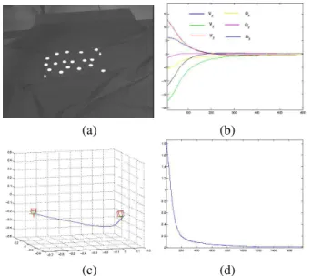
The results obtained using a continuous object where the object is non parallel to the image plane are given on Figure 2. From those results we also note the same exponential decrease behavior obtained either for the features errors (Fig. 2.c) either for the translational velocities (Fig. 2.d.). Furthermore, the obtained 3D camera trajectory (Fig. 2.e.) is a pure straight line.

B. Complex motion

We now consider a complex motions where both trans-lational and rotational motion are involved. More precisely, the displacement to realize is composed of a translation of approximatively 65 cm and of a rotation of approximatively 30 dg. The initial and desired images are given on Figure 3.a and 1.b (non parallel case and discrete object). For that desired position, and after transformation of the visual features, we have: Lk s(s∗ t)=         −1 0 0 0.00 −0.50 0.00 0 −1 0 0.50 −0.0 0.01 0 0 −1 −0.00 −0.01 0 0 0 0 1.49 −0.56 0 0 0 0 1.58 2.50 0 0 0 0 0.11 −0.17 −1         (20)

The obtained interaction matrix is sparse. Its condition number is equal to 3.34 while it is 95.61 using points coordinates. The obtained results are given on Figure 3. Despite the large displacement to realize, we can note the good behavior of the features errors mean and of the camera velocities: they decrease exponentially with no oscillation (see Figure 3.b and Figure 3.d ). The 3D camera trajectory is also satisfactory (see Figure 3.c).

The experimental results using a continuous objet are given on Figure 4. An exponential decrease of the velocities and features errors mean is also obtained. The 3D camera

(6)

(a) (b)

(c) (d)

(e) (f)

(g) (h)

Fig. 1. (a) desired image where the object is parallel to the image plane), (b) desired image where the object is not parallel to the image plane), (c) initial image for a pure translational motion between (a) and (c) ), (d) initial image for a pure translational motion between (b) and (d)), (e) features errors mean, (f) velocities, (g) camera 3D trajectory (object parallel to the image plane) (h) camera 3D trajectory (object non parallel to the image plane).

tory is adequate despite of the large displacement between the desired and the initial position of the camera.

C. Results with a bad camera calibration

We now test the robustness of our approach with respect to modeling errors. In the presented experiment, errors have been added to camera intrinsic parameters (25% on the focal length and 20 pixels on the coordinates of the principal point) and to the object depth for the desired camera position ( bZ∗₌

0.8 m instead of Z∗ _{= 0.5 m). Furthermore, an error equal}

to10 dg has been set in R. The obtained results are given on Figure 5. The behavior of the system is very similar to that of the previous experiment, which validates the robustness of our scheme with respect to such errors.

(a) (b)

(c) (d)

(e)

Fig. 2. Results for a pure translation using a continuous object (when the object is not parallel to the image plane): (a) desired image, (b) initial image, (c) features errors, (d) translational velocities, (e) camera 3D trajectory

(a) (b)

(c) (d)

Fig. 3. Results for a complex motion and using a discrete object: (a) initial image, (b) velocities, (c) camera trajectory, (d) features errors mean

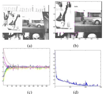
D. Results for complex images

In this paragraph, we present similar experimental results obtained on more complex images (see Figure 6). The con-sidered points have been extracted using Harris detector and tracked using a SSD algorithm. We can note however that

(7)

(a) (b)

(c) (d)

Fig. 4. Results for a complex motion using a continuous object: (a) initial image, (b) camera 3D trajectory, (c) features errors mean, (d) camera velocities.

(a) (b)

(c)

Fig. 5. Results with modeling errors: (a) velocities, (b) features errors mean, (c) camera trajectory.

the plots are more noisy than using simple dots, because of the less accurate points extraction. It is mainly noticeable on theωxandωycomponents of the camera velocity whose value

depends on5th_{order moments (while}_ω

zandυzare not noisy

at all since their value only depend of moments of order 2). Despite this noise, the exponential decrease, the convergence and the stability are still obtained, which proves the validity of our approach. This results can be improved using a sub pixel accuracy image tracker such as Shi-Tomasi algorithm [8].

VI. CONCLUSION

In this paper, we have proposed a new visual servoing scheme based on image moments for objects composed of a set of discrete points. Six features have been designed to

(a) (b)

(c) (d)

Fig. 6. Results for complex images: (a) initial image, (b) desired image, (c) velocities, (d) features errors mean

decouple the camera degrees of freedom, which allows one to obtain a large domain of convergence, a good behavior of the visual features in the image, as well as an adequate camera trajectory.

A new method, based on a virtual camera rotation, has also been proposed to extend the decoupling properties for any desired camera orientation with respect to the considered object. This method is valid either for discrete objects either for continuous objects. The experimental results show the validity and the robustness of our approach with respect to modeling errors. Furthermore, in the case of a discrete objet, our method requires only that the set of points considered in the desired image is the same in the initial and tracked images (no matching between these points is necessary to compute the moments). _R_EFERENCES

[1] F. Chaumette. Potential problems of stability and convergence in image-based and position-image-based visual servoing. In A.S. Morse D. Kriegman, G. Hager, editor, The Confluence of Vision and Control, number 237, pages 66–78. Springer-Verlag, 1998. LNCIS.

[2] P. I. Corke and S. A. Hutchinson. A new partitioned approach to image-based visual servo control. IEEE Trans. on Robotics and Automation, 17(4):507–515, Aug. 2001.

[3] G. Hager and K. Toyoma. The xvision system: A general-purpose substrate for portable real-time vision applications. Computer Vision and Image Understanding, 69(1):23–37, 1997.

[4] C. Harris and M. Stephens. A combined corner and edge detector. In In proceeding of the 4th Alvey Vision Conference, pages 147–151, 1988. [5] S. Hutchinson, G. Hager, and P. Corke. A tutorial on visual servo control.

IEEE Trans. on Robotics and Automation, 12(5):651–670, Oct. 1996. [6] N. Okiyama M. Iwatsuki. A new formulation of visual servoing based on

cylindrical coordinates system with shiftable origin. In IEEE/RSJ IROS, Lausanne, Switzerland, Oct. 2002.

[7] R. Mahony, P. Corke, and F. Chaumette. Choice of image features for depth-axis control in image-based visual servo control. In IEEE/RSJ IROS’02, pages 390–395, Lausanne, Switzerland, Oct. 2002.

[8] J. Shi and C. Tomasi. Good features to track. In CVPR’94, pages 593– 600, Seattle, June 1994.

[9] O. Tahri and F. Chaumette. Application of moment invariants to visual servoing. In IEEE Int. Conf. on Robotics and Automation, ICRA’03, pages 4276–4281, Taipeh, Sep. 2003.