Towards a model for the multidimensional analysis of field data

HAL Id: hal-00527729

https://hal.archives-ouvertes.fr/hal-00527729

Submitted on 14 Dec 2010

HAL is a multi-disciplinary open access

archive for the deposit and dissemination of

sci-entific research documents, whether they are

pub-lished or not. The documents may come from

teaching and research institutions in France or

abroad, or from public or private research centers.

L’archive ouverte pluridisciplinaire HAL, est

destinée au dépôt et à la diffusion de documents

scientifiques de niveau recherche, publiés ou non,

émanant des établissements d’enseignement et de

recherche français ou étrangers, des laboratoires

publics ou privés.

Towards a model for the multidimensional analysis of

field data

S. Bimonte, Myoung-Ah Kang

To cite this version:

S. Bimonte, Myoung-Ah Kang. Towards a model for the multidimensional analysis of field data. 14th

East-European Conference on Advances in Databases and Information Systems, ADBIS 2010, Sep

2010, Novi Sad, Serbia. 15 p. �hal-00527729�

Towards a Model for the Multidimensional Analysis of

Field Data

Sandro Bimonte1_{, Myoung-Ah Kang}2

1_{CEMAGREF, Campus des CEZEAUX,}

63173 AUBIERE, France

2_{LIMOS-UMR CNRS 6158,ISIMA, Blaise Pascal University,Campus des CEZEAUX,}

63173 AUBIERE, France

1_{Sandro.bimonte@cemagref.fr,} 2_{kang@isima.fr}

Abstract. Integration of spatial data into multidimensional models leads to the concept of Spatial OLAP (SOLAP). Usually, SOLAP models exploit discrete spatial data. Few works integrate continuous field data into dimensions and measures. In this paper, we provide a multidimensional model that supports measures and dimension as continuous field data, independently of their implementation.

Keywords: Spatial OLAP, Field data, Spatial Data Warehouses, Multidimensional models

1 Introduction

It has been estimated that about 80% of the data stored in corporate databases integrates geographic information [7]. This information is typically represented according two models, depending on the nature of data: discrete (vector) and field [22]. The latter model represents the space as a continuous field. Fields have to be discretized to be represented into computers according to data input, and data analysis. These representations can be grouped into two categories: incomplete and complete. Incomplete representations store only some points and need supplementary functions to calculate the field in non-sampled areas. Complete representations associate estimated values to regions and assume that this value is valid for each point in the regions (raster). Fields are very adapted for modeling spatial phenomena such as pollution, temperature, etc. They allow a point by point analysis through the Map Algebra operators [16] [22].

In order to benefit from Data warehousing and OLAP decision support technologies [11] also in the context of spatial data, some works extended them leading to the concept of Spatial OLAP (SOLAP), which integrates OLAP and Geographic Information Systems (GIS) functionalities into a unique framework [2]. As for the model underlying SOLAP systems, several research issues from theoretical and implementation point of view have risen. Indeed, several works focus on indexing [20] and visualization techniques [6]. Motivated by the relevance of a formal

Author-produced version of the paper published in Advances in Databases and Information Systems

14th East European Conference, ADBIS 2010, Novi Sad, Serbia, September 2024, 2010, Proceedings, Series: Lecture Notes in Computer Science, Vol. 6295 -Catania, Barbara; Ivanovic, Mirjana; Thalheim, Bernhard (Eds.) 2010, ISBN 978-3-642-15575-8

representation of SOLAP data and operators, some spatio-multidimensional models based on vector data have been defined (a review can be found in [4]). Few works consider field data into multidimensional models [1], [23] and [15]. These models present some limitations that do not allow fully exploiting continuous field data into OLAP from these points of view: aggregation functions, hierarchies based on field, and independence of field data implementation. Thus, in this paper we propose a spatio-multidimensional model integrating field data.

The reminder of this paper is organized as follows: Section 2 recalls fundamentals of spatial analysis techniques, and existing SOLAP models for field data. Our model is proposed in the Section 3. Finally, in Section 4 conclusions and future work are presented.

2 Related work

The term Map Algebra was first introduced in [22] to describe operators on raster data (complete field data). Map Algebra operators are classified according to the number of grids and cells involved. Local operators apply a mathematical or logical function to the input grids, cell by cell. Focal operators calculate the new value of each cell using neighboring cells values of the input grid. Zonal operators calculate new values as a function of the values of the input grid which are associated with the zone of another grid, called zone layer. An extension of the Map Algebra (Cubic Map Algebra) to the temporal dimension is presented in [16]. The authors redefine Map Algebra operators on a cube of cells whose coordinates are three-dimensional. Then, the sets of operators are modified accordingly as shown on Figure 1. In [5] the authors define an algebraic model for field data. This framework provides a formal definition of Map Algebra operators independent of their implementation. Along this line, the work of [8] formally describes how Map Algebra fundamentals can be used for image manipulation. Finally, Map Algebra has been defined also for incomplete field data such as Voronoi tessellations [13]. Indeed, "Map Algebra obliges analysts to organize reality according to a particular data structure (raster) instead of allowing making the reality suggest the most adequate data structure for the analysis" [10].

On the other hand, the integration of spatial data into data warehousing and OLAP systems leads to the concept of Spatial OLAP (SOLAP). SOLAP is based on the spatial multidimensional model that defines spatial dimensions and spatial measures. In particular, a spatial dimension is a classical dimension whose levels contain spatial attributes. This allows for visualizing measures on maps to discover (spatial) relations and unknown patterns. According to the vector model, a spatial measure is defined as a set of geometries and/or the result of spatial operators [2] [14]. Some spatial multidimensional models, based on the vector model, have been proposed [4]. Despite of the significant analysis power of field data and its associated spatial analysis operators, only few works address this issue. [15] extends the concepts of spatial dimension to informally define "spatial matrix (raster) dimension" where at least one level represents raster data. Then, a member is a cell of the raster. Moreover, she introduces also the concept of "matrix cube" where each fact is associated to a cell of the raster data with its attributes. Aggregation functions are Map Algebra operators

(local, focal and zonal). The author limits field data to raster. By this way, the work loses in terms of abstraction for field data. Indeed, Map Algebra has been defined also on other forms of representation of field data such as Voronoi tessellation [13], and terrain representations, such as TIN, that could be very useful for understanding and analyzing multidimensional data [6].

(a) (b) (c)

(d) (e)

Figure 1. Map Algebra: a) local, b) focal, c) zonal [22], Cubic Map Algebra: d) focal, e) zonal [16].

Hence, [23] proposes a conceptual multidimensional model for taking into account field data independently of their implementation. They define a "field measure" as a value that changes in space and/or time. The model limits aggregation functions for field measure to local Map Algebra functions. They also introduce a "field hierarchy" when a level is a field data that is not linked to facts. Consequently, it is not possible to have field measures at different granularities, which are mandatory for spatial analysis [21]. Finally [1] defines the concept of "continuous cube" when spatial dimensions are composed of infinite spatial members whose associated numerical measures are calculated using interpolation functions, as they use an incomplete representation of spatial members. This model does not allow introduce field data as measures and in hierarchies.

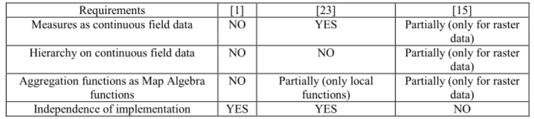
Therefore, a formal model is necessary to create the foundation for a framework for the multidimensional analysis of field data as dimensions (field hierarchies) and measures. Table 1 shows the requirements for this model and how existing works address them. As shown in table 1, there is no existing model that supports all of these requirements. This is the reason why we propose a new SOLAP model in this paper.

Table 1: Requirements for spatial multidimensional model for continuous field data.

Requirements [1] [23] [15] Measures as continuous field data NO YES Partially (only for raster

data) Hierarchy on continuous field data NO NO Partially (only for raster

data) Aggregation functions as Map Algebra

functions

NO Partially (only local functions)

Partially (only for raster data) Independence of implementation YES YES NO

3 Spatio-multidimensional model for field data

Before introducing our model we present a SOLAP application for monitoring earthquakes in Italian regions. Spatial analyst wants answer to queries like this: “Where were earthquakes, and what was their intensity per region at different scales (resolutions)?”. This SOLAP application presents a measure that is a field object representing the earthquakes, a temporal dimension, and a spatial dimension that represents terrain models of Italian regions at different scales.

3.1 Geographic data model

In this section, we provide a uniform representation for field and vector data, which are used by the multidimensional model to define measures and dimensions members.

An Object represents an object of the real world described by some alphanumeric attributes. It is used in the model to represent levels and members (Sec. 3.2).

Definition 1. Object

An Object Structure Se is a tuple 〈a1, …an〉 where ∀ i ∈ [1,…n] ai is an attribute

defined on a domain dom(ai)

An Instance of an Object Structure Se is a tuple 〈val(a1),…val(an)〉 where ∀ i ∈ [1,…n]

val(ai) ∈ dom(ai)

We denote by 'I(Se)' the set of instances of Se

A Geographic Object extends an Object to represent geographic information according to the vector model. Indeed, a Geographic Object [3] is a geometry (geom) and an optional set of alphanumeric attributes ([a1, …an]) whose values are associated

to the whole geometry according to the vector model (Figure 2a). Definition 2. Geographic Object

Let g ⊂ R2 i.e.a subset of the Euclidian space. An Object Structure Se = 〈geom, [a1,

…an]〉 is a Geographic Object Structure if the domain of the attribute geom is a set of

geometries: dom(geom)∈ 2g

Example 1.

The geographic object structure representing Italian regions is Sregion=〈geom, name〉

where 'geom' is the geometric support, and 'name' is the name of the region. An instance of Sregion is t2 = 〈plo, Lombardia〉 where 'plo' is the geometry of the region

Lombardia (Figure 2a).

p2

f₂(x;y)=12

(a) (b)

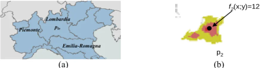
Figure 2: a) Italian regions: Instances of Sregion, b) Earthquakes: an instance of Searthq.

According to [13] fields are geographic objects with a function that maps each point of their geometry to an alphanumeric value. This definition allows for representing field data independently of their implementation (complete/incomplete) (Field Object). Thus, A Field Object extends a Geographic Object with a function that associates each point of the geometry to an alphanumeric value. In this way, a Field Object allows for representing geographic data according to the field and the vector model at the same time ("Independence of implementation" requirement of Table 1).

Definition 3. Field Object

Let Se = 〈geom, field, [a1, …an]〉 a Geographic Object Structure. Se is a Field Object

Structure if the domain of the attribute field is a set of functions defined on m sub-sets of points of geom having values in an alphanumeric domain domfield : dom(field)= {f1 …

fm}

An Instance of an Field Object Structure Se is a tuple 〈g, fj, val(a1),…val(an)〉 where: − ∀ i ∈ [1,…n] val(ai) ∈ dom(ai), g ∈ dom(geom)

− fj : g → domfield and fj ∈ {f1 , …, fm}

We note 'field support' the input domain of fj

Example 2.

The field object structure representing earthquakes is Searthq=〈geom, intensity〉 where

'geom' is the geometric support, and 'intensity' is a set of functions defined on 'geom' with values in R. 'intensity' represents the intensity of the earthquake. An instance of Searthq is t2 = 〈p2, f2〉 where p2 is a geometry and f2 represents the intensity of the

earthquake on the 11-1999 in Lombardia. f2 is defined on each point of p2 with values

in R, for example f2 (x;y) = 12 (Figure 2b).

By the same way, we can define a field object structure to represent terrain models of Italian regions at different scales by adding to the geographic object Sregion the field

attribute representing terrain elevation.

Piemonte

Lombardia

Emilia-Romagna plo

3.2 Spatio-multidimensional model for field data

A spatio-multidimensional model organizes data using the concepts of dimensions composed of hierarchies, and facts described by measures. An instance of the spatio-multidimensional model is a hypercube. Section 3.2.1 presents the concepts of dimensions, facts, and measures, and Section 3.2.2 formalizes cuboids.

3.2.1 Hierarchies and facts

According to [3] a spatial hierarchy organizes vector objects in a hierarchical way. Formally, a Spatial Hierarchy organizes the Geographic Objects [3] (i.e. vector objects) into a hierarchy structure using a partial order ≤h where Si ≤h Sj means that Si

is a less detailed level than Sj. An instance of a hierarchy is a tree (<h) of instances of

Geographic Objects (spatial members). Then, measures are aggregated according to the groups of spatial members defined by the tree <h.

Hence, in this work we define a Field Hierarchy as a hierarchy of field objects. For that, we extend the spatial hierarchy by defining a tree (<f) on the geometric

coordinates (field supports) of the spatial members represented by field objects ("Hierarchy on continuous field data" requirement of Table 1). By this way it is possible to visualize field objects at different scales or resolutions (Figure 4). Moreover, the alphanumeric values associated to each point of the field measures are aggregated according to the groups of coordinates of spatial members defined by the tree <f . By

this way, our model uses the continuous representation of spatial members (Field Objects) to aggregate measure, allowing visualizing field measures at different scales or resolutions (see Figure 6b).

Definition 4. Field Hierarchy

A Field Hierarchy Structure, Hh, is a tuple 〈L h, h, h, ≤h〉 where:

− h, h, are of Field Object Structures, and Lh is a set of Field Object Structures − ≤h is a partial order defined on L h, h, h as defined in [3]

An Instance of a Field Hierarchy Structure Hh is two partial orders: <h and <f such

that:

− <h is defined on the instances of L h, h, h as defined in [3]

We note <h 'geographic objects order'

− <f is defined on the field supports of the instances of L h, h, h such that:

- if coodi <f coodj then Si ≤h Sj , where coodi belongs to a field support of an

instance of Si , and coodj belongs to a field support of an instance of Sj, (coodi and

coodj are geometric coordinates)

-∀ coodi which does not belong to the field supports of the instances of h, ∃ one

coodj belonging to the field support of an instance of Sj such that coodi <f coodj -∀ coodi which does not belong to the field supports of the instances ofh, ∃ coodj

We note <f 'field objects order'

The set of leafs of the tree represented by <h with root ti are denoted as leafs(Hh, ti).

The set of leafs of the tree represented by <f with root coodi are denoted as

leafsFieldSupport(Hh, coodi).

Example 3.

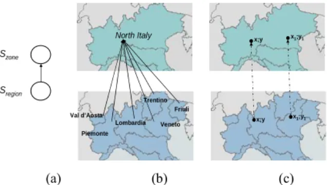
The field hierarchy structure representing the administrative dimension that groups regions into zones is Hlocation = 〈Llocation, Sregion, Sall_location, ≤location〉 where Llocation =

{Szone} and (Sregion ≤location Szone). Sregion and Szone are the spatial levels of the hierarchy

(Figure 3a). An example of instance of Hlocation is shown on Figure 3b and 3c. We can

notice two trees: the geographic objects order that is represented by black lines (Figure 3b), and the field objects order, which is represented by dashed lines (Figure 3c). Sregion Szone North Italy Lombardia Piemonte Val d’Aosta Veneto Friuli Trentino x;y x;y x1;y1 x1;y1 (a) (b) (c)

Figure 3: Field hierarchy grouping regions into zones, a) Schema, b) Hierarchical relationships between geographic objects, c) Hierarchical relationships between geometric coordinates.

Example 4.

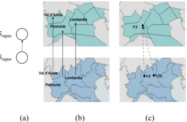
The hierarchy structure representing the terrain models of Italian regions at different resolutions is Hregres =〈Lregres, Sregion, Sall_regres, ≤regres〉 where Lregres = {Sregres} and (Sregion

≤regres Sregres ) (Figure 4a). Its instance is shown on Figure 4b and Figure 4c. Note that a

geometric coordinate at the coarser resolution is associated with a set of geometric coordinates at the most detailed resolution (Figure 4c). For example, this hierarchy can be defined using the bilinear interpolation algorithms used for changing resolution for raster data at different scales.

Sregion Sregres Lombardia Piemonte Val d’Aosta Lombardia Piemonte Val d’Aosta x;y x;y x1;y1 (a) (b) (c)

Figure 4: Field hierarchy representing regions at different scales, a) Schema, b) Hierarchical relationships between geographic objects (geographic objects order), c) Hierarchical relationships between geometric coordinates (field objects order).

Once we have introduced the concepts of measures, and hierarchies for field data, we present the concept of Field Cube. A Field Cube Structure represents the spatio-multidimensional model schema where a field object is used as measure that is analyzed according classical hierarchies and one field hierarchy ("Measures as continuous field data" requirement of Table 1). Note that without losing in generalization, we suppose to have only one spatial dimension and one field measure to simplify the formalism of the model. In the same way, we do not introduce numerical measures as they can be simply represented using numeric attributes as defined in [3]. An instance of a field cube structure represents the fact table or the basic cuboid of the lattice cuboids.

Definition 5. Field Cube

A Field Cube Structure, FCc , is a tuple 〈H1,…Hn, FieldObject〉 where:

- H1 is a Field Hierarchy Structure (Spatial dimension)

- ∀ i ∈ [2,…n] Hi is a Hierarchy Structure (Dimensions)

- FieldObject is Field Object Structure (Field measure)

An Instance of a Field Cube Structure FCc , I(FCc), is a set of tuples {〈tb1,…tbn, tbf〉}

where:

- ∀ i ∈ [1,…n] tbi is an instance of the bottom level of Hi (i) (Most detailed levels

members)

- tbf is an instance of FieldObject (Field measure value)

Example 5.

The field cube structure of our case study is FCearthq = 〈Hregtres, Htime, Searthq〉. Hregtres is

the field hierarchy (the spatial dimension), Htime is the temporal dimension, and Searthq

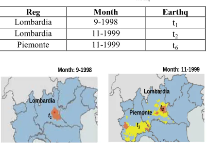
is the field measure. It allows answering previous formulated query “Where were earthquakes, and what was their intensity per region at different scale (resolutions)?”. Table 2 shows the instance of FCearthq. Its cartographic representation is shown on

Table 2: Instance of FCearthq.

Reg Month Earthq

Lombardia 9-1998 _t1 Lombardia 11-1999 _t2 Piemonte 11-1999 _t6 Lombardia Piemonte t2 t3 Month: 11-1999 Lombardia t1 Month: 9-1998

Figure 5: Cartographic representation of the instance of FCearthq.

3.2.2 Hypercube

The instance of the spatio-multidimensional model is a hypercube. A hypercube can be represented as a hierarchical lattice of cuboids [9]. The most detailed cuboid contains detailed measures (basic cuboid). Other cuboids contain aggregated measures. Then, cuboids are represented by levels and (aggregated) measures values (Sec. 3.2.2.2). How field measures are aggregated from fact table data (basic cuboid) to represent non-basic cuboids is presented in Sec. 3.2.2.1.

3.2.2.1 Aggregation of field measures

The aggregation of field measures is defined by means of:

- For the geometric support: spatial aggregation,

- For alphanumeric attributes: alphanumeric aggregations

- For the field attribute:

- Local Map Algebra, or focal/zonal map cubic algebra operator when aggregating on the non-field hierarchies

- Alphanumeric aggregation when aggregating on the field hierarchy

Indeed aggregation of field measures is done in two steps. In the first step we aggregate along the non-field hierarchies, and then along the field hierarchy.

3.2.2.1.1 Aggregation on non-field hierarchies

Definition 6. Spatial aggregation

Let G the geometric attribute. Its aggregation is defined by means of a function OG

that has as input n geometries of the attribute G, and that returns one geometry: OG : dom(G)×… × dom(G) → 2g where g is a subset of the Euclidian Space R2

Definition 7. Alphanumeric aggregation

Let A be an alphanumeric attribute. Its aggregation is defined by means of a function OA that has in input n values of the attribute A, and that returns one value of the

attribute A:

OA : dom(A)×… × dom(A) → dom(A)

On non-field hierarchies, the aggregation of the field attribute is defined by means of a function (OF) that takes as input a set of functions representing the field attributes

values (f1…fn), and it returns a new function (f1n). This function is defined on the field

support of f1…fn, and the value of each point (f1n(x;y)) is calculated by applying a

alphanumeric function OA to the values of the other functions (OF (f1(x;y)…fn(x;y))).

Then, OF represents a map/map cubic algebra operator that is specialized in local,

focal or zonal by means of the OA function. Indeed, OA is applied point by point for

local map function, or to sets of coordinates defined by the functions Neighborhood(x;y) and Zone(FieldObjects, (x;y)) for focal map cubic and zonal map cubic operators respectively (("Aggregation functions as Map/Map Cubic Algebra functions " requirement of Table 1)).

Definition 8. Aggregation of the Field attribute on non-field hierarchies using Map Algebra and Cubic Map algebra functions

Let F be a field attribute, and f1…fn functions of the domain of F with g as field

support (without loss of generality, we suppose the f1…fn have the same field support)

f1 : g → domF … fn : g → domF, and f1…fn∈ dom(F).

Let OA be an alphanumeric aggregation

Then, the aggregation of F is defined by means of a function OF that takes as input

f1…fn, and that returns a function f1n defined on g and having values in domF (f1n : g →

domF) (f1n = OF (f1…fn)) such that:

- using Local operator:

f1n (x; y) = OA(f1(x;y), …, fn(x;y)) for each point (x;y) of g

- using Cubic Focal operator:

f1n (x; y)= OA(f1 (Neighborhood(x;y))…fn(Neighborhood(x;y))) for each point (x;y) of g

where:

Neighborhood(x;y) is a function that returns the neighbourhood points of (x;y),

- using Cubic Zonal operator:

f1n (x; y)= OA(f1(Zone(FieldObjects,(x;y))…fn(Zone(FieldObjects,(x;y))) for each point (x;y)

Zone(FieldObjects, (x;y)) is a function that takes as input a set of Field Objects and a point, and it returns the neighbourhood points of (x;y)that belong to the zone indentified by the FieldObjects on this point.

Definition 9. built non-field (Figure 7)

Let tbf1,…tbfk and tnf instances of the field object structure Se = 〈geom, field, [a1, …am]〉

Let ONF, called non-field aggregation mode, a set of aggregation functions:

- OG the spatial aggregation for geom

- O1... Om the alphanumeric aggregations for a1, …am

- OF the Map Algebra/Map Cubic Algebra aggregation for field

We say that tnf is built non-field from tbf1,…tbfk using ONF if:

- tnf.geom = OG (tbf1. geom,…, tbfk.geom)

- ∀ i ∈ [1,…m] tnf .ai. = Oi (tbf1. ai,…, tbfk. ai)

- tnf .field = OF(tbf1.field,…, tbfk. field)

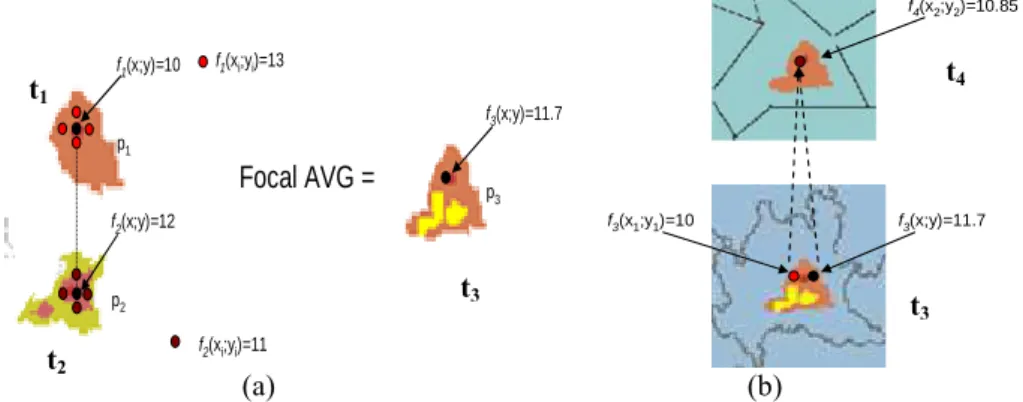
Example 6.

Let an instance of Searthq t1 = 〈p1, f1〉 where p1 is a geometry and f1 represents the

intensity of the earthquake on the 9-1998 in Lombardia. It is defined on each point of p1 with values in R. For example f1 (x;y) = 10 (Figure 6a). To aggregate the field

attribute intensity on the temporal dimension, we use a cubic focal operator AVG. Therefore the result of the aggregation of f1 and f2 on (x;y) by taking into account

neighbours of (x;y) is f3 (x;y)= ((13*4+10)+(11*4+12))/10=11.7 (we suppose that the

values of neighbourhood points of (x;y) of t1 and t2 are 10 and 12 respectively) (Figure

6a). We suppose that we apply the geometric union for geometry.

Then, t3 is built non-field from t1 and t2. t3 is an aggregated measure of the cuboid

defined by the century level of the temporal dimension (see Table 3).

Table 3: Instances of the cuboid defined by the century level of the temporal dimension.

Region Century Earthq

Lombardia 900 t3

Piemonte 900 t6

Then, as a field measures is mapped also on spatial dimensions, then a particular aggregation must be provided taking into account the field hierarchy in order to allow the visualization of field measures at different resolutions or scales.

3.2.2.1.2 Aggregation on the field hierarchy

The aggregated measures of a cuboid defined by coarser spatial levels are the aggregation of the (aggregated) measures of the cuboids defined by non-spatial levels. Definition 10. built field (Figure 7)

Let t1_{nf,…, t}v

nf and tf be instances of the field object structure Se〈geom, field, [a1, …am]〉.

Let OF, called field aggregation mode, a set of aggregation functions:

- O1... Om the alphanumeric aggregations for a1, …am

- OA the alphanumeric aggregation for field

We say that tf is built field from t1nf,…, tvnf using OF if:

- tf .geom = OG (t1nf. geom,…, tvnf.geom)

- ∀ i ∈ [1,…m] tf .ai. = OG (t1nf. ai,…, tvnf. ai)

- tf .field (x; y)= OA (f1(x1;y1), …, fm(xm;ym)) wheref1, …, fmbelong to t1nf.field , … tvnf.field,

for each point (x;y) of the field support of field

p1 f1(x;y)=10 p2 f₂(x;y)=12 f1(xi;yi)=13 f2(xi;yi)=11 p3 f3(x;y)=11.7 Focal AVG = f₃(x;y)=11.7 f₃(x₁;y₁)=10 f₄(x₂;y₂)=10.85 (a) (b)

Figure 6: a) Aggregation on the "intensity" field attribute on the temporal dimension, b) Aggregation on the "intensity" field attribute on the field hierarchy.

Example 7.

In order to visualize the measure at different resolutions, we aggregate on the Field Hierarchy Hregres applying the average. Then f4(x;y) =

AVG(leavesFieldSupport(Hdeptres, (x2;y2))) = AVG(f3(x;y), f3(x1;y1)) = (10+11.7)/2 =

10.85 (Figure 6b). Then, t4 is built field from t3. t4 is an aggregated measure of the

cuboid defined by the century and regres levels (see Table 4).

Table 4: Instance of FCearthq.

Regres (region at scale 1:1.000)

Century Earthq

Lombardia 900 t4

Piemonte 900 t5

3.2.2.2 Cuboids of field data

Once described how the measures of the different cuboids are related by aggregation functions, in this section we formalize the concept of cuboid. In particular, a cuboid schema, noted Field View Structure, is composed by a set of levels, a non-field aggregation mode, and a field aggregation mode. An instance of a field view structure is a set of tuples composed of a member for each level and a (aggregated) field measure value. The aggregated field measure value on the spatial

t1

t2

t3 _t

3

dimension (tf) is obtained aggregating measures (t1nf …, tvnf) obtained after the

aggregation on the non-spatial dimensions of detailed measures (tbf1 …, tbfk) as shown

on Figure 7.

Definition 11. Field View

A Field View Structure Vv is a tuple 〈FCc, L, ONF, OF〉 where:

- FCc=〈H1,…Hn, FieldObject〉 is a Field Cube Structure (Spatio-multidimensional

model schema)

- L is a tuple 〈S1,…Sn〉 where∀ i ∈ [1,…n] Si is a level of Hi (Levels that define the

cuboid)

- ONF is a non field aggregation mode (Aggregation functions used on non-spatial dimensions)

- OF is a field aggregation mode (Aggregation functions used on the spatial dimension)

An Instance of a field view Structure is a set of tuples {〈t1,…tn, tf〉} where: - ∀ i ∈ [1,…n] ti is an instance of Si (Dimensions members)

- tf is: ((aggregated) field measure on spatial dimension, Figure 7 - see Table 4 for

an example)

- an instance of FieldObject

- built field from t1_{nf,…, t}v_{nf using OF where ((aggregated) field measures on}

non-spatial dimensions, Figure 7 - see Table 3 for an example):

- tf.field (x;y)= OF.OA (f1(x1;y1), …, fm(xm;ym)) for each point (x;y) of its field

support where:

- (x1_;y1_{), …, (x}m_;ym_{) belong to leafsFieldSupport(H1, (x;y))}

- f1 _{, …, f}m _{belong to t}1_{nf.field,…, t}v_nf.field

- Eachtj_{nf is built non field from tb}j_{f1, …, tb}j_{fk using ONF where (Non aggregated}

field measures, Figure 7 - see Table 2 for an example):

- tbj_{f1, …, tb}j_{fk are the measure values of the tuples of I(FCc)} 〈_tbj_1,

tb1_{2… tb}1_{n, tb}j_f1〉, ...,〈_tbj_{1, tb}k_{2… tb}k_{n, tb}j_fk〉 _where:

- ∀ i ∈ [2,…n] tb1_{i … tb}k_{i = leafs(Hi, ti)}

- tbj

1 belongs to leafs(H1, t1)

Example 8.

The Field View Structure representing earthquakes per region at the scale 1:10000 and per century is Vearthq = 〈FCearth, 〈Scentury, Sregres〉, 〈Union, Focal-Avg〉, 〈Union, Avg〉〉.

Table 4 shows its instance.

4 Conclusion and future work

Integration of spatial data into multidimensional models leads to the concept of SOLAP. SOLAP models exploit the discrete representation of spatial data. Few works integrate continuous field data into dimensions and measures. In this paper, motivated by the relevance of a formal representation of SOLAP data, we provide a multidimensional model that considers field data independently form their

implementation, as measures and dimensions. In particular we provide a unique data model for vector and field data (Geographic and Field Objects). We provide a formal representation of the spatio-multidimensional model schema (Field Cube: Field Hierarchy and Field Measures) and the associated hypercube's cuboids (Field View). Actually, we are working on the formal definition of SOLAP operators that allows the navigation between the cuboids (roll-up/drill-down), and slicing the cuboids (slice). We plan to work on the implementation of the model in a ROLAP architecture. This implies the definition of: (i) query languages for OLAP server [18] for field data [12], (ii) indexes [20] and pre-aggregation techniques [19] for spatial data warehouses using field dimensions and measures, and (iii) interactive field maps [17] for SOLAP clients.

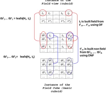
tfis built field from t1

nf… tvnfusing OF

t1

nfis built non field from tb1 f1,… tb1fk using ONF tb1 1… tbv1= leafs(H1, t1) tb1 2… tbk2= leafs(H2, t2) Instance of the Field Cube (basic

cuboid) Instance of the Field view (cuboid)

Figure 7: Instance of a Field View Structure

References

[1] Ahmed, T., Miquel, M.: Multidimensional Structures Dedicated to Continuous Spatiotemporal Phenomena. In: 22th British National Conference on Databases. LNCS, vol. 3567 pp. 29-40. Springer, Heidelberg (2005)

[2] Bédard, Y., Han, J.: Fundamentals of Spatial Data Warehousing for Geographic Knowledge Discovery. Geographic Data Mining and Knowledge Discovery. Taylor & Francis, New York, USA (2009)

[3] Bimonte, S., Gensel, J., Bertolotto, M.: Enriching Spatial OLAP with Map Generalization: a Conceptual Multidimensional Model. In: IEEE International Workshop on Spatial and Spatiotemporal Data Minin, pp. 332 – 34. IEEE CS Press (2008)

[4] Bimonte, S., Tchounikine, A., Miquel, M., Pinet, F.: When Spatial Analysis Meets OLAP: Multidimensional Model and Operators. International Journal of DataWarehousing and Mining (to appear)

[5] Câmara, G., De Freitas, U., Cordeiro, J.: Towards an algebra of geographical fields. In: Brazilian Symp. on computer graphics and image processing, Anais, Curitiba, pp. 205–212 (1994)

[6] Di Martino, S., Bimonte, S., Bertolotto, M., Ferrucci; F.: Integrating Google Earth within OLAP Tools for Multidimensional Exploration and Analysis of Spatial Data. In: ICEIS 2009. LNBIP, vol. 24, pp. 940-951. Springer, Heidelberg (2009)

[7] Franklin, C.: An Introduction to Geographic Information Systems: Linking Maps to databases. Database, 15(2), 13-21 (1992)

[8] Gutierrez, A., Baumann, P.: Modeling Fundamental Geo-Raster Operations with Array Algebra. In: IEEE International Workshop on Spatial and Spatiotemporal Data Mining, pp. 607-612. IEEE CS Press (2007)

[9] Harinarayan, V., Rajaraman, A., Ullman, J. D.: Implementing Data Cubes Efficiently. In: ACM SIGMOD International Conference on Management of Data, pp. 205-216. ACM Press, New York (1996)

[10] Kemp, K.: Environmental Modeling with GIS: A Strategy for Dealing with Spatial Continuity. Technical Report 93-3. National Center for Geographic Information and Analysis, University of California, Santa Barbara, USA (1993)

[11] Kimball, R.: The Data Warehouse Toolkit: Practical Techniques for Building Dimensional Data Warehouses. John Wiley & Sons, New York, USA (1996).

[12] Laurini, R., Gordillo, S.: Field Orientation for Continuous Spatio-temporal Phenomena. In: International Workshop on Emerging Technologies for Geo-based Applicatons. pp. 77-101 Swiss Federal Institute of Technology, Lausanne (2000)

[13] Ledoux, H., Gold., C.M.: A Voronoi-based Map Algebra. In: 12th International Symp. on Spatial Data Handling, pp. 117-131. Springer, Heidelberg (2006)

[14] Malinowski, E., Zimányi, E.: Advanced Data Warehouse Design From Conventional to Spatial and Temporal Applications. Springer, Heidelberg (2008)

[15] McHugh, R.: Intégration De La Structure Matricielle Dans Les Cubes Spatiaux. Université Laval (2008)

[16] Mennis, J., Viger, R., Tomlin, C.D.: Cubic Map Algebra functions for spatio-temporal analysis. Cartography and Geographic Information Systems, 30(1), 17-30 (2005)

[17] Plumejeaud, C., Vincent, J., Grasland, C., Bimonte, S., Mathian, H., Guelton, S., Boulier, J., Gensel, J.: HyperSmooth, a system for Interactive Spatial Analysis via Potential Maps. In: International Symposium on Web and Wireless Geographical Information Systems. LNCS, vol. 5373, pp. 4-16. Springer, Heidelberg (2008)

[18] Silva, J., Castro Vera, A.S., Oliveira, A.G., Fidalgo, R., Salgado, A.C., Times, V.C.: Querying geographical data warehouses with GeoMDQL. In: Brazilian Symposium on Databases, pp. 223–237 (2007)

[19] Stefanovic, N., Han, J., Koperski, K.: Object-Based Selective Materialization for Efficient Implementation of Spatial Data Cubes. IEEE Transactions on Knowledge and Data Engineering, 12 (6), 938-958 (2000)

[20] Tao, Y., Papadias, D.: Historical spatio-temporal aggregation. ACM Trans. Inf. Syst., 23(1), 61-102 (2005)

[21] Timpf, S., Frank, A. U.: Using hierarchical spatial data structures for hierarchical spatial reasoning. In: Spatial Information Theory - A Theoretical Basis for GIS.LNCS, vol. 1329, pp 69-83. Springer, Heidelberg (1992)

[22] Tomlin, C.D.: Geographic Information Systems and Cartographic Modeling. Prentice Hall, Englewood Cliffs, NJ (1990)

[23] Vaisman, A., Zimányi, E.: A multidimensional model representing continuous fields in spatial data warehouses. In: 17th ACM SIGSPATIAL International Symp. on Advances in Geographic Information Systems, pp. 168-177. ACM Press, New York, USA (2009)