HAL Id: hal-01221316
https://hal.inria.fr/hal-01221316v3
Submitted on 8 Mar 2016
HAL is a multi-disciplinary open access
archive for the deposit and dissemination of
sci-entific research documents, whether they are
pub-lished or not. The documents may come from
teaching and research institutions in France or
abroad, or from public or private research centers.
L’archive ouverte pluridisciplinaire HAL, est
destinée au dépôt et à la diffusion de documents
scientifiques de niveau recherche, publiés ou non,
émanant des établissements d’enseignement et de
recherche français ou étrangers, des laboratoires
publics ou privés.
Biomedical image segmentation using geometric
deformable models and metaheuristics
Pablo Mesejo, Andrea Valsecchi, Linda Marrakchi-Kacem, Stefano Cagnoni,
Sergio Damas
To cite this version:
Pablo Mesejo, Andrea Valsecchi, Linda Marrakchi-Kacem, Stefano Cagnoni, Sergio Damas.
Biomedi-cal image segmentation using geometric deformable models and metaheuristics. Computerized MediBiomedi-cal
Imaging and Graphics, Elsevier, 2015, 43, pp.167-178. �10.1016/j.compmedimag.2013.12.005�.
�hal-01221316v3�
Biomedical Image Segmentation using
Geometric Deformable Models and Metaheuristics
Pablo Mesejoa, Andrea Valsecchib, Linda Marrakchi-Kacemc,d, Stefano Cagnonia, Sergio Damasb aIntelligent Bio-Inspired Systems laboratory (IBISlab),
Department of Information Engineering,
University of Parma, Viale G.P. Usberti 181a, 43124, Parma, Italy
bEuropean Center for Soft Computing,
C/ Gonzalo Guti´errez Quir´os, s/n - 3aplanta, 33600 Mieres, Spain cNeurospin, CEA, Gif-Sur-Yvette, France
dCRICM, UPMC Universit´e Paris 6, France
Abstract
This paper describes a hybrid level set approach for medical image segmentation. This new geometric deformable model combines region- and edge-based information with the prior shape knowledge introduced using deformable reg-istration. Our proposal consists of two phases: training and test. The former implies the learning of the level set parameters by means of a Genetic Algorithm, while the latter is the proper segmentation, where another metaheuristic, in this case Scatter Search, derives the shape prior. In an experimental comparison, this approach has shown a better performance than a number of state-of-the-art methods when segmenting anatomical structures from different biomedical image modalities.
Keywords: Image Segmentation, Deformable Models, Deformable Registration, Genetic Algorithms, Scatter Search
1. Introduction
Image segmentation is commonly defined as the parti-tioning of an image into non-overlapping regions that are homogeneous with respect to some visual feature, such as color or texture [1]. In many medical imaging applica-tions, segmentation algorithms play a crucial role by auto-matically identifying anatomical structures and other re-gions of interest. Such algorithms are nowadays in the core of multiple tasks, like quantification and measurement of tissue volumes, localization of pathologies or computer-integrated surgery. It is important to highlight that man-ual segmentation is not only tedious and time consuming but, sometimes, also inaccurate, hence the importance of developing automatic and accurate segmentation methods. In particular, medical imaging segmentation is usually challenging due to poor image contrast, noise, diffuse or-gan/tissue boundaries, and artifacts. These problems can cause considerable difficulties when applying traditional segmentation techniques, such as edge detection or thresh-olding. Consequently, an intelligent way of proceeding is to incorporate as much prior knowledge as possible about the particular object and image modality to segment. To
Email addresses: [email protected] (Pablo Mesejo), [email protected] (Andrea Valsecchi), [email protected] (Linda Marrakchi-Kacem), [email protected] (Stefano Cagnoni),
[email protected] (Sergio Damas)
address these difficulties, deformable models have been ex-tensively studied and widely used in medical image seg-mentation with interesting results [2, 3].
A single source of prior knowledge is usually not enough to satisfactorily tackle medical image segmentation prob-lems. Therefore, the development of hybrid approaches combining different sources of information has been a ma-jor focus in the field of image segmentation [4, 5, 6]. In this work, the search/learning abilities of metaheuristics and the capability of geometric deformable models to han-dle topological changes are combined. Three sources of information (a region term, a shape prior, and an edge term) are used to accurately segment the organs of inter-est in different medical image modalities: microscopy, X-ray computed tomography (CT), and magnetic resonance imaging (MRI). In our proposal, metaheuristics [7] have capital importance in two stages. First, during the train-ing process of the new model, the tuntrain-ing of the parameters is carried out by a Genetic Algorithm [8]. Second, in the proper segmentation stage, the shape prior is obtained by a deformable registration process guided by Scatter Search [9].
Every image modality has its own peculiarities, thus the training phase allows our model to learn the most suit-able parameters for a specific modality/anatomical district using few images as paradigmatic examples. In turn, the segmentation phase uses only one manually segmented ref-erence image to generate the prior shape knowledge that will guide, together with the region- and edge-based terms,
the evolution of the moving contour.
To assess the quality of the new approach, we devel-oped an experimental comparison including seven state-of-the-art segmentation methods. The study was carried out on four different datasets, for a total of 22 microscopy, 11 MR, and 5 CT images.
This paper is structured as follows: in section 2 we pro-vide the theoretical foundations necessary to understand our work. In section 3, a general overview of the method is presented, providing details about the different terms used in our deformable model. Finally, section 4 presents the results and the statistical analysis of the experimental comparison, followed, in section 5, by some final remarks and a discussion about possible future developments.
2. Theoretical Background
In this section, an overview of the main techniques ap-plied in our approach (geometric deformable models, im-age registration and metaheuristics) and previous related work are presented.
2.1. Deformable Models
The term “deformable models” (DMs) was first used in the late eighties [10] with reference to curves or surfaces, defined within the image domain, that are deformed under the influence of “internal” forces, related with the curve features, and “external” forces, related with the features of the image regions surrounding the curve. Internal forces enforce regularity constraints and keep the model smooth during deformation, while external forces are defined to attract the model toward features of the object of interest. DMs are segmentation techniques that use prior infor-mation about the shape of the object to be located or segmented. They start with some initial boundary shape represented in the form of a curve, and iteratively modify it by applying various shrink/expansion operations accord-ing to some energy function. DMs can either be region-based or edge-region-based approaches, depending on the feature they rely on to segment the object of interest. Region-based methods usually proceed by partitioning the image into connected regions by grouping neighboring pixels with similar features. Edge-based methods, instead, are focused on contour detection, relying on discontinuities in image values between distinct regions.
There are basically two types of DM depending on the kind of shape representation used: parametric/explicit and geometric/implicit.
• Parametric Deformable Models. This type of DM represents curves and surfaces explicitly in their para-metric forms during deformation, allowing direct in-teraction with the model and leading to a compact representation for fast real-time implementation. As examples of parametric DMs we could cite “snakes” or Active Contour Models (ACMs) [11], Active Shape
Models (ASMs) [12], Active Appearance Models [13, 14], and Topological Active Nets (TANs) [15]. • Geometric Deformable Models. Geometric DMs are
based on curve evolution theory [16, 17, 18] and the Level Set method [19, 20]: curves and surfaces are adapted using only geometric measures, resulting in deformations that are independent of the parameter-ization but, as in parametric DMs, also rely on image data to delineate object boundaries. Since the adap-tation is independent of parameterization, the evolv-ing curves and surfaces can be represented implicitly as a level set of a higher-dimensional function and topological changes can be handled automatically. Among geometric models, the Level Set (LS) method [19] relies on an evolving closed surface defined by a moving interface, the front, which expands into the image. The interface Γ(t) can be characterized as a Lipschitz continu-ous function: φ(t, x) > 0 for x inside Γ(t) φ(t, x) < 0 for x outside Γ(t) φ(t, x) = 0 for x on Γ(t)
The front or evolving boundary, denoted by Γ, is rep-resented by the zero level Γ(t) = {x | φ(t, x) = 0} of a LS function φ(t, x). The dynamics of φ can be described by the following general form:
∂φ
∂t + F |∇φ| = 0
known as the LS equation, where F is called the speed function and ∇ is the spatial gradient operator. F can depend on position, time, the geometry of the interface (e.g., its normal or its mean curvature), or the different image features.
In any case, the definition of the LS function φ is essen-tial. One common choice is the signed distance function d(x), which gives the distance of a point to the surface and the sign: generally d > 0 if the point x is outside and d < 0 if it is inside the surface (assuming it is a closed surface). This definition is especially interesting to avoid numerical instabilities and inaccuracies during computa-tions. But even with this definition, φ will not remain a signed distance function all the time and a reinitialization procedure to keep the LS intact will be needed [21]. 2.2. Metaheuristics
The classic gradient search techniques perform efficiently when the problem under consideration satisfies tight con-straints. But when the search space is discontinuous, noisy, high-dimensional and multimodal, then metaheuristics [7] have been found to consistently outperform traditional methods. Among the stochastic approaches to continuous optimization, Evolutionary Algorithms (EAs) and Swarm Intelligence (SI) algorithms, as well as other metaheuristics [22], offer a number of attractive features: no requirement
for a differentiable or continuous objective function, robust and reliable performance, global search capability, virtu-ally no need of specific information about the problem to solve, easy implementation, and implicit parallelism. 2.2.1. Genetic Algorithms
Genetic Algorithms (GAs) [8] are stochastic, parallel search algorithms based on the principles of natural se-lection. GAs were designed to efficiently search large, non-linear, poorly-understood search spaces where expert knowledge is scarce or difficult to encode and where tra-ditional optimization techniques fail. They are flexible, robust, and try to exhibit the adaptiveness of biological systems.
These algorithms encode a potential solution to a spe-cific problem into a chromosome-like data structure and apply recombination operators to preserve critical infor-mation. The main features of a GA are the encoding of individuals as strings of symbols, the individuals selection policy, and the use of both the mutation and recombina-tion operators. The basic outline of a GA is shown in Algorithm 1.
Algorithm 1 Genetic Algorithm Pseudocode Generate a random population of chromosomes while stopping criterion is not met do
Decode each chromosome into an individual Evaluate each individual’s fitness
Generate a new population, partly by cloning (copy-ing), partly by recombining, partly by mutating the chromosomes of some selected (usually among the best ones) individuals
end while
2.2.2. Scatter Search
Scatter Search (SS) [9] is based on a systematic com-bination between solutions (instead of randomized, as is usual in EAs) taken from a subset of the population, named the “reference set”, that is usually significantly smaller than a typical EA population. SS is composed of five structural “blocks” or methods:
1. Diversification Generation: a population of solutions P is built with a certain degree of quality and diver-sity. The reference set R is then drawn from P , and is composed of the |R1| solutions with best fitness, and
the |R2| solutions from P (hence, |R| = |R1| +|R2|)
that are farthest, based on a particular metric (usu-ally the Euclidean distance), from the reference set; the evolution process acts only on R;
2. Solution Combination: in most problems a specific solution combination method is needed, which can be applied to all solutions or only to selected ones (e.g., the best solutions, and/or randomly selected ones). In many cases an existing crossover operator, borrowed from other EAs, can be employed;
3. Subset Generation: the procedure deterministically generates subsets of R, to which the combination method is applied.
4. Improvement: to obtain high-quality solutions, an improvement method (typically a local search method) is applied to the original solutions and/or to com-bined solutions;
5. Reference Set Update: once a new solution is ob-tained (applying the combination method) it replaces the worst solution in R only if it improves the quality of the reference set in terms of fitness and/or diver-sity;
2.3. Image Registration
Image registration (IR) refers to the process of geo-metrically aligning multiple images having a shared con-tent [23]. The alignment is represented by a spatial trans-formation that overlaps the common part of the images. One image, the scene, is transformed to match the geom-etry of the other image, called the model.
Three main components characterize an IR method: the transformation model, the similarity metric and the optimization process. The transformation model deter-mines what kind of transformations can be used to align the images. Transformation models vary greatly in com-plexity, ranging from simple combinations of translation and rotation up to elastic transformations that can repre-sent local deformations and warpings.
The similarity metric is the component that measures the quality of an alignment. In medical applications, the most common approach, called intensity-based, compares the joint distribution of intensity values between the scene and the model once a transformation has been applied. The degree of matching can be computed from the inten-sity distributions using measures such as the mean square error, the correlation coefficient or the mutual informa-tion [24].
The optimization procedure is the component respon-sible for finding an appropriate transformation to carry out the registration. A transformation is specified by a series of parameters (e.g. a translation vector and a rota-tion angle), which turns the registrarota-tion into a continuous optimization problem. Classic numerical optimization al-gorithms such as gradient descent, Newton’s method, Pow-ell’s method and discrete optimization [25, 26] are among the most common choices for the optimization component, as well as approaches based on EAs and other metaheuris-tics [27].
In this study, image registration is used as a prelimi-nary step in a segmentation process. We assume to have an atlas available (i.e., a typical or average image of the anatomical region to be segmented), in which the target region has been already labeled. The atlas-based segmen-tation process [28] begins by registering the atlas to the input image. Then, the region of the target image that overlaps the labeled region in the atlas is the result of the
segmentation process. See Figure 1 for an example of this procedure.
Atlas Input image Registered image Result
Figure 1: An example of atlas-based segmentation. The figure shows a slice of a 3D brain MRI and the correspond-ing deep brain structure segmentation obtained once the atlas is registered to the input image.
The quality of atlas-based segmentation depends closely on the accuracy of the registration step, although the anatom-ical variability in the target region can limit the effective-ness of the method.
2.4. Image Segmentation using Deformable Models and Meta-heuristics
It is fundamental to understand that the combination of internal and external forces in a DM determines a tar-get function to minimize, whose minimum is theoretically located at the boundary of the object to segment. This tar-get function can be very complex (noisy, highly-multimodal) and the classic algorithms fail at minimizing it [29]. Hence, the global search capabilities of metaheuristics can be very beneficial to optimize this function. Furthermore, the au-tomatic learning of DM parameters is also possible with these intelligent techniques [30]. In fact, this automatic parameter configuration is even desirable since it is known that manual parameter tuning is time consuming and may introduce a bias in comparing an algorithm with a ref-erence, due to better knowledge of the algorithm under consideration with respect to the reference, or to possible different time spent tuning each of them.
In the literature several examples can be found which hybridize parametric DMs and metaheuristics. In [31] and [32], snakes are combined with an optimization procedure based on GAs. In [33] a GA evolves a population of medial-based shapes extracted from a training set, using prior shape knowledge to produce feasible deformations while also controlling the scale and localization of these defor-mations. In [34] an ACM is applied to the automatic segmentation of PET images of liver; a GA is used to find optimal parameters values for the edge detection step. Also, in [29], different metaheuristics are compared (Par-ticle Swarm Optimization, SS, GA, Simulated Annealing, Differential Evolution) to optimize an ASM and localize the hippocampus in microscopy images. With respect to standard and extended TANs, in [35], [36] and [37], the minimization of TANs energy to segment CT images is carried out by means of GA and memetic algorithms, Dif-ferential Evolution and SS, respectively.
In relation to geometric DMs, much fewer proposals of hybridization have been presented. In [38] a GA is used to
perform LS curve evolution using texture and shape infor-mation to automatically segment the prostate in CT and MRI pelvic images. In [30], a GA is used to find an op-timal set of parameters that characterize the LS method in CT and MRI segmentation. In [39], the initial segmen-tation based on the LS method is refined using swarms of intelligent agents. Finally, in [40], a comparative study on the segmentation of histological images is carried out where different geometric approaches are initialized using metaheuristics and parametric DMs.
3. HybridLS method
In this section, we present a novel segmentation ap-proach based on the LS method, called HybridLS, that combines edge, region and prior shape knowledge of the target object to guide the LS evolution. Moreover, we take advantage of the beneficial characteristics of meta-heuristics to automatically learn the inherent parameters of a specific type of object using training data (a set of already segmented images).
Atlas-based
segmentation
Atlas
Prior
Input
Level Set
VFC
Prior
term
Region
term
Edge
term
Initializationwe
wr
wp
Figure 3: The schematic view of the interaction among the components of HybridLS.
In its first stage, using an atlas of the target object, HybridLS performs atlas-based segmentation of the im-age under consideration, as in section 2.3. This requires
(a) input image (b) atlas-based prior (c) vector field convolution
(d) region term (e) prior term (f) edge term
Figure 2: A visualization of the different force terms. In the bottom row, the input image is overlapped with the current contour, which is colored according the force. Green means the force is close to zero, while blue and red colors mark inward and outward forces, respectively. In this example, the region term (d) is correctly moving the contour towards the lungs boundaries, as they define two very homogeneous areas. The prior term (e) is just pulling towards the prior segmentation (b). Finally, the edge term (f) is moving the level set towards the closest edges, regardless whether these belongs to the lungs boundaries or not.
the availability of a single image of a similar target object, along with its segmentation. The initial registration-based step provides a prior segmentation that will allow the LS to start its evolution near the area to be segmented. This benefits both the speed and the accuracy of the segmen-tation since, with a default initialization over the whole image, features located far from the target area are more likely to negatively influence the evolution of the LS.
The LS moves under the influence of three force terms, each providing information about a different characteris-tic of the current contour. There are a region, an edge and a prior term. The region term minimizes the inho-mogeneity of the intensity values inside and outside the surface enclosed by the evolving contour, while the edge term attracts the curve towards natural boundaries and other edges of the image. Finally, the prior term moves the LS towards the prior segmentation obtained by the registration, incorporating the information gathered at the first stage of the method in the later segmentation pro-cess. Note that this is rather different than just using the prior as initial contour for the LS. Indeed, the prior term, rather than its initial location, influences the evolution of the contour, and can balance the other forces when they are small or inconsistent, leading to a more “conservative” segmentation with respect to using the initial contour.
Figure 3 provides an overview of HybridLS, while Fig-ure 2 shows a visual example of the effect of three force terms in segmenting a lung CT. The total force acting on
the LS is a linear combination of the force terms
Ftot= wrFr(C) + weFe(C) + wpFp(C, P ) (1)
where C is the current contour and P is the prior segmen-tation. Along with the specific parameters for each term, the use of weights provides flexibility to our approach, al-lowing it to be adapted to the features and particularities of the objects to be segmented. In HybridLS, a GA is in charge of tuning the weights and the parameters of each term based on training data.
In what follows, we describe the components of Hy-bridLS, starting with the computation of the registration-based prior. Then, we define the three force terms and show how to compute them. Finally, we provide details about the GA and the parameter learning phase.
3.1. Registration-based prior
The registration algorithm we used is a recent contribu-tion [41] called SS+. The optimization procedure, the core
of the registration process, is based on the Scatter Search metaheuristic (section 2.2), which has been successfully used in a number of works in image registration [42]. In its original study on brain MRI, SS+provided superior
re-sults compared to other established techniques. Moreover, SS+delivered the best performance in a preliminary study
on the registration of histological images.
In this work, the applications of SS+ are extended to histological and CT images. The registration is performed in two steps, beginning with affine registration. Being a
composition of translation, rotation, scaling and shearing operations, an affine transform can remove large misalign-ments between the images. Then, a deformable B-Spline-based registration takes care of adjusting the overlap lo-cally, to match the finer details.
To compute a prior, one of the training images plays the role of the atlas. In cases where the target object has a large anatomical variability, a single atlas cannot express the whole distribution of possible shapes the object can assume, leading to poor registration results. This can be improved by using multiple atlases and selecting the most similar atlas for the registration to the target.
In HybridLS, the prior is obtained considering multiple images to be used as atlas. To select the actual atlas, all candidate images are registered to the target image using affine registration. Then, the candidate atlas having the highest similarity metric value is selected for the further B-Spline registration step.
3.2. Force terms 3.2.1. Region term
Our region term is borrowed from the classic “Active Contours Without Edges” (CV) [43] method by Chan and Vese. This algorithm was designed to detect objects whose boundaries are not necessarily defined by gray level gra-dients; indeed, it ignores edges completely, converting CV in a region-based method. The idea is to separate the im-age into two regions having homogeneous intensity values. More formally, the process minimizes the energy functional shown in Equation 2. The functional is used to evolve a LS representing the contour C, using the conventional varia-tional calculus approach.
E(C) = µ · Length(C) + ν · Area(C) + λ1 Z C |I(x, y) − IC|2dx dy+ + λ2 Z Ω\C |I(x, y) − IΩ\C|2dx dy (2)
In the equation, I is the intensity value of the image to be segmented and I is its average value. Along with the length of C and its area, there are a third and fourth term representing the variance of the intensity level (i.e., the homogeneity) inside and outside C. Each term has a weight that determines its influence on the total energy, so that, for instance, the smaller µ, the more the length of the curve can increase without penalizing the minimization.
In HybridLS, we are interested in a pure region-based term without area or length restrictions, therefore we just use the two homogeneity terms. Therefore, in terms of force acting on the LS, we get
Fr(x, y, C) =
(
λ1 |I(x, y) − IC|2 (x, y) ∈ C
λ2 |I(x, y) − IΩ\C|2 (x, y) 6∈ C
(3)
Figure 4: Vector field kernel used to compute the VFC term.
3.2.2. Edge term
The edge term incorporates the information about the boundaries in the image. Basically, the edge term pulls each point of the contour towards the closest edge. Our edge term is based on Vector Field Convolution (VFC) [44]. Compared to other edge-based forces such as Gradi-ent Vector Flow [45], VFC has a lower computational cost and shows better robustness to noise and initialization. In addition, it showed good performance as external force for DMs [37, 44].
The VFC is static, in the sense that it does not depend on the current LS but only on the target image, there-fore the field is calculated only once. The computation of the force occurs in two independent steps. First, an edge map of the target image is obtained applying Gaussian smoothing followed by the Sobel edge detector [46]. Then, the edge map is convolved with a vector field kernel K in which each vector points to the origin, as in Figure 4. The magnitude of the vectors decreases with the distance d, in such a way that distant edges produce a lower force than close edges (the actual value is 1/dγ+1). For a point c of
contour C, the edge term is simply the normal component of the VFC with respect to C.
3.2.3. Prior term
The aim of the prior term is to move the LS towards the prior segmentation. Also, we want the module of every force vector to be proportional to the overlap between the current evolving curve and the prior segmentation. The idea about how to compute the actual force comes from the region term. If one considers the prior segmentation as a binary image, having an intensity value inside the object and another one outside, this image has two regions that are perfectly homogeneous. This is exactly the kind of result our region-based term was designed to deliver. Therefore, to compute the prior term we simply calculate the region term on the prior image, rather than on the target image.
Fp(x, y, C) =
(
|P (x, y) − PC|2 (x, y) ∈ C
|P (x, y) − PΩ\C|2 (x, y) 6∈ C
(4)
In this case, λ1 and λ2 have been set to 1, since the
im-ages used to calculate the prior term force are binary, thus presenting a perfectly homogeneous foreground and back-ground, and it is not necessary to weight one region more heavily.
3.2.4. Implementation
In HybridLS, the contour C evolves according to dC
dt = Ftot· ~N
were Ftot is the weighted sum of the three force terms
(Equation 1) and ~N is the normal direction of C. We used the Shi and Karl’s Fast-Two-Cycle (FTC) algorithm [47], a fast LS implementation without the need of solving partial differential equations (PDE). It is a narrow band technique that restricts the calculations of the LS to a much smaller region than the whole grid, and significantly speed up the curve evolution process. This method also separates the evolution process into two different cycles: one cycle for the data dependent term and a second cycle for the smoothness regularization.
3.3. Parameter learning using metaheuristics
HybridLS has the ability to learn optimal parameter settings for every specific dataset. Provided a training set of already segmented images of the same class, the parame-ters are learned using a classic machine learning approach: configurations of parameters are tested on the training data, and the results are compared with the ground truth to assess their quality. In the most basic approach, all combinations of parameters need to be tested, but this exhaustive search is very time consuming, if not even im-possible when a large number of parameters are involved. Fortunately, we can overcome this problem by using meta-heuristics, since a properly designed metaheuristic has the ability of learning optimal parameter values faster than an exhaustive search.
In this work, we developed a GA to learn the weights of the force terms (wr, we, wp) and their corresponding
parameters (λ1, λ2for the region term and γ for the edge
term). A solution of the problem, or an individual in GA terms, is a string of real values encoding the parameters values. The quality of a solution s (its fitness) is defined as the average quality of the segmentations obtained using the parameters values in s. In this case, we measured the average Dice coefficient obtained segmenting the images in the training set.
The GA begins by creating a set of random solutions (a population) of fixed size. Then, individuals are selected
and variation operators are applied to create a new geration of solutions. The current population is then en-tirely replaced by new one, except for the best individual that is never discarded (elitism). The individuals are se-lected using a tournament : k individuals are drawn at ran-dom, and the best individual of the group (the winner of the tournament) is selected. The variation operators, re-sponsible for combining and altering solutions, are blend crossover (BLX-α) [48] and random mutation [49]. The random mutation operator picks randomly one of the in-dividual parameters and replace it with a random value in the parameter’s range, both times using uniform probabil-ity. Blend crossover operator is more complex: given two individuals x and y, called “parents”, for each position i of the parents’ coding, the algorithm computes the value d = |xi− yi| and then randomly generates two values a, b
in the interval [min(xi, yi) − αd, max(xi, yi) + αd] with
uniform probability. The values a and b are assigned to the i-th positions of the two offspring, and α is a positive value controlling the width of the ranges in which the new parameters’ values are drawn.
It is important to notice that, when testing combina-tions of parameter values, not all segmentation steps need all parameters. For instance, the VFC of an image de-pends only on γ. Having this in mind, and in order to speed up the learning process, we saved in a cache all the information that are shared between different configura-tions. This is especially important for the prior, which is the most computationally demanding step in the segmen-tation process by far. The prior do not use any of the parameters in the learning process, therefore only one per image is needed but, since the registration algorithm is non-deterministic, we represented its variability by creat-ing a pool of 30 priors for each image. The priors used in tuning the segmentation parameters were drawn at ran-dom from the pool. This approach led to an impressive speedup of the training process. Once the priors and the VFC of each training image has been computed, a sin-gle parameter configuration could be tested in less than a second.
4. Experimental Setup
One of the main aims of this research is to develop a method that, combining the advantages of geometric DMs, metaheuristics and prior shape knowledge, can achieve re-markable results with different medical image modalities and anatomical structures of interest. To accomplish this purpose, three image modalities with completely different characteristics and various structures have been tested. In this section, these datasets will be described, as well as the anatomical structures to be segmented. Then, we will present the different methods included in the comparison, and devote two separate sections to the atlas registration and the tuning of the parameters (given their critical im-portance in our pipeline). Finally the final results of seg-mentation will be presented and analyzed.
4.1. Datasets
Three kinds of biomedical image modalities were used to verify the global performance of the different meth-ods over different datasets. We focused our interest on microscopy histological images derived using In Situ Hy-bridization, X-Ray computed tomography, and magnetic resonance imaging.
• In Situ Hybridization-derived images (ISH). 26 mi-croscopy histological images were downloaded from the Allen Brain Atlas (ABA) [50]. The anatomical structure to segment was the hippocampus, and the ground truth was created manually by an expert in molecular biology: every image was manually mented 5 times and, for each group of 5 manual seg-mentations, the consensus image was calculated and used as ground truth. The typical resolution of ABA images is about 15,000 × 7,000 pixels, and the ROIs about 2,500 × 2,000 pixels.
• Magnetic Resonance Imaging (MRI). A set of 17 T1-weighted brain MRI were retrieved from a NMR
database with their associated manual segmentations [51]. The deep brain structures to segment were cau-date, putamen, globus pallidus, and thalamus. All MR images used in training and test have a resolu-tion of 256 × 256 pixels.
• X-Ray Computed Tomography (CT). A set of 10 CT images were used in the experiments [37]. Four of them correspond to a human knee and the other six to human lungs. The gray value of all pixels have been inverted so the bone and the lungs are the darker objects in the image. Knee images have an average size of 410 × 435 pixels, while Lung images have 510 × 350 pixels.
All four datasets, considering lungs and knee as differ-ent image sets, were divided in training and test data. The training images were used by HybridLS for the learning of the parameters, while the test images were the ones used in the final experiments to check the performance of the methods.
In ISH, 22 images were used for testing and 4 as a training set. As atlas for the registration, the actual refer-ences in the ABA were employed to obtain the shape prior. With respect to MRI, 3 images were used as training set, another 3 were used as atlas, and the remaining 11 as test set. Finally, in relation to CT, one image of every organ was used as training and atlas for the registration, leaving 3 lung and 2 knee images for testing the system.
4.2. Methods included in the comparison
In our comparisons we have included both determinis-tic and non-determinisdeterminis-tic methods, as well as classic and very recent proposals. The stress has been focused on DMs, and their hybridization with metaheuristics, but other kinds of approaches have also been taken into account.
• Active Shape Models (and Iterative Otsu Threshold-ing Method) refined usThreshold-ing Random Forests (ASM + RF) [29, 52]. This method, published in 2012, uses a medial-based shape representation in polar coordi-nates, with the objective of creating simple models that can be managed in an easy and fast manner. Such a parametric model is moved and deformed by a metaheuristic (Differential Evolution (DE) [53]) ac-cording to an intensity-based similarity function be-tween the model and the object itself. After that, Otsu’s thresholding method [54] is iteratively ap-plied on every region identified by the located control points. Finally, Random Forests [55] is applied to ex-pand the segmented area to the regions that were not properly localized. This segmentation algorithm has shown very good performance in histological images, but needs a training set of shapes to manually cre-ate the parametric templcre-ate and its possible defor-mations, as well as a training set of textural patterns for the expansion phase. Due to these restrictions it was only applied to ISH images.
• Soft Thresholding (ST) [56]. This deterministic method, presented in 2010, is based on relating each pixel in the image to the different regions via a member-ship function, rather than through hard decisions, and such a membership function is derived from the image histogram. In a first stage, the normalized histogram of the image is calculated and a sum of weighted known distributions is fit to it. Each prob-ability distribution represents the probprob-ability for a pixel with a certain value to belong to the corre-sponding region. This segmentation technique is to-tally automatic, and the spatial operations performed make the thresholding more robust to noise and arti-facts. Having been successfully applied to CT, MRI and ultrasound, it seemed interesting to apply it also to microscopy histological images and compare its performance with other state-of-the-art methods. • Atlas-based deformable segmentation (DS) [41]. This
method refers to the atlas-based segmentation pro-cedure used in HybridLS to compute the prior (sec-tion 3.1). This is actually a stand-alone segmen-tation method, therefore it is included in the ex-perimental study as a representative of registration-based segmentation algorithms. Moreover, compar-ing DS’s and HybridLS’s results will assess the in-fluence of the prior term on the performance of the second method. During the whole study, the setup and the atlas selection mechanism of DS (section 3.1) are always the same whether the method is used stand-alone or embedded in another segmentation technique.
• Geodesic Active Contours (GAC) [57]. This tech-nique, introduced in 1997, connects classical ‘snakes’ based on energy minimization and geometric active
contours based on the theory of curve evolution. It is based on active contours that evolve in time ac-cording to intrinsic geometric measures of the image: the evolving contours naturally split and merge, al-lowing the simultaneous detection of several objects and both interior and exterior boundaries.
The Partial Differential Equation of the GAC is the following:
ut= α · div(g∇u/|∇u|)|∇u| + β · g|∇u| (5)
where g is a positive and strictly decreasing function, ∇ is the gradient operator computed on image I, div is the divergence operator (that measures the magnitude of a vector field’s source or sink at a given point), and α and β are the contour (internal force) and expansion (external force) weights, respectively. This method is equivalent to the minimization of the length of curve C according to a Riemannian metric, and such a metric depends here on the local gradient of the image I.
In this paper, two implementations of GAC have been tested. The first one uses as initial contour the whole image, while the second one, called DSGAC, employs the segmentation obtained using DS to cre-ate the initial contour of the geometric DM.
• Chan&Vese Level Set Model (CV) [43]. This im-plicit DM was also included in the comparison to check its performance in comparison with the other approaches (see section 3.2.1). Also in this case, like in GAC, two implementations have been tested. The first one uses the whole image as initial contour, and the second one employs the segmentation result ob-tained by DS as the LS initial contour.
4.3. Parameter settings
As HybridLS has an automatic parameter learning phase, it would be unfair to compare it against other methods without some kind of parameter tuning. A manual tuning is time consuming and error-prone, while using the GA to tune all methods could introduce a bias, as the behavior of the GA could vary with each method. In general, we want the competitors to deliver their best performance, regardless of their parameter sensitivity or their ability to be tuned. Therefore, we decided to tune the competitors with an exhaustive search using the test data, rather then the training one. This means the results reported for all methods but HybridLS are actually the best average re-sults they can obtain on these datasets. This gives them a clear advantage over HybridLS, as for the latter the pa-rameters are learned using the training data only.
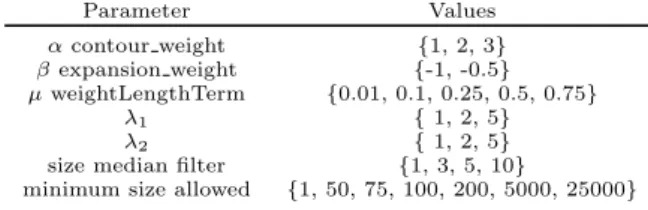
For CV, GAC, DSGAC and DSCV, all the possible combinations of the values in Table 1 were tested. Also, a pre-processing and a post-processing stages were included to improve the results obtained. The post-processing stage
makes a refinement of the results removing the connected components smaller than a certain amount of pixels, while the pre-processing is a median filter to remove salt-and-pepper-like noise present in some of the images. More-over, for DSGAC and DSCV, 10 different initial masks were created using DS and the best one was used in the tuning. The number of iterations for GAC and CV was set to 500 to ensure the process reached convergence. In a few cases, on the ISH dataset, CV failed to converge within the limit due to poor parameters values. This oc-curred only while producing very low quality, degenerate segmentations, therefore the early stopping did not affect the tuning process.
After tuning these methods, the minimum allowed size in pixels of connected components was set to 75, 200 and 25000 for MRI, CT and ISH, respectively. For ASM+RF, the parameters used (Table 3) were those suggested in the bibliography for the ISH dataset, which has been deeply tested by the authors.
For HybridLS, the parameters settings were learned by the GA using the training data. The size of the population was set to 50 individuals, and the evolution lasted 50 gen-erations. The probability of crossover and mutation was set to 0.7 and 0.1, respectively, and the size of the tourna-ment was 3. The range of λ1, λ2was restricted to {1, 2, 5}
to match the settings used with the other methods. The final parameters configurations are reported in Ta-ble 2. It is interesting to remark how the GA detected a different level of importance for each term across the datasets. For instance, in MRI the edge term is not used (we = 0) since our machine learning system determines
that, for a good segmentation, the region term and prior shape knowledge are enough. When segmenting CT lungs the only term used is the region-based one. In this case, λ1
and λ2were set to 5 and 2, respectively. This means that
our final segmentation will have a more uniform foreground region (since the energy contributed by the “variance” in the foreground region has a larger weight), at the expense of allowing more variation in the background.
Table 1: Combination of parameters tested for CV, GAC, DSCV and DSGAC. Parameter Values α contour weight {1, 2, 3} β expansion weight {-1, -0.5} µ weightLengthTerm {0.01, 0.1, 0.25, 0.5, 0.75} λ1 { 1, 2, 5} λ2 { 1, 2, 5} size median filter {1, 3, 5, 10}
minimum size allowed {1, 50, 75, 100, 200, 5000, 25000}
4.4. Experimental results
To evaluate the performance of the segmentation meth-ods, we employed three standard segmentation metrics: the Dice coefficient (DSC), the Jaccard similarity index (JI) and the Hausdorff distance (HD). Both the Dice co-efficient and the Jaccard index measure set agreement: a
Table 2: Parameters obtained after tuning ST, GAC, CV, DS+GAC, DS+CV, and training HybridLS.
CV GAC CV+DS GAC+DS HybridLS Magnetic Resonance Imaging
500 iterations 500 iterations 500 iterations 500 iterations λ1= 5 ν = 0 β = -1 ν = 0 β = -0.5 λ2= 1 µ = 0.01 α = 3 µ = 0.01 α = 3 wr= 5.1 λ1= λ2= 1 medFiltSize = 3 λ1= 1 medFiltSize = 1 wp= 1.1 medFiltSize = 1 λ2=1 we= 0
medFiltSize = 5 γ = 1.5
Computerized Tomography - Knee
500 iterations 500 iterations 500 iterations 500 iterations λ1= 2 ν = 0 α = 1 ν = 0 α = 3 λ2= 5 µ = 0.01 β = -0.5 µ = 0.01 β = -0.5 wr= 4.8 λ1= 5 medFiltSize = 1 λ1= 1 medFiltSize = 1 wp= 0.9
λ2= 2 λ2= 1 we= 2
medFiltSize = 3 medFiltSize = 1 γ = 1.5
Computerized Tomography - Lungs
500 iterations 500 iterations 500 iterations 500 iterations λ1= 5 ν = 0 β = -1 ν = 0 β = -1 λ2= 2 µ = 0.01 α = 2 µ = 0.01 α = 3 wr= 1.5 λ1= 5 medFiltSize = 3 λ1=1 medFiltSize = 3 wp= 0
λ2= 2 λ2= 5 we= 0
medFiltSize = 3 medFiltSize = 3 γ = 1.5
In Situ Hybridization-derived images
500 iterations 500 iterations 500 iterations 500 iterations λ1= 1 ν = 0 β = -1 ν = 0 β = -1 λ2= 1 µ = 0.01 α = 3 µ = 0.01 α = 3 wr= 1.9 λ1= λ2= 1 medFiltSize = 10 λ1= 1 medFiltSize = 10 wp= 2.2 medFiltSize = 5 λ2= 1 we= 1
medFiltSize = 5 γ = 2
Table 3: Parameters used in ST, DS and ASM+RF. All parameters were taken from the original proposals.
ST ASM+RF DS
L = 2 regions Cr = 0.9 Metric = AdvancedNormalizedCorrelation Relative max F = 0.7 Optimizer = ScatterSearch
normalization Uniform Crossover SSb= 12 DE/target-to-best/1 PSize = 32 Population Size = 80 BLX-α = 0.3 Iterations = 250 LS-iterations = 25 Median Filter [25×25] NumberOfIterations = 15 RF with 500 trees NumberOfResolutions = 3
NumberOfSpatialSamples = 2000 5000 10000 Restarts = 3
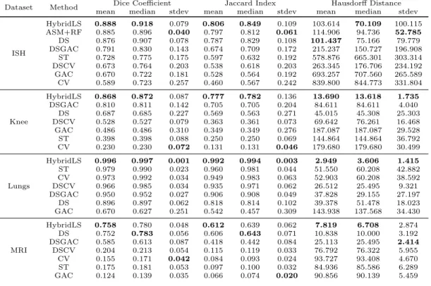
value of 0 indicates no overlap with the ground truth, and a value of 1 indicates perfect agreement. In turn, the Haus-dorff distance measures the mutual proximity of two im-ages, calculated as the maximum distance from a point in the ground truth to the closest point in the segmentation. It is important to remark that ASM+RF, DS, DSCV, DSGAC and HybridLS are non-deterministic, since stochas-tic methods, like Differential Evolution or Scatter Search, are embedded in these algorithms. It is essential to exe-cute such algorithms several times to estimate and com-pare their performances. In this case, 20 repetitions per image were run and the mean, median and standard devi-ation values were calculated over the whole set of results (see Table 5). For instance, in ISH the mean Dice value of DS is 0.876, and represents the average of 440 experiments performed (20 repetitions per image and 22 images).
We also performed a statistical analysis of the results. When comparing two methods, we used Wilcoxon rank-sum test [58], a non-parametric statistical test that checks whether one of two independent samples tends to have larger values than the other. When multiple comparisons were performed, Holm correction [59] was applied to the p-values to control the family-wise error rate. Note that, in the Lungs and Knee datasets, the number of images is not large enough to allow the comparison of the deterministic methods (ST, CV and GAC), therefore they have been excluded from the test.
In Table 4, some concise information about the running time of each algorithm is provided with an illustrative pur-pose. The fastest method is ST with MRI, taking only 1 second per image, while the slowest are the different ap-plications of DS to ISH, employing up to 10 minutes to process an image. Nevertheless, several factors affect the accuracy of a comparison in terms of execution time. First, some of the methods have been developed in MATLAB and others in C++. Moreover, the size of the images dif-fers from one image modality to another, as well as some of the pre- and post-processing stages we used. Finally, the nature of the algorithms is completely different, making them hardly comparable.
4.4.1. Analysis
The experimental results are reported in Table 5. Vi-sual examples of two segmentations obtained by the meth-ods on each dataset are provided in Figure 6. For simplic-ity, our discussion focuses on the results in terms of mean DSC, but note that this choice does not really affect the outcome of the comparison, as there is an almost perfect agreement with the other validation measures we consid-ered.
The performance of the segmentation methods varies greatly across the four datasets. The easiest problem to be solved has been the segmentation of Lungs in CT images, with all methods but GAC and DS scoring higher than 0.95. The most complex task has shown to be the segmen-tation of deep anatomical structures in brain MRI, where
four of the compared methods have obtained an average DSC of 0.2 or less).
The per-dataset results are shown in Figure 5 using boxplots and in Table 6 through the average rankings. Ob-viously, the performance of every method depends on the nature of the image to be segmented. For instance, tech-niques based on grey intensity level (such as CV and ST) yielded worse results in image modalities with less contrast and small differences in terms of pixel intensity like MRI. HybridLS has obtained the best results in all biomed-ical image datasets. It achieved the best values for the mean DSC and JI metrics, and it was ranked as the best method in every image modality. The Wilcoxon test (Ta-ble 6) showed, with really high confidence, that the differ-ence between HybridLS and the other methods is statis-tically significant in all but one case (DS on MRI). This behavior is also robust, as shown by the low standard de-viation values. We can then conclude that our proposal is the best segmentation method in the comparison.
The DS method has been one of the best-performing algorithms, ranking second or third over three datasets. More in general, all methods using the registration-based initialization scored better than those using a standard one. This applies also to CV and GAC: in all but one case, both DSCV and DSGAC ranked better than their counterpart, with a statistically significant difference (Ta-ble 7).
Overall, DSGAC delivered an acceptable performance, ranking above average in three datasets out of four. This is remarkable, as the regular GAC ranked constantly in the last three positions, and it can be explained by the high sensitivity of GAC to its initialization.
DSCV ranked around average in all datasets, perform-ing slightly worse, although more consistently, than DSGAC. The plain CV method achieved a bad performance, rank-ing last or second to last in three datasets. Only on the Lungs dataset, where the grey value is enough to segment the target quite accurately, CV delivered good results.
ST results showed a similar pattern to CV. It per-formed better than CV, but being ST based on the his-togram it showed limited ability to cope with complex scenarios. On the other hand, ST is the fastest method on the group and it has virtually no parameters to be set. ASM+RF obtained some of the best results with ISH images, being also one of the fastest techniques, but it is fair to underline its ad-hoc nature. It needs a training set of shapes to create the template and its possible deforma-tions, and it also needs a training set of textural patterns for the expansion phase. Also, it is not able to manage topological changes in a natural way, as geometric DMs can do.
Finally, from the values of HD, it is interesting to no-tice how methods without shape deformation restrictions, like ST, CV and GAC, have a higher (worse) HD with respect to others introducing prior shape knowledge, like ASM+RF, DS and HybridLS.
Table 4: Average execution time per method and kind of image. All values are in seconds, and were obtained running the experiments in an Intel Core i5-2410M @ 2.3GHz with 4.00 GB of RAM. Also the programming environment has been included between brackets.
ASM+RF ST CV GAC DSCV DSGAC DS HybridLS
(MATLAB, C++) (MATLAB) (MATLAB) (MATLAB, C++) (MATLAB, C++) (MATLAB, C++) (C++) (C++)
ISH 35 39 87 32 582 493 471 545
Lungs - 1.7 36 15 384 342 326 331
Knee - 2.5 67 16 310 265 245 252
MRI - 1 11 1.5 429 407 404 405
Table 5: Segmentation Results using 3 different metrics: Dice Similarity Coefficient (DSC), Jaccard Index (JI), and Hausdorff Distance (HD). Values are sorted in descending order using as criterion their average DSC value. The best results for every metric are shown in bold letters.
Dataset Method Dice Coefficient Jaccard Index Hausdorff Distance mean median stdev mean median stdev mean median stdev
ISH HybridLS 0.888 0.918 0.079 0.806 0.849 0.109 103.614 70.109 100.115 ASM+RF 0.885 0.896 0.040 0.797 0.812 0.061 114.906 94.736 52.785 DS 0.876 0.907 0.078 0.787 0.829 0.108 101.437 75.166 79.779 DSGAC 0.791 0.830 0.143 0.674 0.709 0.172 215.237 150.727 196.908 ST 0.728 0.775 0.175 0.597 0.632 0.192 578.876 665.301 303.314 DSCV 0.673 0.764 0.203 0.538 0.618 0.203 263.345 176.706 234.192 GAC 0.670 0.722 0.181 0.528 0.564 0.192 693.257 707.560 265.589 CV 0.589 0.723 0.257 0.460 0.567 0.242 839.800 844.773 331.804 Knee HybridLS 0.868 0.872 0.087 0.777 0.782 0.136 13.690 13.618 1.735 DSGAC 0.810 0.811 0.142 0.705 0.705 0.204 84.611 84.611 4.040 DS 0.687 0.685 0.227 0.569 0.563 0.271 45.015 45.308 25.303 DSCV 0.528 0.527 0.079 0.363 0.361 0.073 69.642 76.261 16.468 GAC 0.486 0.486 0.310 0.349 0.349 0.276 187.087 187.087 29.528 ST 0.398 0.398 0.088 0.250 0.250 0.069 144.864 144.864 36.792 CV 0.230 0.230 0.072 0.131 0.131 0.046 179.680 179.680 30.499 Lungs HybridLS 0.996 0.997 0.001 0.992 0.994 0.003 2.949 3.606 1.415 ST 0.979 0.990 0.023 0.960 0.981 0.044 51.550 60.208 42.882 CV 0.973 0.992 0.034 0.949 0.983 0.063 52.903 60.208 38.592 DSCV 0.966 0.985 0.034 0.935 0.971 0.062 26.512 25.495 9.321 DSGAC 0.950 0.952 0.027 0.906 0.908 0.049 37.828 29.155 27.197 DS 0.896 0.897 0.062 0.818 0.814 0.102 39.378 51.478 18.023 GAC 0.670 0.627 0.251 0.542 0.457 0.309 143.938 137.568 34.430 MRI HybridLS 0.758 0.780 0.048 0.612 0.639 0.062 7.819 6.708 2.874 DS 0.752 0.783 0.056 0.606 0.643 0.071 10.838 10.000 3.192 DSGAC 0.585 0.613 0.087 0.418 0.442 0.084 25.113 25.495 2.414 DSCV 0.204 0.213 0.054 0.115 0.119 0.033 76.792 76.322 5.955 CV 0.155 0.171 0.042 0.084 0.093 0.024 93.727 93.408 4.670 ST 0.175 0.181 0.053 0.097 0.100 0.032 84.936 85.586 6.289 GAC 0.124 0.139 0.035 0.066 0.074 0.020 90.856 90.139 5.459
original image ST CV GAC DSCV DSGAC DS HybridLS ASM+RF Figure 6: Some visual examples of the results obtained. Two images per image modality and structure to segment have been selected: the first two rows correspond to ISH, the next two rows to CT-Knee, and the last four to CT-Lungs and MRI. White represents true positives, red false negatives, and green false positives.
Table 6: Average rank achieved by every method per im-age modality and adjusted p-value of Wilcoxon test com-paring each algorithm against HybridLS.
Dataset Method Mean Rank p-value
ISH HybridLS 1.82 DS 2.50 0.000 ASM+RF 2.64 0.000 DSGAC 4.14 0.000 ST 5.68 0.000 DSCV 6.23 0.000 GAC 6.36 0.000 CV 6.64 0.000 Knee HybridLS 1.50 DSGAC 2.00 0.000 DS 3.00 0.000 DSCV 4.50 0.000 GAC 5.00 -ST 5.50 -CV 6.50 -Lungs HybridLS 1.00 ST 2.33 -CV 3.00 -DSCV 3.67 0.000 DSGAC 5.33 0.000 DS 5.67 0.000 GAC 7.00 -MRI HybridLS 1.27 DS 1.73 0.46 DSGAC 3.00 0.000 DSCV 4.18 0.000 ST 5.09 0.000 CV 5.73 0.000 GAC 7.00 0.000
Table 7: Pairwise comparison of all the methods but HybridLS. Each cell of the table reports the p-value of Wilcoxon test comparing the method on the correspond-ing row with that on the column.
ISH
ASM+RF CV DS DSCV DSGAC GAC CV 0.00 DS 0.01 0.00 DSCV 0.00 0.38 0.00 DSGAC 0.00 0.00 0.00 0.00 GAC 0.00 0.92 0.00 0.92 0.00 ST 0.00 0.32 0.00 0.61 0.26 0.61 Knee DS DSCV DSCV 0.00 DSGAC 0.00 0.00 Lungs DS DSCV DSCV 0.00 DSGAC 0.00 0.00 MRI CV DS DSCV DSGAC GAC DS 0.00 DSCV 0.02 0.00 DSGAC 0.00 0.00 0.00 GAC 0.10 0.00 0.00 0.00 ST 0.79 0.00 0.26 0.00 0.08 0.0 0.2 0.4 0.6 0.8 1.0 ST HybridLS GAC DSGAC DSCV DS CV ASM+RF ISH 0.0 0.2 0.4 0.6 0.8 1.0 ST HybridLS GAC DSGAC DSCV DS CV Knee 0.0 0.2 0.4 0.6 0.8 1.0 ST HybridLS GAC DSGAC DSCV DS CV Lungs 0.0 0.2 0.4 0.6 0.8 1.0 ST HybridLS GAC DSGAC DSCV DS CV MRI
5. Discussion and Future Research
It is crucial to highlight the main features of HybridLS: • it is an accurate and also general segmentation method
(it obtains very good results with all the medical im-age modalities tested, even overcoming well-consolidated techniques);
• its overall standard deviation is the lowest among the different methods compared, therefore we can affirm that the developed approach is consistent and stable in terms of performance;
• it does not need a training set of textures or shapes to segment the object of interest (it needs only one reference image to obtain the shape prior);
• it performs self-adaptation of its own parameters de-pending on the medical image modality to segment; • and uses metaheuristics to generate the shape prior and to perform the previously mentioned learning of parameters.
Thanks to the automatic learning of the model param-eters, our hybrid proposal is able to perform an effective segmentation with very different medical image modali-ties, adapting the importance of every term to each image modality and anatomical structure.
The main drawback of HybridLS is that it is not as fast as ST or even ASM+RF. This is obvious since it can be as fast as its components and, evidently, DS is a de-formable registration process that can take several minutes in a general purpose computer. More sophisticated imple-mentations, like GPGPU programming, can be tested to speed-up the computations. Finally, the introduction of a textural term could be taken into consideration if the benefits obtained with its use justify it.
Acknowledgments
Pablo Mesejo and Andrea Valsecchi are funded by the European Commission (Marie Curie ITN MIBISOC, FP7 PEOPLE-ITN-2008, GA n. 238819). The authors want to thank Nicola Bova for his generous and helpful advice on the development of the level set implementation. NMR database is the property of “CEA/I2BM/NeuroSpin” and can be provided on demand to [email protected]. Data were acquired with PTK pulse sequences, reconstructed with PTK reconstructor package and postprocessed with Brainvisa/Connectomist software, freely available at http: //brainvisa.info.
References
[1] D. L. Pham, C. Xu, J. L. Prince, Current Methods in Medical Image Segmentation, Annual Review of Biomedical Engineering 2 (2000) 315–337.
[2] L. He, Z. Peng, B. Everding, X. Wang, C. Y. Han, K. L. Weiss, W. G. Wee, A comparative study of deformable contour meth-ods on medical image segmentation, Image and Vision Comput-ing 26 (2008) 141–163.
[3] T. Heimann, H.-P. Meinzer, Statistical shape models for 3D medical image segmentation: a review, Medical Image Analysis 13 (2009) 543–563.
[4] J. Malik, S. Belongie, T. Leung, J. Shi, Contour and Texture Analysis for Image Segmentation, International Journal of Com-puter Vision 43 (1) (2001) 7–27, ISSN 0920-5691.
[5] Y. Zhang, B. J. Matuszewski, L.-K. Shark, C. J. Moore, Medi-cal Image Segmentation Using New Hybrid Level-Set Method, in: Procs. of the International Conference BioMedical Visual-ization: Information Visualization in Medical and Biomedical Informatics, 71–76, 2008.
[6] M. Chupin, A. Hammers, R. S. N. Liu, O. Colliot, J. Burdett, E. Bardinet, J. S. Duncan, L. Garnero, L. Lemieux, Automatic segmentation of the hippocampus and the amygdala driven by hybrid constraints: Method and validation, NeuroImage 46 (3) (2009) 749–761.
[7] M. Gendreau, J.-Y. Potvin, Handbook of Metaheuristics, Springer Publishing Company, Incorporated, 2nd edn., ISBN 1441916636, 9781441916631, 2010.
[8] D. E. Goldberg, Genetic Algorithms in Search, Optimization and Machine Learning, Addison-Wesley, 1989.
[9] M. Laguna, R. Mart´ı, Scatter search: methodology and imple-mentations in C, Kluwer Academic Publishers, Boston, 2003. [10] D. Terzopoulos, K. Fleischer, Deformable Models, The Visual
Computer 4 (1988) 306–331.
[11] M. Kass, A. Witkin, D. Terzopoulos, Snakes: Active contour models, International Journal of Computer Vision 1 (1988) 321– 331.
[12] T. F. Cootes, C. J. Taylor, D. H. Cooper, J. Graham, Active shape models-their training and application, Computer Vision and Image Understanding 61 (1995) 38–59.
[13] T. F. Cootes, G. J. Edwards, C. J. Taylor, Active Appearance Models, in: Proc. of the European Conference on Computer Vision, vol. 2, 484–498, 1998.
[14] T. F. Cootes, G. Edwards, C. Taylor, Comparing Active Shape Models with Active Appearance Models, in: Procs. of British Machine Vision Conference, 173–182, 1999.
[15] M. Bro-Nielsen, Active nets and cubes, Tech. Rep., 1994. [16] B. B. Kimia, A. R. Tannenbaum, S. W. Zucker, Shapes, Shocks,
and Deformations I: The Components of Two-Dimensional Shape and the Reaction-Diffusion Space, International Journal of Computer Vision 15 (1994) 189–224.
[17] R. Kimmel, A. Amir, A. M. Bruckstein, Finding Shortest Paths on Surfaces Using Level Sets Propagation, IEEE Trans. on Pat-tern Analysis and Machine Intelligence 17 (6) (1995) 635–640. [18] G. Sapiro, A. Tannenbaum, Affine Invariant Scale-Space,
Inter-national Journal of Computer Vision 11 (1) (1993) 25–44. [19] S. Osher, J. Sethian, Fronts propagating with
curvature-dependent speed: algorithms based on Hamilton-Jacobi formu-lations, Journal of Computational Physics 79 (1) (1988) 12–49. [20] J. Sethian, Level Set Methods and Fast Marching Methods: Evolving Interfaces in Computational Geometry, Fluid Mechan-ics, Computer Vision, and Materials Science, Cambridge Mono-graphs on Applied and Computational Mathematics, Cam-bridge University Press, 1999.
[21] S. J. Osher, R. P. Fedkiw, Level Set Methods and Dynamic Implicit Surfaces, Springer, 2002.
[22] S. Luke, Essentials of Metaheuristics, Lulu, available for free at http://cs.gmu.edu/∼sean/book/metaheuristics/, 2009. [23] B. Zitov´a, J. Flusser, Image registration methods: a survey,
Image and Vision Computing 21 (2003) 977–1000.
[24] J. P. W. Pluim, J. B. A. Maintz, M. A. Viergever, Mutual-information-based registration of medical images: a survey, IEEE T. Med. Imaging 22 (8) (2003) 986–1004.
[25] F. Maes, D. Vandermeulen, P. Suetens, Comparative evaluation of multiresolution optimization strategies for image registration by maximization of mutual information, Medical Image
Analy-sis 3 (4) (1999) 373–386.
[26] S. Klein, M. Staring, J. P. W. Pluim, Evaluation of Optimiza-tion Methods for Nonrigid Medical Image RegistraOptimiza-tion Using Mutual Information and B-Splines, IEEE Trans. on Image Pro-cessing 16 (12) (2007) 2879–2890.
[27] S. Damas, O. Cord´on, J. Santamar´ıa, Medical Image Registra-tion Using EvoluRegistra-tionary ComputaRegistra-tion: An Experimental Sur-vey, IEEE Computational Intelligence Magazine 6 (4) (2011) 26 –42.
[28] M. Cabezas, A. Oliver, X. Llad´o, J. Freixenet, M. B. Cuadra, A review of atlas-based segmentation for magnetic resonance brain images, Computer Methods and Programs in Biomedicine 104 (3) (2011) e158 – e177.
[29] P. Mesejo, R. Ugolotti, F. D. Cunto, M. Giacobini, S. Cagnoni, Automatic Hippocampus Localization in Histological Images using Differential Evolution-Based Deformable Models, Pattern Recognition Letters 34 (3) (2013) 299 – 307.
[30] M. Heydarian, M. Noseworthy, M. Kamath, C. Boylan, W. Poehlman, Optimizing the Level Set Algorithm for Detect-ing Object Edges in MR and CT Images, IEEE Trans. on Nu-clear Science 56 (1) (2009) 156 –166.
[31] L. Ballerini, Genetic Snakes for Medical Images Segmenta-tion, in: Evolutionary Image Analysis, Signal Processing and Telecommunications, vol. 1596, 59–73, 1999.
[32] D.-H. Chen, Y.-N. Sun, A self-learning segmentation frame-work—the Taguchi approach, Computerized Medical Imaging and Graphics 24 (5) (2000) 283 – 296.
[33] C. McIntosh, G. Hamarneh, Medial-based Deformable Models in Non-convex Shape-spaces for Medical Image Segmentation using Genetic Algorithms, IEEE Trans. on Medical Imaging 31 (1) (2012) 33–50.
[34] C.-Y. Hsu, C.-Y. Liu, C.-M. Chen, Automatic segmentation of liver PET images, Computerized Medical Imaging and Graphics 32 (7) (2008) 601 – 610.
[35] O. Ib´a˜nez, N. Barreira, J. Santos, M. G. Penedo, Genetic approaches for topological active nets optimization, Pattern Recognition 42 (5) (2009) 907–917.
[36] J. Novo, J. Santos, M. G. Penedo, Topological Active Models optimization with Differential Evolution, Expert Systems with Applications 39 (15) (2012) 12165–12176.
[37] N. Bova, ´O. Ib´a˜nez, O. Cord´on, Image Segmentation Using Ex-tended Topological Active Nets Optimized by Scatter Search, IEEE Computational Intelligence Magazine 8 (1) (2013) 16–32. [38] P. Ghosh, M. Mitchell, J. A. Tanyi, A. Hung, A Genetic Algorithm-Based Level Set Curve Evolution for Prostate Seg-mentation on Pelvic CT and MRI Images, in: Biomedical Image Analysis and Machine Learning Technologies, 127–149, 2010. [39] D. Feltell, L. Bai, 3D level set image segmentation refined by
intelligent agent swarm, in: Procs. of IEEE Congress on Evolu-tionary Computation, 1–8, 2010.
[40] P. Mesejo, S. Cagnoni, An experimental study on the automatic segmentation of in situ hybridization-derived images, in: Proc. on 1st International Conference on Medical Imaging using Bio-Inspired and Soft Computing (MIBISOC’13), in Press, 2013. [41] A. Valsecchi, S. Damas, J. Santamar´ıa, L. Marrakchi-Kacem,
Intensity-based Image Registration using Scatter Search, Tech. Rep. AFE 2012-14, URL http://docs.softcomputing.es/ public/afe/TR-AFE-2012-14.pdf, submitted to Artificial Intel-ligence in Medicine, 2012.
[42] O. Cord´on, S. Damas, J. Santamar´ıa, R. Mart´ı, Scatter Search for the Point-Matching Problem in 3D Image Registration, IN-FORMS Journal on Computing 20 (1) (2008) 55–68.
[43] T. F. Chan, L. A. Vese, Active Contours without Edges, IEEE Trans. on Image Processing 10 (2001) 266–277.
[44] B. Li, S. Member, S. T. Acton, S. Member, Active contour exter-nal force using vector field convolution for image segmentation, IEEE Trans. on Image Processing 16 (2007) 2096–2106. [45] C. Xu, J. L. Prince, Gradient Vector Flow: A New External
Force for Snakes, in: Procs. of IEEE Conference on Computer Vision and Pattern Recognition, 66–71, 1997.
[46] R. C. Gonzalez, R. E. Woods, Digital Image Processing,
Addison-Wesley, 2nd edn., 2001.
[47] Y. Shi, W. C. Karl, A Real-Time Algorithm for the Approx-imation of Level-Set-Based Curve Evolution, IEEE Trans. on Image Processing 17 (5) (2008) 645–656.
[48] L. J. Eshelman, J. D. Schaffer, Real-coded genetic algorithms and interval-schemata., in: D. L. Whitley (Ed.), Foundation of Genetic Algorithms 2, Morgan Kaufmann., San Mateo, CA, 187–202, 1993.
[49] T. B¨ack, D. B. Fogel, Z. Michalewicz, Handbook of Evolutionary Computation, IOP Publishing Ltd and Oxford University Press, 1997.
[50] Allen Institute for Brain Science, Allen Reference Atlases, http: //mouse.brain-map.org, 2004-2006.
[51] C. Poupon, F. Poupon, L. Allirol, J.-F. Mangin, A database dedicated to anatomo-functional study of human brain connec-tivity, in: Procs. of the Annual Meeting of the Organization for Human Brain Mapping, 646, 2006.
[52] P. Mesejo, R. Ugolotti, S. Cagnoni, F. Di Cunto, M. Giacobini, Automatic Segmentation of Hippocampus in Histological Im-ages of Mouse Brains using Deformable Models and Random Forest, in: Procs. of Symposium on Computer-Based Medical Systems, 2012.
[53] S. Das, P. Suganthan, Differential Evolution: A Survey of the State-of-the-Art, IEEE Trans. on Evolutionary Computation 15 (2011) 4–31.
[54] N. Otsu, A Threshold Selection Method from Gray-Level His-tograms, IEEE Trans. on Systems, Man and Cybernetics 9 (1) (1979) 62 –66.
[55] L. Breiman, Random Forests, Maching Learning 45 (2001) 5–32. [56] S. Aja-Fernandez, G. Vegas-Sanchez-Ferrero, M. Martin Fer-nandez, Soft thresholding for medical image segmentation, in: Proc. International Conference of the IEEE Engineering in Medicine and Biology Society (EMBC), 4752 –4755, 2010. [57] V. Caselles, R. Kimmel, G. Sapiro, Geodesic Active Contours,
International Journal of Computer Vision 22 (1997) 61–79. [58] W. H. Kruskal, Historical Notes on the Wilcoxon Unpaired
Two-Sample Test, Journal of the American Statistical Association 52 (279) (1957) 356–360.
[59] S. Holm, A Simple Sequentially Rejective Multiple Test Proce-dure, Scandinavian Journal of Statistics 6 (2) (1979) 65–70.