HAL Id: hal-02044488
https://hal.archives-ouvertes.fr/hal-02044488v3
Submitted on 18 Feb 2019
HAL is a multi-disciplinary open access
archive for the deposit and dissemination of
sci-entific research documents, whether they are
pub-lished or not. The documents may come from
teaching and research institutions in France or
abroad, or from public or private research centers.
L’archive ouverte pluridisciplinaire HAL, est
destinée au dépôt et à la diffusion de documents
scientifiques de niveau recherche, publiés ou non,
émanant des établissements d’enseignement et de
recherche français ou étrangers, des laboratoires
publics ou privés.
Pierre Brisset, Jerome Monnier, Pierre-André Garambois, Hélène Roux
To cite this version:
Pierre Brisset, Jerome Monnier, Pierre-André Garambois, Hélène Roux. On the assimilation of
alti-metric data in 1D Saint-Venant river flow models. Advances in Water Resources, Elsevier, 2018, 119,
pp.41-59. �10.1016/j.advwatres.2018.06.004�. �hal-02044488v3�
PIERRE BRISSET (1)(2), JÉRÔME MONNIER * (1)(2), PIERRE-ANDRÉ GARAMBOIS (3)(4), HÉLÈNE ROUX (5)(6)
3
(1) Institut de Mathématiques de Toulouse (IMT), Toulouse, France.
4
(2) INSA Toulouse, France.
5
(3) INSA Strasbourg, France.
6
(4) ICUBE, Strasbourg, France.
7
(5) INPT Toulouse, France.
8
(6) Institut de Mécanique des Fluides (IMFT), Toulouse, France.
9 10
* Corresponding author: jerome.monnier@insa-toulouse.fr
11 12
Abstract. Given altimetry measurements, the identification capability of time varying inflow discharge Qin(t) and 13
the Strickler coefficient K (defined as a power-law in h the water depth) of the 1D river Saint-Venant model is
investi-14
gated. Various altimetry satellite missions provide water level elevation measurements of wide rivers, in particular the
15
future Surface Water and Ocean Topography (SWOT) mission. An original and synthetic reading of all the available
16
information (data, wave propagation and the Manning-Strickler’s law residual) are represented on the so-called
iden-17
tifiability map. The latter provides in the space-time plane a comprehensive overview of the inverse problem features.
18
Inferences based on Variational Data Assimilation (VDA) are investigated at the limit of the data-model inversion
19
capability : relatively short river portions, relatively infrequent observations, that is inverse problems presenting a
20
low identifiability index. The inflow discharge Qin(t)is infered simultaneously with the varying coefficient K(h). The 21
bed level is either given or infered from a lower complexity model. The experiments and analysis are conducted for
22
different scenarios (SWOT-like or multi-sensors-like). The scenarios differ by the observation frequency and by the
23
identifiability index. Sensitivity analyses with respect to the observation errors and to the first guess values
demon-24
strate the robustness of the VDA inferences. Finally this study aiming at fusing relatively sparse altimetric data and
25
the 1D Saint-Venant river flow model highlights the spatiotemporal resolution lower limit, also the great potential in
26
terms of discharge inference including for a single river reach.
27 28
Keywords. River flow, variational data assimilation, altimetry, SWOT, discharge, Saint-Venant, Manning,
Strick-29
ler.
30
1. Introduction
31
While the in situ observation of the continental water cycle, especially river flows, is declining, satellites provide
32
increasingly accurate measurements. The future Surface Water and Ocean Topography (SWOT) mission
(CNES-33
NASA, planned to be launched in 2021) equipped with a swath mapping radar interferometer will provide river
34
surface mapping at a global scale with an unprecedented spatial and temporal resolution - decimetric accuracy on
35
water surface height averaged over 1 km² [46]. An other highlight of SWOT will be its global coverage and temporal
36
revisits (1 to 4 revisits per 21-days repeat cycle). In complementarity with decades of nadir altimetry on inland
37
waters [7], SWOT should offer the opportunity to increase our knowledge of the spatial and temporal distribution of
38
hydrological fluxes including stream and rivers see e.g. [3, 4]. Thanks to this increased observation of water surfaces
39
worldwide, it will be possible to address a variety of inverse problems in surface hydrology and related fields, see e.g.
40
[43]. Given these surface measurements (elevation, water mask extents), the challenging inverse problems consist to
41
infer the discharge but also the unobservable cross sections, the roughness coefficients and the lateral contributions.
42
These inverse problems are more or less challenging depending on the space-time observations density, the targeted
43
space-time resolution, the potential prior information and the measurements errors.
44
A relatively recent literature addresses some of these inverse questions including in a pure remote sensing data
45
context potentially sparse both in space and time, see e.g. [4] for a recent review. Few low-complexity methods, based
46
either on steady-state flow models (like the Manning-Strikler’s law) or hydraulic geometries (empirical power-laws)
47
have been developed, see [5, 16, 18, 56]. In [15] the performances obtained on 19 rivers with artificially densified daily
48
observables are fluctuating depending on the algorithm tested. In order to better constrain these under-determined
49
inverse problems, prior hydraulic information or empirical laws may be required. It is shown in [18] with a steady
50
model that given one (1) bed level measurement, an effective bathymetry can be infered quite accurately throughout
51
the river reach; see also [21, 22] in a purely academic context. No approach aforementioned does satisfactorily solve
52
the equifinality issue related to the bathymetry and friction. Indeed if infering the triplet formed by the bathymetry,
53
friction and discharge then an equifinality issue is a-priori encountered, see e.g. the discussion led in [18].
54 55
In the river hydraulic community, the most employed data assimilation studies are based on sequential algorithms,
56
the Kalman filter and its variants. Let us cite for example [8, 47, 48] who estimate flood hydrographs in the 1D
Saint-57
Venant model from dense water surface width measurements; the bathymetry and roughness are given. [45] considers
58
a diffusive wave model with the bathymetry and friction coefficients given; it corrects the upstream discharge via
59
the assimilation of downstream water depth measurements. The persistence in time of the correction due to the
60
assimilation of synthetic SWOT observations on discharge forecasts of ⇠ 500 km of the Ohio river is assessed by [1].
61
[40] shows the benefit of assimilating virtual SWOT observations for optimizing Selingue dam release (lake depth) and
62
river depth in the upper Niger basin. The impact of the hydraulic propagation time (25 days at low flow) compared to
63
synthetic SWOT observation maximum spacing (9 days in this case) on assimilation methods is highlighted through
64
downstream discharge estimates. Most of those twin experiments use temporal observation sampling much greater
65
than the hydrodynamic phenomena time scales, moreover in large river reaches (potentially in network) of several
66
hundreds of km. This ensures multiple measurements of the flow variations. The infered parameters are generally the
67
water depth h or a constant Strickler coefficient K but rarely both parameters simultaneously.
68 69
Despite the huge improvement of the remotely sensed data (e.g. by satellite altimetry) and the use of data
assimila-70
tion methods (variational or sequential), the relative sparsity of the acquired data is challenging for river applications.
71
If considering a “small scale” river portion regarding satellite spatio-temporal sampling, typically hundred
kilome-72
ters long, the hydraulic information propagates faster than the satellites revisit. The model inversions are generally
73
performed at observation times and propagated with a Kalman filter see e.g. [55, 40] and [4] for a review.
74
The Variational Data Assimilation (VDA) approach based on the optimal control of the dynamics flow model, see
75
[50, 33, 42, 14] and e.g. [6], consists in minimizing a cost function measuring the discrepancy between the model outputs
76
and the observations. This approach aims at optimally combining somehow in the least square sense, the model, the
77
observations and potential prior statistical information This approach is widely used in meteorology and oceanography
78
since it makes possible to “invert” high-dimensional control vectors and models. In some circumstances, it is possible
79
to infer unknown “input parameters” such as the boundary conditions (e.g. inflow discharge), model parameters (e.g.
80
roughness) and/or forcing terms. Among the first VDA studies related to hydraulic models let us cite [44, 11, 49],
81
next [2, 27, 10] which infer the inflow discharge in 2D shallow water river models. Only a few studies tackle the
82
identification by VDA of the complete unknown set that is the inflow discharge, the roughness and the bathymetry.
83
Infering the discharge and hydraulic parameters from water surface measurements is not straightforward and may
84
be even impossible, depending on the flow regime and the adequacy between the observations density and the flow
85
dynamics. The inference of the triplet (inflow discharge, effective bathymetry and friction coefficient) is investigated
86
in [28, 29] from relatively constraining surface Lagrangian observations. Based on a real river dataset (Pearl river in
87
China), the upstream, downstream and few lateral fluxes are identified from water levels measured at in-situ gauging
88
stations in [27]; however the bathymetry and roughness are given. The assimilation of spatially distributed water
89
level observations in a flood plain (a single image acquired by SAR) and a partial in-situ time series (gauging station)
90
are investigated in [31, 30]. In [20, 34] the inference of inflow discharge and lateral fluxes are identified by VDA by
91
superposing a 2D local “zoom model” over the 1D Saint-Venant model. These studies are not conducted in a sparse
92
altimetry measurement context. More recently [19] have investigated discharge identification of the 1D Saint-Venant
93
model by VDA under uncertainties on the bathymetry and the friction coefficient in a purely academic case.
94
Finally it is worth to mention that the VDA approach provides instructive local analysis sensitivity maps, making
95
possible to better understand the flow and the model, in particular the influence of the bathymetry and local friction
96
coefficient values, see e.g. [37].
97 98
The present study investigates the capabilities of accurate, repetitive but relatively sparse altimetry dataset (SWOT
99
like) to infer time varying river discharges. To do so, firstly the inverse problem is simply represented by the so-called
100
identifiability map. This map represents all the available information in the (x, t) plane, that is the observations (the
101
observed “space-time windows”), the hydrodynamic waves propagation (1D Saint-Venant model) and the misfit to the
102
“local equilibrium” (more precisely the local misfit with the steady state uniform flow represented by the
Manning-103
Strikler law). This preliminary analysis makes possible to roughly estimate the time-windows which can be quantified
104
by VDA since the inflow discharge values arise from these observed “space-time windows”. This original reading of
105
the hydraulic inverse problem is qualitative only but fully instructive. Indeed this makes possible to roughly estimate
106
whether the sought information has been observed or not, in particular in terms of frequency (providing orders of
107
magnitude). Next the inference of the inflow discharge Qin(t)and the Strickler coefficient K, with K depending on the 108
water depth h (that is a power-law depending on the state of the system) is analyses into details. This analysis provides
109
an answer to the temporal variability identifiable given a spatio-temporal distribution of water surface observations.
110
The numerical results are presented first on a so-called “academic” case with synthetic data, making possible to
111
focus on the computational method (based on the classically called twin experiments) without the specific real data
112
difficulties (difficulties due to potential difference of scales, measurement errors, un-modeled subscale phenomena
etc). This case presents a relatively low identifiability index, that is a quite high frequency hydrograph variations
114
compared to the observation frequency. A basic guideline to estimate the a-priori minimal identifiable frequency is
115
provided. Next a river portion (74 km long) of the Garonne river (France) [51, 32] is considered with few scenarios of
116
observation frequency: from the SWOT like data (21 days period with 1 to 4 passes at mid-latitudes) to a
multiple-117
sensor scenario (or SWOT Cal-Val orbit, ⇠ 1 day period). The bathymetry is either provided or estimated from one
118
in-situ measurement following [21, 18]. The computational code developed for the present inverse analyses is part of
119
the computational software DassFlow [36].
120 121 122 123 124 125 126 127 128
The outline of the article is as follows. In Section 2, the 1D Saint-Venant forward model and the inverse method based
129
on VDA are presented, along with the academic test case and the Garonne river case. In Section 3 the identifiability
130
maps are presented and analyses. Next based on the VDA process, the discharge identification is discussed for various
131
observation samplings. In Section 4, numerical experiments are conducted to infer by VDA the pair (Qin(t), K(h)); 132
the bed level is either given or estimated from one (1) in-situ value and a low complexity model. Sensitivities of the
133
infered quantities are analyses with respect to the first guess and the observation errors. In Section 5, the Garonne
134
test case is investigated for two scenarios: the real SWOT temporal sampling (⇠21 days revisiting period) and a data
135
sampling densified by a factor 100 . A conclusion and perspectives are proposed in Section 6. The two appendices
136
present details of the numerical scheme in the present context of altimetry measurements.
137
2. forward-inverse models and test cases
138
In this part, the forward model (1D Saint-Venant equations) and the inverse model, Variational Data Assimilation
139
(VDA), are described. In particular the model geometry (effective river bathymetry), the observation operator and
140
the minimized cost function are detailed.
141
2.1. Forward model. Open channel flows are commonly described with the 1D Saint Venant equations in (S, Q)
142
variables [12, 9]. The model based on the depth-integrated variables is valid under the long-wave assumption
(shallow-143
water). The equations read :
144 (2.1) 8 > < > : @S @t + @Q @x = 0 (2.1.1) @Q @t + @ @x ✓Q2 S + P ◆ = g Z h 0 (h z)@ ˜w @xdz gS[ @zb @x + Sf] (2.1.2) 145
where S is the wet-cross section (m2), Q is the discharge (m3.s 1), P = gRh
0(h z) ˜wdz is the pressure term as 146
proposed in [54], ˜wis the water surface top width (m), g is the gravity magnitude (m.s 2), H is the water surface 147
elevation (m), H = (zb+ h) where zb is the lowest bed level (m) and h is the water depth (m). Sf denotes the basal 148
friction slope (dimensionless) and Sf = |Q|Q K2S2R4/3
h
(classical Manning-Strikler parameterization) with K the Strickler
149
coefficient (m1/3.s 1) and R
h the hydraulic radius (m). The discharge Q is related to the average cross sectional 150
velocity u (m.s 1) by: Q = uS. The left-hand side of the momentum equation is written in its conservative form 151
(hyperbolic part of the model) while the right-hand is a source term. This source term can viewed as pulling the
152
model to the basic equilibrium: the gravitational force vs the friction forces. This classical model is considered with a
153
specific bathymetry geometry built from the water surface observables. The discrete cross sections are asymmetrical
154
trapezium layers; each layer is defined by one triplet (Hi,wi,Yi) corresponding respectively to the water elevation, the 155
water surface width associated to Hi and a centering parameter. In a SWOT context, each layer corresponds to a 156
satellite pass.
157
Remark 1. If the Froude number, F r = u
c, tends towards 0 then the 1D St Venant model can be written as a depth-158
averaged scalar equation: the diffusive wave model, see e.g. [12, 39]. In the case of a wide channel (the hydraulic radius
159
Rh⇡ h), the advective term of the equation corresponds to the velocity 53u. In the identifiability maps presented in 160
a next section, this wave velocity 5
3u is plotted simultaneously with the Saint-Venant model wave velocities, that is 161
(u c) and (u + c) (gravity waves model).
162 163 164
Figure 2.1. Effective geometry considered for each cross section: superimposition of m trapeziums (yz-view).
The Strickler coefficient K is defined as a power law in the water depth h:
165 166
(2.2) K(h) = ↵ h
167
where ↵ and are two constants to be determined. This a-priori law makes possible to set the roughness in function
168
of the flow regime. This power-law is richer than a constant uniform value as it is often set in the literature. Also
169
such a power-law can be defined by sections or reaches.
170
The discharge at upstream boundary Qin(t) will be considered as an unknown variable of the model (it will be a 171
control parameter of the model). It will be defined by one of these two methods:
172
IDbasic.: At each identification time tj, tj 2 [t1..tp], a value of Qin(tj)is computed by the VDA process. Next 173
the identified inflow discharge is continuously constructed by simple linear interpolation.
174
IDFourier.: The inflow discharge is defined as Fourier series:
175 176 (2.3) Qin(t) = a0 2 + NXF S n=1 ✓ ancos(nt 2⇡ T ) + bnsin(nt 2⇡ T ) ◆ 177
where {a0; an, bn}, n 2 [1..NF S], are the Fourier coefficients and T is the total simulation time. The lower frequency 178
represented by the Fourier series is 1/T and the highest one is NF S/T. Then this way to identify Qin(t)is global in 179
time (on the contrary to punctual basic approach above). Obviously, the hydrograph must be periodic. However this
180
is not an issue since the hydrograph can be extended to make a T-periodic function (T denoting the final simulation
181
time).
182
The numerical scheme used is the classical finite volume scheme HLL [25] with Euler integration in time. This
183
numerical scheme with the specificities due to the particular geometrical transformations are presented in Appendix
184
7.1 and Appendix 7.2. The equations above have been implemented into the computational code DassFlow [36]. Note
185
that few numerical schemes are possible: the classical implicit Preissmann’s scheme, the HLL finite volume scheme
186
and also an original semi-implicit multi-regime scheme.
187
2.2. Inverse problem: Variational Data Assimilation (VDA) formulation . The inference of the unknown
188
parameters are performed by the VDA approach. It consists in minimizing a cost function J(k) measuring the
discrep-189
ancy between the model output (state variables) and the available measurements (which are sparse and uncertain):
190
minkJ(k). Since J depends on k through the model solution (S, Q), it is an optimal control problem. It is classi-191
cally solved by introducing the adjoint model and by computing iteratively a “better” control vector k. The latter
192
contains the inflow discharge Qin(t) and the coefficient K(h) defined by (2.2). In the case the unknown parameters 193
are computed at given times [t1..tp](it is the identification time grid), k is defined by: 194
195
k = (Qin,1, ..., Qin,p, ↵, )T 196
In the case the inflow discharge is decomposed as a Fourier series, see 2.3, k is defined by:
197 198
k = (a0, a1, b1..., aNF S, bNF S, ..., ↵, )
T
The VDA process requires the computation of the gradient of the cost function rJ with respect to k. The
200
computation of rJ is done with DassFlow software which has been originally designed to generate automatically the
201
discrete adjoint model using the source to source differentiation tool Tapenade [26]. The cost function expression J
202
depends on the observations; the latter are presented below while the expression of J is detailed in Section 2.5.
203
The employed optimization algorithm is a the L-BFGS algorithm (here the M1QN3 routine [23]). Details on the
204
basis of VDA can be found e.g. in [35]. Given a first guess on parameters k0, the iterates ki are searched with the 205
descent algorithm such as the cost function J decreases. For each iteration of the minimization:
206
(1) The cost function J(ki)and its gradient rJ(ki)are computed by performing the forward model (from 0 to 207
T) and its adjoint (from T to 0).
208
(2) Given ki , J(ki)and rJ(ki), the M1QN3 routine is invoked to compute a new iterate such that: J(ki+1) < 209
J(ki). 210
(3) The few convergence criteria are tested: either |J| 10 7, or |J(k
i+1) J(ki)| 10 5 or i > 100. 211
In order to measure the accuracy of the identified discharge Qident
in = (Qidentin,1 , Qidentin,2 , ..., Qidentin,p )T , the classical Nash-212
Sutcliffe criteria E is considered, [41]:
213 214
(2.4) E(Qidentin ) = 1
Pp
i=1 Qrealin,i Qidentin,i 2
Pp
i=1 Qrealin,i Q¯realin
2 , with ¯Qrealin = p X i=1 Qrealin,i p 215
The vector Qreal
in = (Qrealin,1, Qrealin,2, ..., Qrealin,p)T contains the true values. The Nash-Sutcliffe value E is close to 1 for 216
values of Qident
in close to Qrealin ; it is close to 0 for values of Qidentin close to ¯Qrealin ; finally it is close to 1 for values of 217
Qidentin not correlated to the true value Qrealin . 218
For a given quantity u (it will be Qin, ↵ or ), e2(u) denotes the 2-norm relative error: 219 220 (2.5) e2(u) = ku ident urealk 2 kurealk2 221
2.3. Design of the inversion experiments. The identifiability of the river flow model parameters from water surface
222
observables is studied on a so-called academic test case before being studied on a real data set (a portion of the Garonne
223
river, France). Analyzing an “academic” case first is important to properly analyse the numerical inversions. Indeed,
224
the academic test case makes possible to focus on the computational method (based on the classically called twin
225
experiments) without the specific real data difficulties (difficulties due to potential difference of scales, measurement
226
errors, un-modeled subscale phenomena etc). Then so-called twin experiments are considered. It consist to set the
227
inverse problem as follows:
228
• Realistic true values of the parameters (roughness uniform in space and discharge hydrographs) are fixed.
229
Then the forward model is run, which allows to compute the SWOT like data (that is water elevation H and
230
WS width w at the reach scale -see details in next section-).
231
• Given the perturbed synthetic data, the parameter identifiability is investigated for various temporal samplings
232
of observations. The input “parameters”, inflow discharge Qin(t)and coefficient power-law K(h), are computed 233
by VDA. The inflow discharge may be sought in a reduced Fourier basis; the latter being defined from a-priori
234
fixed frequency. In the first numerical experiments, the bathymetry is given. This makes possible to focus the
235
investigation on the identifiability of the inflow discharge in terms of frequency ratio between the observation
236
and the minimal identified frequency. In the last experiment (Garonne river), the considered bed level can be
237
given or estimated from one in-situ value and following the method presented in [18].
238
2.3.1. Academic test case. The aim of this test case is to investigate the identifiability of several discharge hydrographs
239
and roughness on a fully controlled and low CPU time test case Its geometry consists in a 1000 m length channel.
240
Each cross-section is defined as a superposition of 5 trapeziums. The river bed elevation zb and water surface width 241
ware not constant; they are defined as follows: zb(x) = z (x) + z (x), with mean slopes defined by: 242 243 z (x) = 8 > < > : 10 0.001x if 0 x 300 9.7 0.004(x 300) if 300 < x 700 8.1 0.002(x 700) else 244
and local bed level oscillations as follows: z (x) = P4
i=0cnsin(dn(x 50)2⇡
T )if 50 x 950 and equal to 0
245
otherwise.
246
withcn ={0.01, 0.01, 0.015, 0.02, 0.02} and dn ={1, 2, 4, 8, 16}. The triplets (Hi,j, wi,j, Yi,j)for cross section j as 247
defined in Section 2.1 with i being a vertical index read: Hi,j= Hi0+zb(xj)with Hi0={1, 2, 3, 4, 5},Yi,j={0, 0, 0, 0, 0}
248
and:
250 (2.6) wi,j= 8 < : w0 i,j+ sin ✓⇡(x j 50) 900 ◆ if 50 x 950 w0 i,j else with w0 i,j={3, 4.9, 5.1, 6.4, 7.3} 251
The coefficient K equals 25 m1/3.s 1 (↵ = 25 and = 0 in Eq. (2.2)). The considered inflow discharge respecting 252
realistic discharge magnitudes and time scales creates a comparable flooding than those considered in the considered
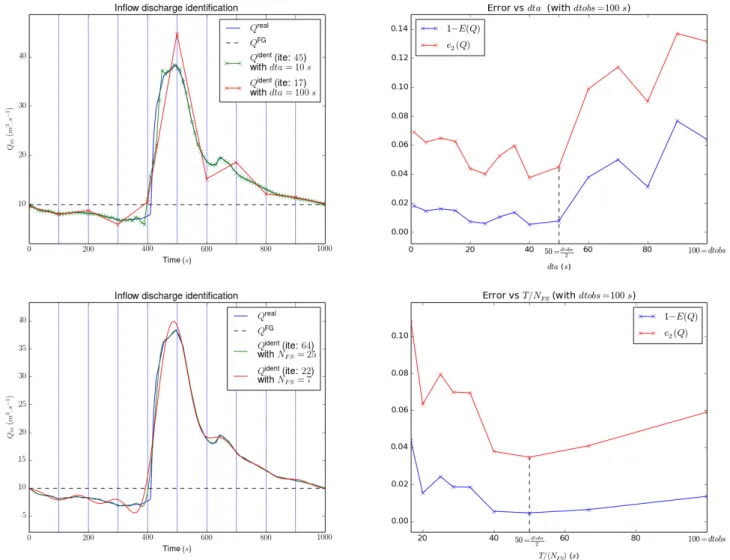
253
real case (Garonne river). The hydraulic propagation time Twave over the whole river domain equals ⇠ 160s for a 254
wave velocity (u + c) and the total simulation time is 1000s (cf.Table 1. Recall that Twave is of great interst when 255
using observations of water surface features within a river domain for identifying an inflow discharge (in x = 0). The
256
steady-state backwater curve, velocities and local Froude number values (Fr = pu gA
W
, with u =Q/Athe mean cross 257
sectional velocity) are presented on Fig. 2.2 for Qin= 10 m3.s 1 . The downstream boundary condition is a power 258
law rating curve defined by: hout(Q) = 0.45 Q0.6out (m). 259
260
Figure 2.2. Academic test case. (Left) Steady state flow for Qin= 10m3.s 1(quite a low value with
respect to the considered hydrograph in the forthcoming experiments): (Left, top) Water elevation H (Right, top) Discharge Q. (Left, Bottom) Froude F and (Right, Bottom) Velocity U vs river curvilinear abscissa. (Right) Cross-section example (for x = 500 m).
261
Academic test case Garonne river
mean µ [m/s] standard deviation [m/s] mean µ standard deviation
min(|u + c|) 6.3027 0.6063 5.4502 0.6805 mean(|u + c|) 6.3521 0.6224 6.0739 0.6561 max(|u + c|) 6.4028 0.6394 6.6827 0.8052 min(|u|) 1.3018 0.2916 0.7198 0.2507 mean(|u|) 1.376 0.2972 1.1023 0.1968 max(|u|) 1.4361 0.3069 1.391 0.2607
Hydraulic propagation time ⇠ 160 sec ⇠ 3.5 hours
Twave= mean(L|u+c|)
Table 1. Statistics on the wave velocity (u + c), velocity u and the hydraulic propagation time Twave
2.3.2. Garonne river test case. The 1D Garonne dataset contains a DEM of the river bathymetry between Toulouse
262
and Malause (South West of France, [51, 32, 18]) defined as follows:
263
• 173 cross sections measurements from the field, distant of 56 to 2200 meters with a median value of 438 m,
264
• a mesh containing 1158 cross sections; they result of linear interpolations of the original 173 cross sections,
265
• the cross sections are merged into lidar data of banks and floodplain elevations (5 m horizontal accuracy).
266
The mean slope of this 74 km portion of the Garonne River is 0.0866 % (86.6 cm/km ). The reference bathymetry is
267
the effective one respecting the trapezium superimposition structure as described in the academic case and preserving
268
the wetted areas, see figures 2.1 and 2.3. The considered bathymetry can be the reference one or the so-called
“low-269
Froude bathymetry” estimated from one (1) in-situ measurement and the method proposed in [18]. On the present
270
case it is those at the location x = 40 km (the reference point indicated in Fig. 2.1).
271
The effective SWOT like bathymetry (superimposition of trapeziums respecting the true wetted section values)
272
is compared to the Low Froude bathymetry (same trapeziums but not the same zb ) in Fig 2.3. The difference 273 1 N PN n=1|Zbtrue ZbLF| equals 38 cm. 274
The final mesh size, i.e. the spacing between interpolated cross sections extended on banks, is between 37.26 m and
275
70.0 mat maximum (the average spacing being 63.96m). The friction coefficient may be variable, depending on the
276
water depth. Its value is detailed in the identification experiment section.
277
The considered hydrograph is those measured at Toulouse during a 80 days period in 2010, see e.g. Fig. 5.2. In
278
terms of wave propagation, basic statistics are indicated in Table 1 and the hydraulic propagation time within the
279
whole river portion equals Twave⇠ 3.5 hours. 280
All the forthcoming numerical inversions can be performed from either the effective true value of bed level or from
281
the low-Froude one. Indeed the obtained results in terms of infered discharge and roughness coefficient are similar. The
282
assimilation of partial in-situ data in addition of the altimetry measurements is addressed into details in a forthcoming
283
study. Then the error pourcentages on the estimated discharge values in next sections are those obtained from the
284
effective true value.
285 286
Figure 2.3. Garonne data (Top) Effective bed elevation (zb mean slope) : the effective true value
(gray) and the low-Froude estimated value (blue). (Bottom) First cross sectional layer width w0 on
151 vertical layers, see Fig.
Remark 2. Concerning the unsual definition of K, an uniform power-law, see Eq. (2.2), it is worth to notice that the
287
forthcoming inversions performed by a VDA approach could have been done with a locally defined power-law Kr(h) 288
with r the “reach” number. However since the main goal of the present study is to focus on the identifiability of the
289
inflow discharge, in particular in terms of frequency flow variations, an uniform power law K(h) has been considered.
290
Moreover as it has been already mentioned, such a power-law gives already more degree of freedom than a mean
291
uniform constant value ¯Kas it is almost always considered in the literature.
292
2.4. The (SWOT-like) altimetric data . The identifiability capability of the present inverse method depends on
293
the spatial and temporal density of the water surface measurements. Synthetic SWOT observations are generated
294
over the studied domain (Fig. 2.4 ) from the expected SWOT ground tracks representing three temporal revisits over
295
the domain during a 21 days cycle. Then each swath (50 km wide) defined by the SWOT ascending and descending
296
tracks are split into 1 km stripes. These stripes define the so-called reaches; these splitting lenghts may related with
297
the physical flow features, see e.g. [17]. Only 25 stripes contain the considered Garonne river portions. These 25
298
observed reaches can be classified in 3 groups observed at different times Ti, i = 1..3within a 21 days satellite period 299
(see Eqn (2.10) and Fig. 2.4 ).
300
1D forward model outputs are averaged in space at each observation time ( ¯Hr(t)and ¯wr(t)) in order to reproduce 301
SWOT like observations at the reach scale; next a random noise is added in order to be representative of SWOT
302
observation errors averaged this reach scale.
303 304
Figure 2.4. Location of SWOT reaches on the Garonne river.
(Left) Aerial view from OpenStreetMap of Garonne River (black line) and SWOT reaches location with ascending (green) and descending (blue when the river is seen and red otherwise) tracks. (Right) Longitudinal river profile with the three groups respectively observed at T1= 12.58days, T2= 14.11
days and T3= 1.51days 305
2.5. Cost function. The cost function J to be minimized is defined from the available measurements as follows:
306
J(k) = jobs(k) + jreg(k) (2.7)
307
where jreg(k)is a regularization term defined later, and jobs(k)is defined by:
jobs(k) = 1 2 Z T 0 || ¯ Hk(t) Hobs(t)||2Wdt (2.8) 308
where ¯Hk(t)and Hobs(t)are defined by: 309 • ¯Hk(t) = ¯Hk 0(t), ¯H1k(t), ¯H2k(t), ..., ¯HNkr 2(t), ¯H k Nr 1(t) T 310
• Hobs(t) = H0obs(t), H1obs(t), H2obs(t), ..., HNobsr 2(t), H
obs Nr 1(t)
T 311
W is a symmetrical positive semi-define matrix Nr⇥ Nr, Nrthe number of observed reaches, and it defines an error 312
covariance matrix. Its extra diagonal terms wi,j, i 6= j, represent the correlation of error observations between reach 313
iand reach j; its diagonal terms wi,i are the a-priori confidence on the observation of reach i. In a real measurement 314
context, reaches close to the satellite nadir would be observed with lower errors. Hence, the diagonal coefficient values
315
should depend on the distance between the reach r and the nadir. Extra-diagonal terms are difficult to estimate and
316
considered to be null here. In all the following, the matrix W is the identity matrix of RN r (same confidence on all 317
observations).
318
The regularization term jreg(k)is defined by: 319
320
jreg(k) = jQreg(k) + jKreg(k)
321
where jQreg(k)(respectively j reg
K (k)) is the regularization term on the discharge (respectively the Strickler coefficient). 322
323
The balance coefficient between jreg(k) and jobs(k) can be classically set following the empirical Morozov’s 324
discrepancy principle and/or the classical L-curve strategy [38]. It will be observed in the numerical experiments that
325
no prior regularization needs to be considered on the friction term parameterized with a power law with constant
326
coefficients in space. Moreover, in the SWOT context, given the low frequency and high sparsity of the observations,
327
it is difficult (and numerically unnecessary) to define such a regularization term on Qin(t). This regularization may 328
be done by defining Qin(t) in the Fourier basis with frequencies a priori defined from the observation frequency, see 329
the discussion in the next section.
330 331
Let Nt,r denote the number of SWOT observation of the reach r. Then the discrete form of the cost function J 332
reads:
334 (2.9) J(k) = 1 2 X r=1,Nr X j=1,Nt,r ¯ Hr,jk H¯r,jobs 2 335 with ¯Hk r,j= ⌦1r P i=1,NrH k
i,jdx. With ⌦r the curvilinear length of reach r. 336
Let us remark that in an altimetry context, the ith observation time of reach group g, tg
i satisfies: 337
338
(2.10) tgi = i T + Tg
339
where T is the satellite period and Tg is the time lap of the first observation of the reach group g. Thus if a 340
river is observed by 3 satellite passes during 1 repeat period (like it is the case for the Garonne river, see Fig. 2.4),
341
then there are 3 different Tg (i.e. g = 1, 2 or 3). 342
All the equations and algorithms previously described have been implemented into the computational code DassFlow
343
[36]. It contains the 1D shallow water model dedicated to the altimetric data (effective cross section geometries) with
344
all required boundary conditions, a Strickler coefficient K(h) depending on the water depth plus a complete VDA
345
process. The adjoint equations are obtained by automatic differentiation [26] and the minimizer is a BFGS algorithm.
346
Note that few numerical schemes are possible: the classical implicit Preissmann’s scheme, the classical explicit HLL
347
finite volume scheme and also an original semi-implicit multi-regime scheme.
348
3. Discharge identification on the academic test case
349
This section aims at analyzing the inference capability of the 1D river Saint-Venant model from the water surface
350
observables described previously. As a first step, the unknown parameter is the inflow discharge Qin(t)only on the 351
academic channel described previously (Section 2.3.1). From the available observation distribution, (x, t)-identifiability
352
maps are calculated. They provide an overview of the inference capability of the forthcoming VDA process. These
353
maps are analyses in three contexts depending on three scenario of observation sparsity (see Fig. 3.1):
354
OD1: (Observation Distribution #1), the whole domain is observed (10 reaches),
355
OD2: the observations are available at upstream and downstream only (2x3 reaches), Fig. 3.1 (middle).
356
OD3: the observations are available in the middle only (4 reaches), Fig. 3.1(right).
357
Then the inference of Qin(t) is performed either classically by identifying its values on a fixed identification grid 358
(IDbasic case, with dta the constant assimilation time step), or by computing Qin(t)as a Fourier series (IDFourier 359
case). IDFourier case leads to a “global” computation of Qin(t)(on the contrary to the IDbasic). In both cases, an 360
analysis of the influence of the identification time grid is done.
361 362
Figure 3.1. Location of the observation reaches. (Left) Case OD1: the whole domain is observed (10 reaches). (Middle) Case OD2: observations are located at upstream and downstream (6 reaches). (Right) Case OD3: observations are located in the middle (4 reaches).
3.1. The identifiability map. This subsection introduces the identifiability maps. This map represents the
com-363
plete information in the (x, t) plane: the observations (the observed “space-time windows”), the hydrodynamic waves
364
propagation (1D Saint-Venant model) and the misfit to the “local equilibrium” (more precisely the local misfit with
365
the steady state uniform flow represented by the Manning-Strikler law). This preliminary analysis makes possible to
366
roughly estimate the time-windows which can be quantified by VDA since the inflow discharge values arise from these
367
observed “space-time windows”. This original reading of the hydraulic inverse problem is qualitative only but fully
368
instructive. Indeed this will make possible in the next section to roughly estimate whether the sought information has
369
been observed or not, in particular in terms of frequency (orders of magnitude).
The observations are generated from the hydrograph Qreal
in (t)shown in Fig. 3.3 Top-Left. Recall that the so-called 371
hydraulic propagation time Twave ⇠ 160 s (estimation based on the mean wave velocity (u + c)). From the hydraulic 372
propagation time and the observation time step dtobs (time between satellite overpasses), the identifiability index is 373 defined as follows: 374 375 (3.1) Iident= T wave dtobs 376
In the present case, dtobs= 100 s, hence lower than the hydraulic propagation time; the identifiability index Iident 377
⇠ 1.6. This means that at least the low frequency variations are observed.
378
An instructive analysis of the inverse problem consists to plot the so-called identifiability map in the plane (x, t).
379
Since the inflow discharge (that is Q(t) defined at x = 0) is the central sought “parameter”, the important wave
380
velocity is the positive one i.e. (u + c) in considering the Saint-Venant system waves. Indeed recall that without the
381
source terms (i.e. gravity waves model), the 1D Saint-Venant model wave velocities are (u c) and (u + c). Moreoiver
382
if considering the diffusive wave model, that is including the RHS of the Saint-Venant system, the wave velocity equals
383 5
3uin the case of a wide channel (see e.g. [12, 39, 52]and 1. 384
For each reach r (Nr = 10 in the OD1 case) and for each observation time tri (11 in the OD1 case), the velocity 385
waves of the 1D Saint-Venant model (and the diffusive wave model) are plotted, see Fig. 3.2. To do so, ¯ur i and ¯cri 386
corresponding to the reach r at time i are approximated; ¯u denotes the mean velocity value and ¯c = (g¯h)1/2(assuming 387
a rectangular cross section) with ¯h the mean water depth. Let us point out that in the present twin experiments, ¯u
388
is known. In a realistic context, ¯u can be estimated from a low complexity 0.5D model (Manning-Strikler’s equation
389
applied at each reach). Such estimations are sufficiently accurate to make the present analysis.
390
The (r, i) observation time interval is defined as follows: Tw
r,i= [tri Lr/(¯u + ¯c)ri, tri] with Lrthe reach length and 391
tr
i the observation time. Each observation space time window Tr,iw is plotted (in color) in Fig. 3.2. Each rectangle 392
diagonal corresponds to the local (¯u + ¯c) line; indeed the height of the rectangle Tw
r,i corresponds to (¯uri + ¯cri)⇥ Lr. It 393
can be noticed that the space-time variation of (¯u + ¯c) is not significant, see the rectangle height variations and Table
394
1.
395
In the present case, the whole domain is observed at t = 0 hence the wave velocity (¯u + ¯c) at t = 0 can be estimated
396
accurately.
397
The identifiability map in (x, t) is plotted for the three cases depending on the observation sparsity: cases OD1,
398
OD2 and OD3, see Fig. 3.2.
399
The rectangle colors represent the misfit to the steady uniform flow (in norm 1). It is the right-hand side (the
400
source term) in norm 1 of the momentum equation, see (2.1):
401
(3.2) "Steady uniform flow misfit" = Norm1[ g
Z h 0 (h z)@ ˜w @xdz gS( @zb @x + Sf) ]
If this source term vanishes (blue colors in Fig. 3.2), it means that locally in space and time the flow variables satisfy
402
the steady state uniform flow equation (here the Manning-Strikler equation). On the contrary, if the misfit term
403
becomes important (e.g. orange - red colors) then the hyperbolic feature of the model is important.
404
In terms of energy, this non-conservative source term contains the dissipative friction term Sf; while the left-hand 405
side of the 1D Saint-Venant model is conservative, see (2.1). Therefore Fig. 3.2 provide a rough estimation of the
406
propagation features of the flow model including advection diffusion phenomena.
407
Typically, the peak time at inflow is represented by the rectangle (r, i) = (1, 6). The corresponding wave velocity
408
(¯u + ¯c) is faster than those arising from the middle of the domain for example, see rectangle (6, 6).
409
To illustrate differently the advective-diffusion phenomena corresponding to Fig. 3.2, the discharge throughout the
410
domain is plotted at the three observations times 400s, 500s (peak time at inflow) and 600s in Fig. 3.2 Top Right.
411
All these information represented in the (x, t) plane constitute the so-called identifiability map. Its analysis provides
412
a comprehensive overview of the inversion capability, in particular with respect to the inflow discharge Qin(t). 413
If a characteristic (¯u + ¯c) line crosses one or more observed reaches (the colored rectangles on Fig. 3.2), the
identifi-414
ability of discharge is ensured at the time corresponding approximately to the intersection between the characteristic
415
and the vertical axis. In other words, for a reach observed at time tr
i and abscissa rLr, the inflow discharge should 416
be identifiable at time ⇠ (tr
i rLr/(¯u + ¯c)). Typically, in the present case, the identifiability maps show that any 417
change on Qinis observed at least few times, and this is true for the three scenarios OD1, OD2 and OD3. In other 418
words, there is no blind time-space window; the same hydraulic information may be observed even few times. Then
419
the forthcoming identification computations based on VDA will be robust and accurate for the complete simulation
420
time range [0, T ].
421
This a-priori analysis is confirmed by the VDA experiments presented in next paragraphs.
422
Remark 3. The present source term estimation provides an a-posteriori model error if employing the usual
Manning-423
Strikler’s law to model the flow.
424 425
Remark 4. It can be noticed that since the wave velocity 3u¯ is slower than (¯u + ¯c), see Fig. 3.2. Following the
426
same analysis, it shows that the inflow discharge identifiability in the diffusive wave model would be higher than in
427
the present 1D Saint-Venant model. However if considering a wave velocity value or another, the present analysis
428
remains qualitatively the same; while the quantitive conclusions would differ slightly. The present identifiability map
429
has been arbitrarily plotted using the Saint-Venant waves velocities (recall, values valid if not considering the RHS).
430
For a comparison between the diffusive wave model and the present Saint-Venant model, see e.g. [39] and references
431
therein.
432 433
Figure 3.2. The identifiability maps in (x, t) in the case: (Top, Left) OD1 (full observations); (Bottom, Left) OD2; (Bottom, Right) OD3.
The estimated wave velocities are plotted in red (continuous line) for the 1D St-Venant model (u + c), and in green for the diffusive wave model (5
3u). The red dotted line represents outgoing wave velocity¯
(u c) (on the Fig., from the reach r=6 at observation instant i=6). The “steady uniform flow misfit” defined by (3.2) is represented in each rectangle by the colors.
(Top, Right). Discharge Q(x, ·) vs x at three observations times: 400s, 500s (=the peak time at inflow), 600s.
434 435
3.2. Identification for various dta. In this section, assuming that both the river bathymetry and the friction law 436
are given, few identifications of inflow discharge are performed with :
437
• a fixed observation time step dtobs= 100sand various assimilation time steps dta, ranging from 1/10 to 1 dtobs 438
- IDBasic case in Section 2.1. The parameter vector is k = (Q1, ..., Qp)T with dta= (ti+1 ti) = 8i 2 [1..p 1]. 439
• Qin(t)represented in a reduced basis (Fourier series, see (2.3) - IDFourier case in Section 2.1. The parameter 440
vector reads: k = (a0, a1, b1..., aNF S, bNF S)
T and the identification with VDA of N
F S = 7 and NF S = 25 441
Fourrier coefficients is tested.
442
The inflow discharge and the gradient value are plotted in Fig. 3.3 Top, for IDBasic case with dta = dtobs/10 and 443
dta= dtobs. In the case dta= dtobs/10the result is excellent, and if dta= dtobsthe accuracy remains good (excepted 444
at peak time, t ⇡ 500s) - convergence reached in 45 and 17 iterations respectively.The errors on the identified inflow
445
discharge are plotted in Fig. 3.3. Both the 2-norm error and (1 E), with E the Nash–Sutcliffe criteria, are the
lowest for dta between 20 s and 50s = dtobs/2(with (1 E) ⇠ 0.0077). Roughly, the error is improved if dta < dtobs 447
but dta not too small. Indeed, for dta << dtobs, typically dta= dtobs/10, over and under estimations of the discharge 448
appear. Indeed, if dta is small, any change of Qinbetween two identification times, is not observed, Fig. 3.3 Left-top. 449
The value obtained for dta = dtobs/2is almost the optimal value. As a practical guide, a simple rule would be to set 450
dta= dt2obs i.e. consider one intermediate point only between two observations. 451
For IDFourier case roughly the same accuracy and behaviors as in the previous case are obtained, see Fig. 3.3
452
Bottom. Indeed the minimal error, (1 E) ⇠ 0.005, is obtained with T/NF S ⇠ dtobs/2. Again, as a practical guide, 453
a simple rule would be to set NF S such that T N F S =
dtobs
2 i.e. considering one intermediate point (and only one) 454
between two observations, Fig. 3.3.
455
The advantages of identifying Qin(t)as a Fourier series are the following: the control vector is smaller, the frequency 456
imposed a-priori can be quite easily estimated, and the identified inflow discharge remains smooth (this circumvents
457
the potential oscillations obtained in the case IDbasic with dta<< dtobs for example). 458
459
Figure 3.3. (Top) Discharge identification: IDbasic approach with dtobs = 100 s. (Left, top)
Dis-charge identification with dta = dtobs = 100 sand dta = dtobs/10 = 10 s. (Right, top) Normalized
gradient rQJ with dta = dtobs and dta = dtobs/10 = 10 s. (Middle) Errors vs dta; dta = dtobs/2
is almost the optimal value. (Bottom) Discharge identification: IDFourier case (Fourier series recon-struction) with dtobs= 100 s: (Bottom Left) Discharge identification with NF S = 7and NF S= 25.
(Bottom Right) Errors vs T/NF S
3.3. Identification robustness vs observation sparsity. A VDA process is global in time. The previous numerical
460
experiments demonstrate that refining too much the identification time grid dta compared to dtobs (typically dta = 461
dtobs/10) deteriorates the identification accuracy. In other words, given an observation time grid, the identification 462
of the time dependent inflow discharge cannot be obtained at much finer time scale. All these previous experiments
463
have been performed with observations available on the whole domain (case OD1, see Section 3). In a real case (e.g.
464
SWOT data of Garonne river test, see Section 2.4) the observations are not available for the whole domain, nor all
at the same time. Thus in the present experiments, the robustness and accuracy of the discharge identification is
466
investigated if considering real-like SWOT data hence much sparse observations.
467
The inflow identification are performed with a pseudo-optimal assimilation time step dta= 25 s (still with dtobs= 468
100 s) for the three cases OD1, OD2, OD3, see Fig. 3.1.
469
As discussed in Section 3.1, the identifiability maps (see Fig. 3.2) indicate that in the three cases the identification
470
should be accurate. Indeed, the numerical results obtained by VDA confirm this a-priori analysis since the error is
471
extremely low, typically E > 0.99, see Tab. 2. The identified inflows are not plotted since the results are similar to
472
the previous case.
473 474 475
OD 1 OD 2 OD 3
Nash-Sutcliffe coefficient (E) 0.993 0.994 0.991
Table 2. Academic test case, Nash-Sutcliffe coefficient (E) for dta= 25 sin function of the
observa-tions availability: cases OD1, OD2, OD3.
4. Discharge and roughness identification in the academic test case
476
In the previous section, Qin(t)only was infered. In the present section both the time-dependent inflow discharge 477
and the Strickler coefficient K (time-independent) are infered by the VDA process. Let us recall that K is defined
478
by: K = ↵h . Then the control vector reads: k = (Qin,1, Qin,2, ..., Qin,p, ↵, )T in the IDbasic case and k = 479
(a0, a1, b1..., aNF S, bNF S, ↵, )
T in the IDFourier case. In the present experiments the bathymetry is given. The 480
synthetic observations are generated from the same hydrograph (inflow discharge) as previously and an uniform
481
coefficient K = 25 i.e. ↵ = 25 and = 0 in Eqn (2.2). First guesses are respectively chosen equal to Qin(t) = 482
100 m3.s 1 for all t, and to (↵, ) = (23.5, 0.1) (hence considering K depending on h). The observations are available
483
in the whole domain: OD1 scenario.
484
4.1. Identifications in the IDbasic and IDFourier cases. The identified inflow discharge with a basic linear
485
reconstruction (IDbasic case) is as accurate as in the previous case i.e. while identifying Qin only. The identified 486
discharge are plotted in Fig. 4.1 Left top in the case dta= 10 sand dta = 100 s. 487
For dta = 10 s, the identification of the roughness parameters ↵ and is accurate, see Fig. 4.1 Bottom; the 488
minimization algorithm has converged in 64 iterations. For dta = 100 = dtobs, the minimization algorithm has more 489
difficulties to converge, see Fig. 4.1 Top right. In the IDFourier case, the results are similar.
490
In both cases (IDbasic and IDFourier), the identified quantities are accurate if the identification time step dta is 491
small enough compared to dtobs, or if the Fourier mode number NF S is large enough. In such cases, the identification 492
of Qin(t)is as accurate and robust as in the previous case (when Qin(t)only was identified). 493
But if dta= dtobsor equivalently if NF Sis small, then the minimization algorithm has more difficulties to converge, 494
hence the VDA process provides less accurate quantities.
495
The errors on the roughness coefficients are plotted in Fig. 4.3. Since the error made on the identified discharge
496
are very similar than in the previous case they are not plotted. The value of dta (resp. NF S) such that dta= dtobs/2 497
(resp. T/NF S = dtobs/2) are almost the optimal values. Thus the basic practical rule consisting to set the assimilation 498
frequency equal to the double of the observation frequency is relevant.
499 500 501 502
4.2. Sensitivity of identifications to first guesses and observation errors. The sensitivity of the identified
503
quantities (Qin(t)and (↵, )) with respect to the first guess values Qin,F G and (↵, )F G is investigated: OD1 case 504
(complete spatial observations), IDFourier case with NF S = 20. For each sensitivity map representing identification 505
errors in the space of first guess values of ↵ and Qin( Fig. 4.4) the parameter is fixed ( = 0). They show that the 506
identification of inflow discharge Qin(t)and the roughness coefficients are accurate for a large value range of Qin,F G. 507
However the accuracy is important for low values of Qin,F G. Thus it is preferable to over estimate the first guess 508
(hence starting from high water levels) than under estimate it. The results are very similar if the fixed parameter is
509
the discharge Qinor the roughness law parameter ↵, then the corresponding figures are not presented. 510
Finally the impact of observation errors on the three identified quantities are presented in Fig. 4.5. A Gaussian noise
511
N (0, ) is added to the water elevation data Hobs. In the case = 0.1 m (this corresponds to the expected error of the 512
forthcoming SWOT instrument, cf. [46]), the error on the roughness law parameters (↵, ) equals approximatively 5%
513
and the Nash–Sutcliffe criteria E ⇡ 0.5. In a bad observational context with = 0.5 m, the error on the roughness law
514
parameters (↵, ) equals approximatively 10 25% and the Nash–Sutcliffe criteria E(Q) becomes negative. Therefore,
Figure 4.1. Discharge and roughness identification in the academic test case (IDbasic case). (Left, top) Discharge identification with dta = dtobs = 100 s and dta = dtobs/10 = 10 s. (Right, top)
Function cost J,||rQJ||,||r↵J|| and ||r J|| vs minimization iterations. (Left, bottom) Roughness law
coefficient ↵ vs minimization iterations. (Right, bottom) Roughness law coefficient vs minimization iterations.
the identification of the composite control parameter (Qin(t); K(h))turns out to be quite sensitive to the observation 516
errors but its inference remains accurate in the case of a SWOT-like accuracy ( = 0.1 m).
517
518
Figure 4.2. Discharge and roughness identification in the academic test case (IDFourier case). (Left) Discharge identification with NF S = 7 and NF S = 25. (Right) Function cost J,||ra0J||,||ranJ||,
||rbnJ||,||r↵J|| and ||r J|| vs minimization iterations.
Figure 4.3. Roughness identification in the academic test case: errors e2 on the coefficients (↵, ).
(Left) IDbasic case: errors vs dta. (Right) IDFourier case: errors vs T/NF S.
Figure 4.5. Error on the identified quantities with k = (a0, a1, b1..., aNF S, bNF S, ↵, )
T
vs the observation error (standard deviation of the Gaussian noise). The vertical dashed line represents the expected error of the SWOT mission, both in norm 2 and Nash-Sutcliffe criteria.
Figure 4.4. Sensitivity to the first guess: errors on the identified quantities vs ↵F G and Qin,F G (
is fixed). (Left, top) Error e2(↵). (Right, top) Error e2( ). (bottom) Error on Qin: Nash–Sutcliffe
criteria E.
5. Garonne river test case
520
The accuracy and the robustness of the VDA process, see sections 2.2 and 2.5, is investigated in a realistic data
521
context. The test case is the Garonne river (portion downstream of Toulouse) described in Section 2.3.2. The
522
considered hydrograph is presented on Fig. 5.2. The SWOT-like observations are generated by the model following
523
the method presented in Section 2.4. For the VDA computations the first guess Qin,F Gis chosen constant and equal 524
to 268 m3/s(the mean value of the true hydrograph), see the horizontal dotted lines in the inflow discharge graphs, 525
Fig. 5.2.
526
As a first step and following Section 3.1, the identifiability maps are computed. Scenario 1 (Section 5.2) consists to
527
consider a SWOT temporal sampling as defined in Section 2.4. The repeat period is 21 days and the simulation time
528
is T = 80 days. Scenario 2 is based on a densified SWOT temporal sampling by a factor 100: the repeat period is 0.21
529
day and the simulation time T = 0.8 day. This theoretical scenario would correspond to a combination of observations
530
provided by different satellites. Also during the SWOT CalVal period (the first weeks after the launch), the satellite
531
will be on a lower orbit and will offer a ⇠ 1 day repeat period on some rivers.
532
It has been shown in the previous section (academic test case) that the error made on the identified inflow discharge
533
Qin(t)is similar if identifying Qin(t) only or the composite control vector (Qin(t), K(h)). Moreover still in terms of 534
error on the identified inflow discharge Qin(t)only, the accuracy obtained from the true effective bathymetry or from 535
the low Froude effective bathymetry are very similar. Obviously the corresponding identified value of K(h) differ
536
between the two cases. This illustrates again the equifinality issue related to the bed properties, that is the pair
537
(bathymetry, friction).
538
Observe that the VDA process could be performed for the complete unknown parameter (Qin(t), K(h))and Zb(x) 539
(this has been done and its fine analysis is out of the scope of the present article). However, it may be not the best
540
strategy to calibrate a river dynamic flow model since the equifinality issue on the bed properties (K, Zb). That 541
is the reason why in the present study we do focus on the inversion with respect to Qin(t) (or equivalently with 542
respect to (Qin(t), K(h))), and we investigate into details the reliability and accuracy of the obtained results. The 543
eqbathymetryuifinality issue is complex; it is the main purpose of an on-going study and likely next article.
544
5.1. Identifiability maps. The identifiability maps are computed from the observations following the method
de-545
scribed in Section 3.1 for both scenarios, see Fig. 5.1. On the contrary to the academic test case, no observation is
546
available at t = 0 hence the wave velocity (¯u + ¯c) propagating from t = 0 cannot be estimated. Fig. 5.1 Left shows
that in the SWOT sampling case, the identifiability of Qin(t)is approximatively limited to the observation “day time”, 548
hence preventing to infer in-between inflow variations (since no constraining information). The lack of constraining
549
observation is accentuated here since a single quite short river portion is considered with its hydraulic propagation
550
time Twave ⇠ 3.4 h only, see Tab. 1, hence an extremely low identifiability index Iident⇠ 6.7 10 3. 551
The next scenario (Scenario 2) is a 100 times greater revisit frequency: dtobs = 0.21 day. Keeping the same 552
hydrograph but rescaled in time, the hydraulic propagation time Twave is the same (⇠ 3.4 h) but the observation 553
frequency equals 0.21 day, hence the identifiability index is 100 times greater: Iident ⇠ 0.67. This rough analysis 554
informs that almost the complete wave set traveling within the river portion should be captured by the sensor.
555
In the identifiability maps Fig. Fig. 5.1 the inflow discharge identifiability is represented by the vertical dashed lines
556
at x = 0: in red the characteristics feet provided from the “far” green observed reaches (hence an identifiability likely
557
less accurate); in black the characteristics feet provided by the “close” blue observed reaches (hence an identifiability
558
likely very accurate).
559
Recall that this identifiability analysis is based on the wave velocities estimations only, while the dissipation due to
560
the friction source term is not taken into account. However these maps indicate that in Scenario 2 a large proportion
561
of inflow values should be accurately identifiable (see the vertical points at x = 0).
562
The forthcoming VDA experiments confirm this a-priori analysis; the dashed vertical lines (red and black) on Fig.
563
5.1are taken back on the identified discharge graphs on Fig. 5.3.
564 565
Figure 5.1. Identifiability maps in the Garonne river case: (Left) Scenario 1 (SWOT like, 21 days repeat) (Right) Scenario 2 (100 times more frequent, 0.21 day repeat). The circles centered at t ⇡ 0.45 days correspond to the inflow peak. .
In Scenario 1, the identifiability index Iidentis so tiny that all the characteristics are almost horizontal
and the identifiable times at x = 0 corresponds roughly at the “observation day”.
In Scenario 2, the velocity waves (¯u + ¯c) (dotted lines) are estimated at each reach from the available observations (see sections 3.1 and 5.1). The rectangle heights are proportional to the local value (¯u+¯c). The dashed vertical lines at upstream represent the characteristic feet i.e. the sets of points which can be identified in the model without the dissipative source term: in red the information coming from the “far” green observed reaches (hence an identifiability likely less accurate); in black the information coming from the close blue observed reaches (hence an identifiability likely very accurate). These dashed vertical lines (red and black) are taken back from the identified discharge graphs Fig. 5.3.
5.2. Scenario 1: real SWOT temporal sampling. The Strickler coefficient K and the bed level zbare given. The 566
latter is either the effective true bathymetry or the bathymetry estimated by the low-Froude equation presented in
567
[18] and one (1) in-situ measurement. The numerical results presented below are those obtained with the effective
568
bathymetry estimated from the low-Froude equation and the exact lowest wetted area at x = 40 km (the so-called
569
reference point in Fig. 2.1). Next the inflow discharge is identified by VDA from the real SWOT space time sampling.
570
Following the preliminary study based on the identifiability map, Qin(t) is decomposed as a Fourier series(IDFourier 571
case) with NF S= 5(Fig. 5.2 Left) and NF S = 10(Fig. 5.2 Right). Then as expected, the identification is accurate 572
in the vicinity of each observation (the vertical colored lines in Fig. 5.2) but inaccurate elsewhere. Indeed, norm 2
573
of the identified discharge at observation times is eT obs
2 ⇠ 16.5% and e2 ⇠ 42% if considering the whole hydrograph 574
(more precisely 41.4% for NF S = 5 and 54.5% for NF S = 10).As expected increasing the identification frequency
575
(case NF S = 10) does not improve the coarser approximation (NF S = 5) since the latter already corresponds to an 576
adequate frequency compared to the observation mean frequency, see Fig. 5.2.
577
As already discussed, the identifiability index is extremely small (Iident ⇠ 6.7 10 3). This very small index value 578
is due to the important spatiotemporal sparsity of the data and a short river portion (74 km). However the VDA
process makes possible to infer quite accurately the inflow discharge roughly at observation day times, but the too
580
small identifiability index prevents to constraint the inflow discharge between the observation times.
581
All these results corroborate the a-priori analysis made from the identifiability map.
582
Let us point out that in a complete river network, each observation (at a given location and a given time) is spread
583
into the whole network model (at the various wave velocities) if the hydraulic propagation time is larger than the
584
observation frequency (i.e. with a identifiability greater than 1). Then each satellite overpass can constraint the
585
lowest frequency of the inflow hydrograph in the network.
586 587
Figure 5.2. Garonne river, Scenario 1. Discharge identification with Fourier series with: (Left) NF S= 5, eT obs2 (Qestimatein ) = 17.1%. (Right) NF S= 10, eT obs2 (Qestimatein ) = 16.2% .
Vertical lines corresponds to the time observations (blue for Group 1, red for Group 2 and green for Group 3). The horizontal dotted line corresponds to the first guess Qin= 268 m3/s.
588
5.3. Scenario 2: densified SWOT temporal sampling by a factor 100. In the present case, the data sampling
589
and the hydrograph are re-scaled / densified in time by a factor 100. The numerical inversions are strictly the same
590
as the previous ones but the time scale and the values of NF S.
591
The re-scaled hydrograph remains consistent with the domain length since the peak duration is higher than the
592
response time of the whole river portion; recall Twave⇠ 3.4 hours. The identifiability index Iident⇠ 0.67. 593
As indicated on the identifiability map Fig. 5.1, a majority of the inflow information is observed since it has time
594
enough to travel throughout the domain. This suggests that the inflow values are in majority accurately identifiable
595
but are not during some (a-priori short) time intervals. These more or less accurate time intervals are indicated as
596
the black and red dots in Fig. 5.1 and Fig. 5.3.
597
The VDA results are presented on Fig. 5.3, read e.g. the case NF S = 10, Left-Bottom. The values at the times
598
corresponding to the black identifiability intervals are accurate (as expected). The norm 2 error at observation times
599
equals ⇠ 4.5%. On the contrary, the peak is partially captured only since it occurs during a red identifiability interval
600
(see the red dots on Fig. 5.1 and Fig. 5.3). However, the identification is globally correct considering the quite low
601
identifiability index Iidentvalue of the scenario. Indeed the index is strictly lower than 1, hence suggesting some “blind” 602
time intervals in terms of identifiability.
603
As indicated in Fig. 5.3), the VDA process is performed for four values of NF S= NF S = 5, 10, 15 and 40. In
604
the numerical method, the value of NF S has to be a-priori set. This can be easily done from the identifiability map
605
analysis and the dtobs value. Indeed it has already been suggested that setting NF S such that: T/NF S ⇠ dtobs/2 606
(which corresponds here to NF S ⇠ 8 ) should be quite optimal.
607
In view to fully analysis the sensitivity with respect to the NFS value, the results obtained from for the four values
608
above are compared. Moreover, to better understand the origin of the identification errors, the approximation of the
609
exact inflow discharge Qtarget
in (t)by the same Fourier series is plotted in each case, see the four curves “Exact FS with 610
NFS=...” in Fig. 5.3. This makes possible to analyze the error origin from the Fourier series approximation and from
611
the VDA process (with respect to the present index value ).
612
The best results is obtained with NFS equals to 10 (the case 15 is good too), providing an error at observation
613
times ⇠ 4.2%, and ⇠ 20% if considering the whole hydrograph, see Fig. 5.3. All errors are detailed in the title of Fig.
614
5.3.
615 616