Monitoring of fields using body and surface waves reconstructed from passive seismic ambient noise

HAL Id: hal-02931569

https://hal.univ-grenoble-alpes.fr/hal-02931569

Submitted on 10 Sep 2020

HAL is a multi-disciplinary open access

archive for the deposit and dissemination of

sci-L’archive ouverte pluridisciplinaire HAL, est

destinée au dépôt et à la diffusion de documents

Monitoring of fields using body and surface waves

reconstructed from passive seismic ambient noise

Florent Brenguier, Aurélien Mordret, Richard Lynch, Roméo Courbis, Xander

Campbell, Pierre Boué, Malgorzata Chmiel, Shujuan Mao, Tomoya Takano,

Thomas Lecocq, et al.

To cite this version:

Florent Brenguier, Aurélien Mordret, Richard Lynch, Roméo Courbis, Xander Campbell, et al..

Mon-itoring of fields using body and surface waves reconstructed from passive seismic ambient noise. SEG

International Exposition and 89th Annual Meeting, Sep 2019, San Antonio, France. pp.3036-3040,

�10.1190/segam2019-3216217.1�. �hal-02931569�

Technology; Tomoya Takano, Tohoku University; Thomas Lecocq, Royal Observatory of Belgium; Wim van der Veen, Nederlandse Aardolie Maatschappij; Sophie Postif, Shell International Exploration and Production; Dan Hollis, Sisprobe.

Summary

There are important economic, environmental and societal reasons for monitoring production from oil, gas and geothermal fields. Unfortunately, standard microseismic monitoring is often not useful due to low levels of microseismicity. We propose to use body and surface waves reconstructed from ambient seismic noise for such monitoring. In this work, we use seismic data recorded from a dense sensor array at the Groningen gas field in northern Holland and show how direct P-waves can be extracted from the ambient noise cross correlations and then used to monitor seismic velocity variations over time. This approach has advantages over the use of coda wave interferometry due to the ability to localise such changes in the subsurface. We show how both direct and refracted (head) P-waves as well as Rayleigh surface waves can be used for such field monitoring, with changes of ~1% being resolved. Both fundamental and first overtone Rayleigh waves are used to localise such changes, which correspond nicely to known geology to within 100 m.

Introduction

Monitoring of oil, gas and geothermal fields during production is important for economic and societal reasons. While microseismic monitoring is widely used for monitoring of the stimulations and early production [Shapiro, 2008], the typical drop in recordable microseismicity afterwards reduces the value of this technique [Shoenball et al, 2014]. In particular, the aseismic deformations that can indicate potentially unwanted leakage and in some cases corresponding contamination of aquifers are difficult to monitor [Rutqvist, 2012].

Noise-based passive seismic methods can potentially add much value for reserviour monitoring. These methods are based on the proportionality of the Green’s function with the cross-correlation noise seismograms recorded in a diffuse seismic wavefield [Lobkis and Weaver, 2001; Shapiro and Campillo, 2004; Roux et al, 2005; Campillo, 2006; Snieder, 2007].

Different studies have showed that body-wave extraction from noise correlations is possible at various scales (Roux et al. 2005, Draganov et al. 2009, Poli et al. 2012). Nakata et al. (2015) were able to implement the first passive 3-D P-wave velocity tomography from continuous ground motion recorded on a dense array of more than 2500 seismic sensors installed at Long Beach (California, USA). Recently Brenguier et al. (2016) and Nakata et al. (2016) showed the temporal stability of direct virtual body-waves between dense arrays on Piton de la Fournaise volcano thus opening the way for continuous, passive ballistic wave monitoring.

Method

The new approach is based on measuring temporal changes of apparent slowness of specific ballistic waves that have been reconstructed from noise correlations using dense arrays of seismic sensors (Boué et al., 2013, Mordret et al. 2014, Nakata et al., 2015, Nakata et al., 2016). The underlying requirement is for a high number of seismic sensors (> 100) and if satisfied the noise correlation receiver pairs allow for the reconstruction of a virtual shot-gather of sufficiently high quality to be able to isolate and measure the apparent velocity of ballistic waves such as direct P or S-waves, refracted waves or surface waves with clear mode separation.

In this study, we gather all possible noise cross-correlations from every sensor pair in a dense array into a single data set – propagation time vs virtual source offset – and thus assume a 1D horizontal velocity model. Then we measure the arrival time variations of identified body wave types at each offset, and use a linear regression to measure the velocity variation across the array for each time interval. In this way time lapse monitoring is achieved for each identified body wave, as illustrated in Figure 1.

Data

The Groningen gas field located in the northeast of the Netherlands is one of Europe’s largest natural gas fields. The reservoir is located at 3 km depth and is thought to be 40 by 50 km wide and 250 m thick. It is sealed by an overlying Zechstein salt layer up to 1 km thick. Above the

Ambient Noise Passive Seismic Monitoring

salt layer lies a 1 km thick Cretaceous Chalk formation! capped with a 800 m thick Tertiary and Quaternary sediment cover, up to the surface (van Thienen-Visser & Breunese 2015).

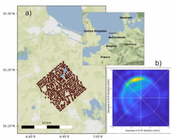
We are using continuous seismic data recorded by a network of 417 short period triaxial (3C) geophones deployed in the Groningen area (Figure 2) from 11 February (day 42) to 12 March (day 71) 2017. The network forms a grid array with aperture of the order of 8 km and typical inter-sensor distance of about 300 m.

Direct and Refracted P-waves

After the cross correlation of the vertical components of the seismograms and the binning procedure previously outlined, we obtain images shown in Figure 3 for different frequency bands. The dominant waves present, particularly at low frequency, are the surface waves but P-waves are also clearly present – especially at higher frequencies. The P-waves are present on the vertical components due to the velocity gradient near to surface which causes the P-waves to travel horizontally as a series of ‘smile’ curves with vertices from reflections off the free surface.

The high frequency (3-12 Hz) window reveals both ‘direct’ P-waves travelling at 1700 m/s (which is roughly the known P-wave velocity in the top 700m layer) and refracted P-waves travelling with a velocity of about 3000 m/s. We interpret this refracted wave as a head wave from the P-waves travelling beneath the interface, and thus this observed velocity is the P-wave velocity of that layer.

Having identified the inter-station distance window where the direct and the refracted P-waves are clearest, we build a reference image by stacking the virtual gathers from days 42-50. Then we use a sliding 10-day window to make similar images and compare against the reference to extract velocity changes for each inter-station distance. A linear fit to the velocity changes at each inter-station distance yields the velocity change at that time. This procedure is repeated for both direct and refracted P-wave: the images for the refracted wave is shown in Figure 4, and resulting velocity change over time for both P-waves is shown in Figure 5.

Figure 2: a) Geometry of the 417 short-period geophones used in this study. b) beamforming of the 30 days of continuous seismic data in the 1-4 s period range. The noise is coming from the North, mostly likely from the shore about 20 km away.

Figure 3: Noise cross-correlation averaged binned section from vertical sensor components for frequency ranges 1- 3 Hz (top) and 3-12 Hz (bottom). The blue and red dashed boxes in the bottom image correspond to the selected windows used for the analysis for the direct and refracted waves. The right panel illustrates the average P-wave velocity model of the area illustrating the velocities of the overburden (saturated sediments) around 1700 m/s and of the chalk layer at ~750 m depth around 3000 m/s. Figure 1: Procedure for ballistic-wave apparent seismic velocity

monitoring. a) propagation of a direct ballistic wave. The dashed lines show the reference wave and the plain lines show the wave affected by a velocity perturbation of -7 %. b) travel time shifts measurements and linear regression along distance. c) conversion from distance to travel time by dividing distance by V, the apparent velocity of the propagating wave.

Rayleigh Waves

As previously mentioned, the cross correlated waveforms exhibit strong surface (Rayleigh) waves on the vertical components. Actually, both the fundamental and first overtones are clearly visible (Figure 6) and thus used in this analysis, after a suitable F-K filter is used to separate them.

As before, a reference cross-correlation is used to compare against the daily cross-correlations, and then used to extract phase velocity variations for each day as functions of inter-sensor distance and frequency. As we use all inter-sensor-pairs, we are implicitly assuming a 1D velocity model. A linear fit is applied to the changes as a function of inter-sensor distance, in a window of between 3 and 7 wavelengths to allow the surface waves to fully develop and to avoid high distances where data is sparse and measurement less reliable. In this way we obtain surface wave changes for each frequency band for each day.

We then make a depth inversion for each day, using the frequency-dependent changes and both fundamental and first overtone data. It’s worth noting that the sensitivity kernels (Figure 7) for these frequency bands show different depth dependencies and so the first overtone data

Figure 4: a) Reference image from windowed refracted P-waves averaged for the time period (days 42 to 50). b) current image from windowed refracted waves averaged for days 48 to 57. c) travel time shift measurements as a function of inter-sensor distance from these two refracted waves.

Figure 5: Apparent seismic velocity temporal changes for both the direct a) and refracted b) waves. Note vertical axis scale change.

Figure 6: a) Full seismic section filtered between [0.6–1.2] Hz. The inset shows the phase velocity dispersion curves of the fundamental mode (blue) and the first overtone (red). b) FK diagram of the seismic section. The FK filter windows to extract the fundamental mode and the first overtone are shown in red and yellow, respectively. c) The FK-filtered fundamental mode band-pass filtered between [0.6–1.1]Hz. d) The FK-filtered first overtone band-pass filtered between [0.4–1.0]Hz.

Ambient Noise Passive Seismic Monitoring

significantly improve the inversion. After the inversions, we have a 1D S-wave velocity model for each day, which we present in Figure 8.

Observations

The direct and refracted body waves (Figure 5) show that while the near-surface P-wave velocity is not significantly changing in the 30 day recording period, the velocity of the Chalk layer beneath 800 m depth does increase by +1.5% around day 54-56. This level of change is more than double the measurement error. After day 55, the Rayleigh wave analysis indicates a significant decrease of around 1.5% in the zone below 800 m depth. It should be noted that these two methods are quite different, using the same seismic noise data but different waves and processing. With that in mind, the common timing and location of the indicated subsurface changes is remarkable.

The recorded noise characteristics (directionality and spectrum) are stable in the 30-day period, ruling this out as a cause of the indicated velocity change. INSAR and GPS data do not suggest any causes, and neither does gas production data and modelling - these induced pressure variations are of the order of less than 0.1 MPa locally and are thus too small to potentially induce a 1.5 % velocity increase 2.3 km above in the carbonate layer. We also rule out the effects of local induced earthquakes due to the low level of seismicity during the studied time period. The only significant weather event was heavy rain (40 mm) over days 54-56, and so this is suggestive as the origin of the surface changes (P-wave +1.5%, S-wave -1.5%) at 800 m depth in the days following it.

Conclusions

We have demonstrated how ambient seismic noise – vibrations from trains, cars, ocean, etc. – recorded by a dense array of surface sensors can be used to reconstruct both body waves and surface waves, which can then be used to monitor subsurface changes in a gas (or oil or geothermal) field during production. These results suggest a new, cost-effective way of monitoring such fields. Acknowledgements

This project received funding from the Shell Game Changer project HiProbe as well as support from the French ANR grant T-ERC 2018, (FaultProbe), the European Research Council under grants FAULTSCAN and no. 742335, F-IMAGE and the European Union’s Horizon 2020 research and innovation program under grant agreement No 776622 (PACIFIC). AM acknowledges support from the National Science Foundation grants PLR-1643761. The data were provided by NAM (Nederlandse Aardolie Maatschappij). We acknowledge M. Campillo, N. Shapiro, G. Olivier, P. Roux, S. Garambois, R. Brossier and C. Voisin for useful discussions. The authors thank NAM and Shell for permission to publish.

Figure 7: Depth sensitivity kernels for relative perturbations in shear-wave velocity with respect to relative perturbations in phase velocity for the fundamental mode (left) and the first overtone (middle). The right panel shows the frequency-averaged kernels (fundamental mode in red, first overtone in yellow) and their sum (in blue) showing the total extent of depth sensitivity when combing the two modes. The (normalized) shear-wave velocity model used for the computation is shown by the black curves.

Figure 8: Depth-dependent relative shear-wave changes obtained by jointly inverting the frequency-dependent relative phase velocity variations of the fundamental mode and the first overtone. The average velocity change between 1000 m and 1500 m is shown by the plain black curve. Most of the changes happen in the Chalk layer below 1000 m depth. The average Vs model of the area is shown in dotted black curve for reference with the scale denoted by the dotted arrows.

Campillo, M., 2006, Phase and correlation of ‘random’ seismic fields and the reconstruction of the Green function: Pure and Applied Geophysics, 163, 475–502, doi:https://doi.org/10.1007/s00024-005-0032-8.

Draganov, D., X., Campman, J., Thorbecke, A., Verdel, and K., Wapenaar, 2009, Reflection images from ambient seismic noise: Geophysics, 74, no. 5, A63–A67, doi:https://doi.org/10.1190/1.3193529.

Lobkis, O. I., and R. L., Weaver, 2001, On the emergence of the Green’s function in the correlations of a diffuse field: Journal of the Acoustical Society of America, 110, 3011–3017, doi:https://doi.org/10.1121/1.1417528.

Mordret, A., N. M., Shapiro, and S., Singh, 2014, Seismic noise-based time-lapse monitoring of the Valhall overburden: Geophysical Research Letters, 41, 14945–4952, doi:https://doi.org/10.1002/2014GL060602.

Nakata, N., P., Boué, F., Brenguier, P., Roux, V., Ferrazzini, and M., Campillo, 2016, Body- and surface-wave reconstruction from seismic noise correlations between arrays at Piton de la Fournaise volcano: Geophysical Research Letters, 43, 1047–1054, doi: https://doi.org/10.1002/ 2015GL066997.

Nakata, N., J. P., Chang, J. F., Lawrence, and P., Boué, 2015, Body-wave extraction and tomography at Long Beach, California, with ambient-noise tomography: Journal of Geophysical Research, 120, 1159–1173, doi:https://doi.org/10.1002/2015JB01870.

Poli, P., M., Campillo, H., Pedersen, and L. W., Group, 2012, Body-wave imaging of Earth’s mantle discontinuities from ambient seismic noise: Science, 338, 1063–1065, doi:https://doi.org/10.1126/science.1228194.

Roux, P., K. G., Sabra, P., Gerstoft, W. A., Kuperman, and M. C., Fehler, 2005, P-waves from cross-correlation of seismic noise: Geophysical Research Letters, 32, doi:https://doi.org/10.1029/2005GL023803.

Rutqvist, J., 2012, The geomechanics of CO2 storage in deep sedimentary formations: Geotechnical and Geological Engineering, 30, 525–551, doi: https://doi.org/10.1007/s10706-011-9491-0.

Schoenball, M., L., Dorbath, E., Gaucher, J. F., Wellmann, and T., Kohl, 2014, Change of stress regime during geothermal reservoir stimulation: Geophysical Research Letters, 41, 1163–1170, doi:https://doi.org/10.1002/2013GL058514.

Shapiro, N. M., and M., Campillo, 2004, Emergence of broadband Rayleigh waves from correlations of the ambient seismic noise: Geophysical Research Letters, 31, doi:https://doi.org/10.1029/2004GL019491.

Shapiro, S. A., 2008, Microseismicity: A tool for reservoir characterization: EAGE Publications.

Snieder, R., 2007, Extracting the Greens function of attenuating heterogeneous acoustic media from uncorrelated waves: Journal of the Acoustical Society of America, 121, 2637–2643, doi:https://doi.org/10.1121/1.2713673.

van Thienen-Visser, K., and J., Breunese, 2015, Induced seismicity of the Groningen gas field: History and recent developments: The Leading Edge, 34, 664–671, doi:https://doi.org/10.1190/tle34060664.1.