Wavelet analysis of EEG for three-dimensional mapping of epileptic events.

HAL Id: inserm-00130049

https://www.hal.inserm.fr/inserm-00130049

Submitted on 26 Feb 2007

HAL is a multi-disciplinary open access

archive for the deposit and dissemination of

sci-entific research documents, whether they are

pub-lished or not. The documents may come from

teaching and research institutions in France or

abroad, or from public or private research centers.

L’archive ouverte pluridisciplinaire HAL, est

destinée au dépôt et à la diffusion de documents

scientifiques de niveau recherche, publiés ou non,

émanant des établissements d’enseignement et de

recherche français ou étrangers, des laboratoires

publics ou privés.

of epileptic events.

Lotfi Senhadji, Jean-Louis Dillenseger, Fabrice Wendling, Cristina Rocha,

Abel Kinie

To cite this version:

Lotfi Senhadji, Jean-Louis Dillenseger, Fabrice Wendling, Cristina Rocha, Abel Kinie. Wavelet

anal-ysis of EEG for three-dimensional mapping of epileptic events.. Annals of Biomedical Engineering,

Springer Verlag, 1995, 23 (5), pp.543-52. �10.1007/BF02584454�. �inserm-00130049�

Ms 94062. Rev 1

WAVELET ANALYSIS OF EEG FOR THREE DIMENSIONAL MAPPING OF EPILEPTIC EVENTS

(Invited Paper)

L. SENHADJI, J.L. DILLENSEGER, F. WENDLING, C. ROCHA, A. KINIE

Laboratoire Traitement du Signal et de l'Image

INSERM - Université de RENNES I , - Campus de Beaulieu - 35042 RENNES CEDEX - FRANCE

Author for correspondence : L. Senhadji Fax : 33 99 28 69 17

Phone : 33 99 28 62 20 e-mail : lotfi@ltsi.univ-rennes1.fr

HAL author manuscript inserm-00130049, version 1

HAL author manuscript

Annals of biomedical engineering. 09/1995; 23(5): 543-52

Ms 94062. Rev 1

WAVELET ANALYSIS OF EEG FOR THREE DIMENSIONAL MAPPING OF EPILEPTIC EVENTS

(Invited Paper)

ABSTRACT

This paper is aimed at the understanding of epileptic patient disorders through the analysis of surface electroencephalograms (EEG). It deals with the detection of spikes or spike-waves based on a non-orthogonal wavelet transform. A multilevel structure is described which locates the temporal segments where abnormal events occur. These events are then visually interpreted by means of a 3-D mapping technique. This 3-D display makes use of a ray tracing scheme and combines both the functional (the EEG but also its wavelet representation) and the morphological data (acquired from CT or MRI devices). The results show that a significant reduction of the clinical workload is obtained while the most important episodes are better reviewed and analyzed.

Key Words :

Wavelet Transforms, Detection, Hypothesis Test, Interictal EEG, Mapping, 3D Multiresolution Cartography.

I. INTRODUCTION

The monitoring of epileptic patient, prior to surgery, aims at the identification of the parts of the brain where abnormal processes take place. Because the seizures are unpredictable, an intensive data collection is performed over days, these data being stored for further visual analysis. The key information in epilepsy remains the electroencephalographic signals (EEG) acquired from electrodes on and inside the head (more than 100 channels may be used). In addition, synchronized video and voice recording is usually needed to depict the outward signs of neurological disorders (such as muscle twitching, convulsion or vocalization). However, in depth anatomical and functional knowledge is also required in order to specify the brain structures originating the discharges and the paths along which they propagate. This information is partly brought by the imaging modalities such as CT, MRI and SPECT.

The complexity of the interpretation task at hand and the need to reduce the clinical workload has motivated a number of applied and basic research works. The studies conducted in EEG signal processing have been mainly devoted to the detection and the recognition of transient (spikes and spike-waves) and seizure activities. They concerned also the localization of epileptic foci described by a dipole or a set of dipoles within a simplified geometrical model (for example, a sphere). When more realistic morphologies are dealt with, sophisticated procedures of image processing are required for tissue segmentation, sensor registration and three dimensional (3D) data display [1].

This paper does not intent to cover all these aspects but rather attempt to provide a framework of practical and immediate interest. The first problem, that is addressed below, copes with the detection of abnormal epileptic events. Between seizures, the EEG of an epileptic patient is characterized by occasional epileptiform transients such as spikes and sharp waves. The detection of these interictal events is then particularly helpful in the interpretation of the underlying processes. J. Gotman [2] gave an overview of the methods developed to recognize and quantify spikes, sharp-waves and spike-waves. Recent approaches enhance the detection performances by making use of the spatial and temporal context of the EEG [3] [4] [5]. Although a determined effort to automate the detection of epileptiform transients was undertaken, a complete solution has not been found yet. This is due to the wide variety of shapes of these transient signals and their similarities to waves which are part of the background activity and to impulsive artifacts.

From a signal processing standpoint, the detection of spikes and sharp waves can be seen as a classical detection problem where, at each time, the hypothesis "presence of spike" is confronted to its opposite. The difficulties encountered here lie in the time-varying characteristics of both relevant signals (not perfectly known signal) and noises (superposition of transient artifacts and locally stationary activities), and in the unknown firing rate of the interictal events. To face the composite structure of the noises and the inherent non stationary character of the observations, we propose a new two-stages detection scheme based on time-scale representation (or wavelet transform) of the EEG signal (Sections II to IV).

The second problem that we consider is the 3D mapping of the scalp recorded brain activities onto the patient morphology. The detection level allows to focus the analysis on the most important EEG episodes and to trigger the 3-D

rendering module. The capability to match functional and morphological data greatly facilitates the tracking of the spatio-temporal propagation of the brain waves. If we assume that the head is previously imaged, the solution consists of the registration of the sensors into a common reference coordinate system, the interpolation of the potential on the scalp and its combination with the geometrical surface features for rendering. It is done by means of a ray tracing technique described in section V. The results of the overall methodology are reported in section VI.

II. THE DETECTION MODEL

EEG signals observed over a period of time [0, T] can be described, after sampling, by a random process X(k) such that : X(k) = F(k) +

!

!

This relation describes the relevant activities (elementary waves, background activity, noise, artifacts ...) which constitute the signal (Figure 1). F(k), the background activity, may be considered as a piece-wise stationary signal present either casually or over the whole duration of the observation; for each i, P_i represents a brief duration potential, with time occurrence !P_i, and corresponds to an abnormal neural discharge; the Aj terms may be related to artifacts occurring at times

!_Aj; finally, measurement noise which is stationary over the observation duration are gathered in the term B(k); the entities n_p and n_a represent respectively the number of temporal occurrences of brief useful events and artifact transient signals over the period of observation.

The component F(k) includes basic activities (Alpha, Beta ...) as well as ictal stationary periods of time (recruitment phase during an epileptic seizure for example). The distinction between the A_j and P_i terms depends on the goals of the study : in our case, the epileptic events to be detected are described by the P_i terms ; conversely, transitory waves associated to sleep, vertex sharp transients or K complexes belong to the set of artifacts. In all cases, and this, independently from the application, transitory signals generated by eye movements are represented by A_jterms.

Our objective is the detection of short duration and imprecise shape signals mixed to additive noise where usual hypotheses (stationarity, gaussian assumption ...) are not verified. The nature of signals as well as their transitory character do not allow the use of classical tools for analysis. As the relevant events P_i(k) are brief and occur in the signals as "details" well localized in time, time-scale approaches offer a sound framework for their analysis.

III. WAVELET TRANSFORM

The wavelet transform of a signal S(t) is the decomposition of this signal over a set F of functions obtained after dilation and translation of an analyzing wavelet ψ which verifies the admissibility conditions [6].

The coefficients or details resulting from this decomposition are denoted Da,b with : D_a,b= S(t)!a,b * (t) -" +" dt (2) where * designates the complex conjugate, and

F = !_a,b(t)"L2R / !_a,b(t)= 1 a

#!t-b

a , a $ 0 ,b " R (3)

The set of (D_a,b), a non zero and b real, constitutes the continuous wavelet transform.

By using !_a(t) = 1 a

!*(-t/a)_{, Da,b can be written as :}

D_a,b= S(t) !_a(b-t) -"

+"

dt (4)

and D_a,b may be seen as the output, observed at time b, of a filter with impulse response !a(t) , S(t) being the input and where a is used to adjust the bandwidth. Thus, this transformation acts on the signal as a filter bank whose frequency characteristics are related to ψ and to the dilation factor a. Two methods may be used to compute D_a,b :

• According to function ψ, and for the particular values a = 2-m, b = n.a, where m and n are integer values, a subset of F can constitute an orthonormal base of L2(R) [7]. The wavelet analysis is thus seen through the associated multiresolution analysis and the decomposition over an orthogonal base of L2(R) leads to high-pass and low-pass filtering followed by decimations. S(t) is then decomposed into a discrete set of orthogonal details which allow the exact reconstruction of the original signal [8]. This choice, useful in the field of coding where the goal is to compress the information and to reduce redundancies, is less relevant for detection purpose [9]. Indeed, the equivalent filter bank is imposed (the bandwidths stay in a ratio 1/2) and the choice of ψ is not related to the signals under study. In this case, the obtained frequency band decomposition may not distinguish events whose spectra do not overlap.

• F does not provide a base of L2(R). The representation is thus redundant and the computation of D_a,b is directly obtained from equation (2). The wide set of functions ψ satisfying the admissibility conditions allows to choose the analyzing wavelet according to the signal characteristics and to modify the parameters a and b without constraining them to particular values. In other words, from a priori knowledge about the signal, the study may be restricted to an appropriate set of scale parameters.

The goal is to build a decision structure, able to enhance and to detect transient signals present in a locally stationary background activity. Relying on a combination of decomposition levels, the approach based on non-orthogonal wavelets appears as the most suitable for our problem (a comparison of wavelet families has been reported in [10]).

The complex wavelet used here is :

! t

( )

(

)

{

}

where k sets up the number of oscillations of the complex part (the admissibility conditions are verified for k different from -1, 0, 1), f₀ is the normalized frequency and C is a normalization coefficient (|| ψ || = 1).

Some remarkable properties of this wavelet were described in [10] : it was demonstrated that the inflexion points and the maxima of S(t) are respectively the maxima and the minima, according to the time localization variable b, of the squared modulus of its decomposition. Similarly, to a local extremum of signal S(t), corresponds, in the transformed domain, a zero-crossing modulo π of the phase of the decomposition. Some of the other advantages of this representation wich may have an interest in a detection scheme are the following :

- the redundancy of the decomposition levels and their mutual relations, such as the evolution of maxima through scales with respect to the signal content,

- the behavior of maxima for the smallest scales of analysis (thus high frequencies) and their ability to take into account the local regularity of the studied signal.

Indeed, the signal "trace" or "fingerprint signature" appears more clearly on the chosen resolution levels while the background activity is projected onto a reduced range of scales and decreases more rapidly as the resolution increases .

IV. PRESENTATION OF THE DECISION STRUCTURE

Classically, a decision structure compares a threshold to a scalar statistical quantity that is a function of a well-chosen observation vector [11]. In this study, the former is defined by keeping only a subset of possible decomposition coefficients D_a,b (covering approximately the bandwidth (7 Hz, 35 Hz)). Considering the mixed features of the observation and of the perturbations (composed of quasi stationary and impulsive components), a two level decision system was designed [12] (figure2). The role of the first level is to separate the background activity and the measurement noise from transient signals (artifacts, useful waves). The decision structure makes use of a filtering / square / summation scheme (the summation being performed in the scales domain). At each time n, the observation vector is built from the coefficients Dai,n computed from the samples X(k) (for M values ai correctly chosen). The resulting statistics can be written as :

Tn =

!

i = 1 M

> "1 (6) where λ₁ is the decision threshold.

At the output of the first detection level, the transient signals are enhanced when compared to the background activity (figure 3) without any distinction between epileptic events and artifacts (mainly induced by muscular activity and eye movements). The crossing of threshold λ₁ allows to select the observation instants where an impulse-like signal occurs. Experimentally, when a significant wave or an artifact is present, the decomposition evolution through scales changes : the A_j(k) are magnified on the smallest scales. The squared modulus increases (resp. decreases) for high resolution if the threshold crossing is due to an artifact (resp. useful wave) [10]. These remarks lead us to build a decision parameter G_{k [10] on the set of Dai,n, where the relation (6) is verified, to locate the events that have been detected by the} first level along the scales axis. A suitable localization parameter is the mean gravity center of the abscissa 1/a_i's weighted by the |Dai,n|2 on the detection interval [δk,δk+Nk-1] :

Gk =

!

/ Nk where g_n =

_!

i = 1 M /

_!

Experimentally, this quantity takes distinct values in the presence of an artifact or a useful wave. By comparing G_k to a threshold λ₂, the second level separates the useful signals from artifacts.

IV.1 Choice of thresholds

The non-stationary character of the background activity prescribes an adaptive adjustment of λ₁ and λ₂ .The threshold λ₁ has been chosen to control the false alarm rate given by (6). The threshold λ₂ was computed to guarantee a minimal rate of good classification of useful waves and artifacts.

IV.1.1. Computation of λ₁

Because the T_n probability density function is unknown, it was determined through simulation. Based on autoregressive modeling of real EEG stationary periods without transients, normal EEG activities where generated. Abnormal EEG was obtained by adding (randomly, according to a gaussian distribution) real transients, selected on signals recorded from epileptic patients. On simulated background signals (without transients), the amplitude distribution of the corresponding outputs at the first detection level was studied. The resulting curves and the expression of (6) suggest that the probability density function of the statistic T_n follows a Chi square distribution with N degrees of freedom where N can be evaluated by :

N = 2E T_n2 / E T_n2 - E T_n2 (8)

It is then possible to adjust λ₁ for a given false alarm rate. The presence of transient signals modifies the distribution of T_n. It was experimentally noticed that the occurrence of a transient on a sample of T_n often shifts its value to another one significantly higher. Thus, it is possible to derive a value A such that Pr T_n < A / H₁ ! 0 where H₁ represents the hypothesis of a transient alone. Now, if we consider the histogram of a series of T_n, corresponding to an observation "polluted" with transient signals, this histogram will correspond to a mixing distribution estimator :

Pr T_n < x = p₁ Pr T_n < x / H₁ + 1-p₁ Pr T_n < x / H₀ (9)

where p₁ represents the transient occurrence probability. The term Pr T_n < x / H₁ can be neglected for x ≤ A and moreover, if the signal is only present on a small subset of samples T_n, p₁ is small when compared to 1 and then we obtain :

Pr T_n < x ! Pr T_n < x / H₀ for x ! A (10)

This property leads to choose a value for A equal to the abscissa for which the empirical cumulative probability distribution Tn's crosses the value 1/3 and λ₁ can be computed by !₁ = A t_"/t_2/3, where t_u is the value such that

Pr Z > t_u = u if Z follows a Chi square probability density function with two degrees of freedom, β being the desired false alarm probability.

IV.1.2. Computation of λ₂

The threshold λ₂ is used to separate useful waves from transients due to artifacts. The study of the probability distribution of gravity centers was undertaken and suggests to compare the quantity G_k, evaluated from (7), to a threshold λ₂ chosen to guarantee a minimal rate of useful waves detection. Moreover, the shape of the histograms shows that the distribution P_G of the G_k's may be modeled by a linear combination of two gaussian density functions, each one associated to a transient signal set :

P_Gx = ! 2" #1 Exp-x - m1 2 #1 2 + 1-! 2" #2 Exp-x - m2 2 #2 2 (11)

where α is seen as the probability that a useful transient influences G_k. The first term of this equality represents the first part of the curve (corresponding to useful signals). Parameters m₁ and σ₁ were estimated to deduce a reasonable value for λ₂. In order to reduce the computation time, the proposed approach estimates directly parameters m₁ and σ₁ using the hypothesis that, in the first part of the histograms, the second term of P_G (corresponding to the distribution of artifacts) can be discarded. Thus, taking the logarithmic value of P_G and approximating this quantity by cx2 + dx + e, estimations of the mean m₁ and the variance σ₁ are obtained with : !₁ = 1

2c ; m1 = -d/2c. The decision threshold λ2, corresponding to the chosen criteria, can then be computed from these two estimated parameters. To guarantee a minimum rate of good classification, we set !2 = m1 + 5"1.

V. 3D CARTOGRAPHY

V.1 Problem statement

A 3D surface mapping (or cartography) is defined as the display on the scalp surface of a function correlated to the brain neurophysiology. The analysis and the interpretation of the brain magnetic and electric signals depend directly on the display techniques [13]. It includes the following components:

- the physiological function (for example the original potential signal or its transforms). It is only sparsely sampled on N measurement points (the electrodes) over the 3D patient's head. Therefore this function is described by N time-dependent functions: Fi(t), with i=1, ..., N,

- the morphological data. This information, usually obtained from Computed Tomography (CT) or Magnetic Resonance Imaging (MRI), is described by a discrete 3D image of the organ. The morphological support for the display (the scalp) is extracted or/and modeled from the morphological data and it can be described as a list of 3D points p = [x, y, z]T∈ S, - the electrodes registration on the morphology. This registration allows to merge the functional and morphological data into a same reference coordinate system. The electrodes are located on the surface S at positions pi = [xi, yi, zi]T ∈ S, with i=1, ..., N,

- the interpolation method. The distribution of the physiological function must be reconstructed all over the scalp. The interpolation scheme estimates the function F(p, t) on a generic point p, given the N functions Fi(pi, t),

- the visualization technique. Both information, the function over the scalp and the morphological data, must be displayed simultaneously.

Several methods exist to solve each of the problems mentioned above.

V.2 The Electrode Registration

The registration of the electrodes on the morphological data is one of the critical problems in the overall methodology. All the subsequent processing depends directly on its accuracy. The position of the electrodes on the patient’s head is usually given by a standard setting. Using the International 10-20 System [14], the electrodes are placed on the head at relative positions defined with respect to two landmarks: the inion and the nasion. Although theoretical positions of the electrodes are well known, the physical placing is made by a human operator or with help of a helmet, leading to a lack of accuracy in the positioning. For that reason, the registration methods involving the real locations of the electrodes is preferred. Depending on the degree of interactivity, this registration may be performed in different ways : (1) a manual positioning of the electrodes on the 3D morphological data ; (2) a half-automatic positioning for the registration of the standard electrode setting based on anatomical landmarks ; (3) external markers on the patient’s head which are visible through the imaging modality and finally (4) an automatic positioning where the electrodes are directly located on the patient by optical, ultrasound, mechanical or magnetic devices.

V.3 Interpolation

The interpolation of a function F over a surface S can be written as:

# (12)

where F(p, t) is the value of the function at point p and instant t, and αi(p, t) is a weighting factor of the function Fi(t) depending on p. The problem is the estimation of αi(p, t) that depends on the geometry of S and on the interpolation function. The first step is the estimation of the location of p with respect to the electrode positions pi's, usually given by a

geometrical modeling of the morphology. The surface S where the interpolation is performed can be modeled by a simple geometric shape (e.g. a sphere [15]), a parametric surface or its voxel based description. This latest solution is faithful to the anatomy but extremely computer time consuming. The simple geometric models are justified because of the spherical (or ellipsoidal) global shape of the human head. The second step consists of interpolating the function F for each point p at time t. Several interpolators are described in the literature and used for potential mapping. In the case of a spherical model of the head, the multiquadratic [16] and the spherical splines [15] interpolators can be applied. For parametric surfaces, B-splines can be used [17].

V.4 Rendering

The final result of the 3D surface mapping depends on the realistic rendering of both the patient's anatomy and the potentials computed on the surface points. Several visualization methods are available for the rendering of anatomical data (see [18] for a survey). The Multipurpose Ray Tracing [19], a new conceptual framework for ray tracing techniques, provides the basic functionalities involved in the fusion of morphological and functional data.

V.4.1 Multipurpose Ray Tracing

The principle of the ray tracing techniques to render 3D medical images is the following: rays are cast from the screen pixels through the 3D database. The information related to the 3D structures is collected and processed along the rays. The advantages of this rendering technique concern the processing capabilities (local segmentation, tissue characterization,...) and the realism and the accuracy of the visual representation. New advances are given by the integrated Multipurpose Ray Tracing framework where the high level functionalities required in medical image processing (such as dissection, 3D measurements, etc.) are performed during the visualization, without demanding any processing of the 3D volume. This framework is completely defined by: the nature of the primitive operators, the spatial support in which they are applied, the traversal mode along the ray and the combination rules specifying the processing sequence along the ray. The Multipurpose Ray Tracing applied to the 3D potential mapping involves :

- the interactive location and extraction of anatomical landmarks (e.g. the reference landmarks needed for the standard electrodes settings),

- the registration of electrodes on the anatomical data (electrode projection or points to surface registration). - the fitting of geometrical shapes on the anatomy [20],

- the definition of the spatial region of interest where the interpolation is performed,

- the extraction of the head surface points that are going to be seen from a specific point of view, and their geometrical relations to the image plane (3D projection on the screen, surface normal estimation, shading).

V.4.2 Combination of information

The last step is to render the physiological function over the 3D surface. The problem of merging both informations is :

- the F(p) function must be encoded in such a way that its variations are easily perceived. Usually this coding is made by the help of light spectrum color maps,

- the rendering of surfaces by using shading techniques. The basic shading technique modifies only the luminosity of a point and not its color hue.

The HSL (Hue, Saturation, Luminosity) color space is well suited for the rendering of both information. F(p) defines the hue on the H axis ; the shading is computed from the surface normal, the point of view and the light source direction, along the S and L axis.

V.5 Display modes

Two display modes have been developed :

(1) a spatial sequence of time indexed maps where each map is a head surface displayed from a point of view at a given instant t. This mode allows a simultaneous sight of the time varying activity ;

(2) a temporal juxtaposition (an animation) of several points of view. The mapping is shown as a unique screen, where only the surface function changes with time. This display mode is helpful for the understanding of the temporal behavior. Several points of view can be computed to have a full insight of the function to structure correlation.

The mapping is not only restricted to the display of raw signals. Their transforms (the amplitude and phase information on several decomposition levels) can also be rendered. Depending on the type of information associated to each signal, a visualization protocol must be defined :

- the EEG takes positive and negative values. The associated color map displays the negative values as blue hues going continuously to green (zero) and then to red (positive values),

- the square modulus of the wavelet decomposition function is real non negative. The associated color map is blue for zero and goes gradually to red (maximal values),

- the interpolation and display of the phase information must be handled in a different way. The phase gets values from -π to π (modulo 2π) and the jumps between values (from π to -π) leads to interpolation errors. However the relevant phase information lies close to the zero and π crossings (modulo 2π) and is enhanced if we interpolate and display only the absolute values of the phase. The associated color map start from blue (zero) going to red (|π|).

VI. RESULTS AND DISCUSSION

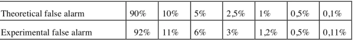
On the whole set of tested background signals, the estimated values for N (from (8)) range approximately from 1.7 to 2.6 with a mean value close to 2. Thus, the number of degrees of freedom of the χ2,N distribution was set to N = 2 and, using the Kolmogorov-Smirnov goodness-of-fit test [21], the likelihood of the χ2,2 hypothesis was verified. A comparison of theoretical and experimental false alarm probabilities obtained on simulated signals without transients (resp. with transients) is reported in table I (resp. table II). It points out that the false alarm probability can be reasonably adjusted to a given value.

Experiments were also performed on real signals sampled at 200 Hz and collected from scalp electrodes (according to the International 10-20 setting) over a 10 min. period of time. The results obtained by automatic detection were compared with those obtained from a visual analysis by a physician who numbered 982 useful waves for the whole period of time. Hypotheses on the law, the degree of freedom of the T_n's and the statistical distribution of G_k's were also verified on short stationary signals segments ; these hypotheses were assessed on a large number of cases (figure 4). The

thresholds λ₁ and λ₂ were adaptively adjusted using the relations described in § IV.1.1 and § IV.1.2. The analysis of the performances (table III) has shown that :

• A large number of useful waves (862 on the 982 extracted by the physician, i.e. 88%) and artifacts were correctly detected by the first detector level, as well as 46 pathological transients (i.e. 5%) considered as non significant because of no interest for diagnosis. Any wave that did not belong to these groups was never exhibited.

• The second level detector rejected a large number of artifact transients (147 on 206 i.e. 68%) and only a small number of useful waves (22 on 982 i.e. 2.5 %) were classified as artifacts.

• The decision structure leads to the detection of low amplitude epileptic events (this result is important since these events have a strong medical significance).

• The introduction of the spatial dimension could improve the current performances : a non detection on one channel often occurs simultaneously with a detection on a close electrode.

A temporal segment extracted from the same data has been used to exemplify the 3-D mapping. The head morphology was described by a CT image volume consisting of 150 slices with a 256x256 spatial resolution. The electrode registration was performed by pointing the inion and the nasion: theses landmarks being known, the location of the sensors can be computed by projecting the standard setting onto the head surface. The interpolation has been carried out by means of spherical splines that provide a good compromise between accuracy and computation time. All these procedures were implemented on a HP 9000-835 computer using the Multipurpose Ray Tracing software [22].

Figures 5 and 6 illustrate the display modes. Any point of view of the head can be selected and a time sequence of potential mapping can be analyzed (figure 5). A sequence of time indexed maps, for the same viewpoint, can also be visualized (figure 6). The two first rows show the original EEG cartography and the two last the module of the 10th level (with to k = 2, f_o = 0,01 a = 1/3) resulting from the wavelet decomposition at the same instants. The interpretation of these data points out that the spike originates in the frontal part of the brain and propagates toward the left temporal region. The raw signal map leads to the same conclusion but a more extended area with both left and right distributions seems involved. This example emphasizes that the wavelet representation provides a better spatial discrimination and has a good sensitivity to the spatio-temporal evolutions. Other experiments on surface and depth recordings show that the changes in the frequency contents observed in epilepsy (recruiting rhythms or spike bursts) can also be separated at a given level of the multiscale decomposition.

VII. CONCLUSION

The presentation of a multi-level structure - based on the time-scale representation and developed to detect fast transients signals which sign an epileptic activity in the electroencephalograph signals - has been described. The search of transients in an observation period was classically brought back to a succession of choices between two hypotheses (presence or absence of spike-like signal). The difficulties come from the fact that the waveforms are changing, that the occurrence law of the events is not known and that the noise added to the signal is non stationary. The tests performed on

simulated and real signals demonstrated that the approach used to adjust the decision thresholds is efficient. These results open new prospects in EEG signal processing : a better detection is obtained in the case of surface signals by using the decomposition levels ; a decision statistics can be built and their properties controlled from the wavelets transform. In addition, a solution has been proposed to fuse morphological and functional features. This 3-D mapping leads to more realistic views of spatio-temporal relationships. It can be applied to the most important episodes automatically extracted from the long term recording, either to the original signals or their transforms. New cues in the localization and the propagation of spikes within the brain can then be expected.

Acknowledgments : The authors are gratful to Pr. J.L. Coatrieux for his suggestions and comments on this paper and to all

the members of the "Unité d'épileptologie Vincent VanGogh"

REFERENCES

[1] Coatrieux. J.L, C. Toumoulin, C. Hamon, L.M. Luo : “Future Trends in 3D Medical Imaging”, IEEE Eng. Med. Biol Magazine, Dec. 1990, pp. 33-39.

[2] Gotman. J : "Computer analysis of the EEG in Epilepsy", In : Handbook of Electroencephalography and Clinical Neurophysiology (Revised Series), Vol. 2 Clinical Applications of Computer Analysis of EEG and other Neurophysiological Signals, edited by F.H. Lopes da Silva, W. Storm van Leeuwen and A. Rémond Amsterdam : Elsevier, 1985 pp. 171-204

[3] Glove. R.J, N. Raghavam, P.Y. Ktonas, J.D. Frost : "Context-based automated detection of epileptogene sharp transient in the EEG : elimination of false positives", IEEE Trans. BME., Vol. 36, pp. 519-527, 1989.

[4] Gotman. J, L.Y. Wang, "State-dependent spike detection : concepts and preliminary results", Electroenceph. Clin. Neurophysiol., Vol. 79, pp. 11-19, 1991.

[5] Dingle. A.A, R.D. Jones, G.J. Carroll, W.R. Fright : "A multistage system to detect epileptiform activity in the EEG", IEEE Trans. BME. Vol. 40, pp. 1260-1268, 1993.

[6] Grossmann. A, J. Morlet : "Decomposition of Hardy functions into square integrable wavelets of constant shape", SIAM. J. Math Anal., Vol. 15, pp. 723-736, 1984.

[7] Daubechies. I : "Orthonormal bases of compactly supported wavelets", Com. Pure Appl. Math., Vol. 41, pp. 909-996, 1988.

[8] Mallat. S.G :

"

[9] Weiss. L.G : "Wavelets and wideband correlation processing", IEEE Signal Proc. Magazine, Vol. 11, pp. 13-32, 1994. [10] Senhadji. L : "Approche multirésolution pour l'analyse des signaux non stationnaires", Thèse de Doctorat de l'Université de Rennes I, Feb. 1993.

[11] Arques. P.Y : "Décisions en traitement du signal", Collection CNET/ENST, Masson, 1979.

[12] Senhadji. L, G. Carrault, J.J. Bellanger : "Détection et cartographie multiéchelles", Progress in Wavelet Analysis and Applications. Y.Meyer & S. Roques Eds. Frontiers, pp. 609-614, 1993.

[13] Dillenseger. J.L, J.L. Coatrieux : "Functional and Morphological Data Fusion in Electroencephalography", Proc. 14th IEEE-EMBS Conf. , Paris, pp. 2022-2023, Nov. 1992.

[14] Jasper. H.H : "Report of the Committee on Methods of Clinical Examinations in Electroencephalography", Electroenceph. and Clinic. Neurophys., Vol. 10, pp. 370-375, 1958.

[15] Perrin. F, J. Pernier, O. Bertrand, J.F. Echallier : "Spherical Splines for Scalp Potential and Current Density Mapping", Electroenceph. and Clinic. Neurophys., Vol. 72, pp. 184-187, 1989.

[16] Nielson. G.M, T.A. Foley, B. Hamann, D. Lane : "Visualizing and Modeling Scattered Multivariate Data", IEEE Comp. Graph. & Appl., Vol. 11, pp. 47-55, 1991.

[17] Siregar. P : "Imagerie fonctionnelle électrique du cerveau et modèles de connaissance quantitatifs et qualitatifs. Propositions pour une approche intégrée", Thèse de Doctorat de l'Université de Rennes I, March 1992.

[18] Coatrieux. J.L, C. Barillot : "A Survey of 3D Display Techniques to Render medical Data", Adv. Res. Works. on 3-D Imaging in Medicine, NATO ASI, vol. F60, Springer Verlag, pp.175-195, June 1990.

[19] Dillenseger. J.L, C. Hamitouche, J.L. Coatrieux : "An Integrated Multi-Purpose Ray Tracing Framework for the Visualization of Medical Images", Proc. 13th. IEEE-EMBS Conf. Orlando, pp. 1125-1126, Nov. 1991.

[20] Dillenseger. J.L : "Imagerie tridimensionnelle morphologique et fonctionnelle en multimodalité", Thèse de Doctorat de l'Université François Rabelais de Touts, Dec. 1992.

[21] Ventsel. H : "Théorie des probabilités", MIR (Ed), Moscou, 1973.

[22] Dillenseger J.L, C. Rocha, J.L. Coatrieux, "'X-Image 3D' : An Evolutionary Software System for Interactive Visualization and Analysis of Multidimensional Biomedical Data", 12th International Congress on Medical Informatics (MIE-94), Lisbon, May 1994.

CAPTIONS

Table I : Estimation of the false alarm rate provided by (6), when no transients are present in the signal, for a given theoretical threshold.

Table II : Estimation of the false alarm rate provided by (6), when transients are added to the signal, for a given theoretical threshold.

Table III : Overall performances of the proposed detector.

Figure 1 : Examples of four EEG periods (10 seconds each). a) Two different types of artifacts, b) and c) Two sorts of background activity exhibiting spikes and transient artifacts, d) A period of background activity (alpha rhythm) without any transient.

Figure 2 : Spikes detection framework based on wavelet transform.

Figure 3 : Example of two EEG channels and the corresponding square modulus of the wavelet transform. Low frequency components are identified at coarse scale (rows a and b), the transient signals are enhanced while the background activities (high frequency noise and Alpha rhythm) are strongly reduced (rows c and d).

Figure 4 : (1) Histogram of T_k, for a real signal with no transients. (2) Histogram of the statistics G_k, for real signals.

Figure 5 : 3D anatomical EEG maps. Different points of view at the same time. Notice the bivariate color scale used for the representation.

Figure 6 : Temporal sequence of :

(1) the original EEG signal (on the first two rows) ;

(2) the module of the 10th level resulting from the wavelet decomposition (k = 2, f_o = 0,01, a = 1/3) at the same instants (two last rows).

-200 -150 -100 -50 0 -30 -20 -10 0 10 20 30 40 50 60 -30 -20 -10 0 10 20 30 -40 -20 0 20 40 60 Spikes Artifacts a) b) c) d)

2

2

2

2

1

λ

2

λ

EEG Signal

Σ

D

_a1

D

D

_a3

D

_a2

n

n

n

n

M

a

Non linear

Transform

Composition

through scales

T

_n

k

_Artifact

Event

Presence of Transient

Background

Signal

Theoretical false alarm 90% 10% 5% 2,5% 1% 0,5% 0,1% Experimental false alarm 92% 11% 6% 3% 1,2% 0,5% 0,11%

Table I

Theoretical false alarm 5% 1% 0,5% 0,1% Experimental false alarm 4,4% 0,9% 0,43% 0,07%

Table II

Non Detection False Alarm Good Detection

First stage 12% 22% 88%

Second stage 14% 7% 86%

0 50 100 150 200 250 0 500 1000 1500 2000 2500 0 50 100 150 200 250 7,1 7,3 7,5 7,7 7,9 8,1 8,3 8,5 (1) (2) Figure 4