HAL Id: hal-01301829
https://hal.archives-ouvertes.fr/hal-01301829
Submitted on 13 Apr 2016
HAL is a multi-disciplinary open access
archive for the deposit and dissemination of
sci-entific research documents, whether they are
pub-lished or not. The documents may come from
teaching and research institutions in France or
abroad, or from public or private research centers.
L’archive ouverte pluridisciplinaire HAL, est
destinée au dépôt et à la diffusion de documents
scientifiques de niveau recherche, publiés ou non,
émanant des établissements d’enseignement et de
recherche français ou étrangers, des laboratoires
publics ou privés.
Portfolios of Subgraph Isomorphism Algorithms
Lars Kotthoff, Ciaran Mccreesh, Christine Solnon
To cite this version:
Lars Kotthoff, Ciaran Mccreesh, Christine Solnon. Portfolios of Subgraph Isomorphism Algorithms.
10th International Conference on Learning and Intelligent OptimizatioN Conference (LION), May
2016, Ischia Island (Naples), Italy. pp.107-122. �hal-01301829�
Portfolios of Subgraph Isomorphism Algorithms
Lars Kotthoff?1, Ciaran McCreesh??2, and Christine Solnon? ? ?3
1
University of British Columbia, Vancouver, Canada 2
University of Glasgow, Glasgow, Scotland 3
INSA-Lyon, LIRIS, UMR5205, F-69621, France
Abstract. Subgraph isomorphism is a computationally challenging problem with important practical applications, for example in computer vision, biochemistry, and model checking. There are a number of state-of-the-art algorithms for solving the problem, each of which has its own performance characteristics. As with many other hard problems, the single best choice of algorithm overall is rarely the best algorithm on an instance-by-instance. We develop an algorithm selection approach which leverages novel features to characterise subgraph isomorphism problems and dynamically decides which algorithm to use on a per-instance basis. We demonstrate substantial performance improvements on a large set of hard benchmark problems. In addition, we show how algorithm selection models can be leveraged to gain new insights into what affects the performance of an algorithm.
1
Introduction
The subgraph isomorphism problem is to find an adjacency-preserving injective mapping from vertices of a small pattern graph to vertices of a large target graph. This NP-complete problem has many important practical applications, for example in computer vision [6, 25], biochemistry [8], and model checking [24]. There exist various exact algorithms, which have been compared on a large suite of instances by McCreesh and Prosser [15]. These experiments indicated that the single best algorithm depends on the CPU time limit considered: for very small time limits, VF2[5] is the best choice, whereas the GLASGOWalgorithm [15] has better success rates for larger time limits. They also showed that on an instance by instance basis, other algorithms are often better. The per-instance algorithm selection problem [21] is to select from an algorithm portfolio [9, 10] the algorithm expected to perform best on a given problem instance. Algorithm selection systems usually build machine learning models of the algorithms or the portfolio which they are contained in to forecast which algorithm to use in a particular context. Using the predictions, one or more algorithms from the portfolio can be selected to be run sequentially or in parallel.
In our subgraph isomorphism context, algorithm performance is highly constrained by memory bandwidth (as pointed out by Sabharwal and Samulowitz [22] for SAT
?
This work was supported by an NSERC E.W.R. Steacie Fellowship and under the NSERC Discovery Grant Program.
??This work was supported by the Engineering and Physical Sciences Research Council [grant number EP/K503058/1]
? ? ?
solvers). Therefore, we cannot simply run different algorithms in parallel, and we consider the case where exactly one algorithm is selected for solving the problem. One of the most prominent and successful systems that employs this approach is SATzilla [28], which defined the state of the art in SAT solving for a number of years. Other application areas include constraint solving [19], the travelling salesperson problem [13], and AI planning [23]. The interested reader is referred to a recent survey [12] for additional information on algorithm selection.
Overview of the paper. We formally define the subgraph isomorphism problem in Section 2. In Section 3, we describe the main existing algorithms for solving this problem, and we also introduce two new algorithms which are derived from Solnon’s LAD algorithm [26]. In Section 4, we experimentally compare eight state-of-the-art algorithms. We introduce a large benchmark set composed of 5725 instances grouped into twelve classes. Ten of these classes were considered in the experimental study reported by McCreesh and Prosser [15]; two are new. We evaluate the algorithms on this benchmark set, and show that they have very complementary performance. In particular, we show that depending on the CPU time limit, different algorithms achieve the best performance on the entire benchmark set. In Section 5, we discuss the features that are used to describe instances, and we describe our algorithm selection approach. It combines a presolving step, which allows us to easy instances very quickly, with an algorithm selection step that uses LLAMA[11]. In Section 6, we experimentally evaluate our selection approach and show that it is able to close more than 60 % of the gap between the single best and the virtual best solver. We conclude and give directions for future work in Section 7.
2
Definitions and Notations
A graph G = (N, E) consists of a node set N and an edge set E ⊆ N × N , where an edge (u, u0) is a pair of nodes. The number of neighbors of a node u is called the degree of u, denoted d◦(u) = #{(u, u0) ∈ E}. In this paper, we implicitly consider non-directed graphs, such that (u, u0) ∈ E ⇔ (u0, u) ∈ E. The extension to directed graphs is rather straightforward, and all algorithms compared in this paper can handle directed graphs as well.
Given a pattern graph Gp = (Np, Ep) and a target graph Gt = (Nt, Et), the
subgraph isomorphism problemconsists of deciding whether Gpis isomorphic to some
subgraph of Gt. More formally, the goal is to find an injective matching f : Np→ Nt,
that associates a different target node to each pattern node, and preserves pattern edges, i.e. ∀(u, u0) ∈ Ep, (f (u), f (u0)) ∈ Et. Note that the subgraph is not necessarily induced,
so that two pattern nodes not linked by an edge may be mapped to two target nodes which are linked by an edge. We define np = #Np, nt= #Nt, ep= #Ep, et= #Et,
and dpand dtto be the maximum degrees of the graphs Gpand Gt.
3
Subgraph Isomorphism Algorithms
Subgraph isomorphism problems may be solved by a systematic exploration of the search space consisting of all possible injective matchings from Np to Nt: starting
from an empty matching, one incrementally extends a partial matching by matching a non-matched pattern node to a non-matched target node until either some edges are not matched by the current matching (so the search must backtrack to a previous choice point and go on with another extension), or all pattern nodes have been matched (a solution has been found). To reduce the search space, this exhaustive exploration is combined with filtering techniques that aim at removing candidate pairs of non-matched pattern-target nodes (u, v) ∈ Np× Nt. Different filtering techniques may be considered;
some are stronger than others (they remove more candidate pairs), but also have higher time complexities.
3.1 Filtering for Subgraph Isomorphism
The simplest form of filtering is to propagate difference constraints (which ensure that the matching is injective) and edge constraints (which ensure that the matching preserves pattern edges): each time a pattern node u ∈ Npis matched with a target node v ∈ Nt,
one removes every candidate pair (u0, v0) ∈ Np× Ntsuch that either v0 = v (difference
constraint) or (u, u0) is a pattern edge but (v, v0) is not a target edge (edge constraint). This simple filtering (called Forward-Checking) is very fast to achieve: in O(np) for
difference constraints, and in O(dp· nt) for edge constraints. It is used, for example, in
McGregor’s algorithm [17] and in VF2[5].
R´egin [20] introduced a stronger filtering for difference constraints, which ensures that all pattern nodes can be matched with different target nodes, all together. This filtering (called All-Different Generalized Arc Consistency) removes more candidate pairs than when each difference constraint is propagated separately which Forward-Checking. However, it is also more time consuming as it requires O(n2
p· n2t) time.
Various filtering techniques have been tried for edge constraints. Ullman [27] in-troduced a filtering which ensures that for each pattern edge (u, u0) ∈ Ep and each
candidate pair (u, v) ∈ Np× Nt, there exists a candidate pair (u0, v0) ∈ Np × Nt
such that (v, v0) is a target edge. Candidate pairs (u, v) that do not satisfy this property are iteratively removed until a fixed point is reached. This filtering (called Arc Consis-tency) removes more candidate pairs than Forward-Checking, but it is also more time consuming as it runs in O(ep· n2t) when using AC4 [18].
Stronger filtering may be obtained by propagating edge constraints in a more global way, as proposed by Larrosa and Valiente [14]. The idea is to check for each candidate pair (u, v) ∈ Np× Ntthat the number of pattern nodes adjacent to u is smaller than
or equal to the number of target nodes that are both adjacent to v and that may be matched with nodes adjacent to u. This is done in O(n2p· n2t). This idea was generalised
by Solnon’s LADalgorithm [26], where, for each candidate pair (u, v) ∈ Np× Nt,
a redundant Local All-Different constraint ensures that each neighbour of u may be matched with a different neighbour of v. This is done in O(np· nt· d2p· d2t).
3.2 Propagation of Invariant Properties
Some filtering techniques exploit invariant properties, i.e. properties associated with nodes such that nodes may be matched only if they have compatible properties. A classical property is the degree: a pattern node u ∈ Npmay be matched with a target
node v ∈ Ntonly if d◦(u) ≤ d◦(v). This property is usually used at the beginning of
the search to reduce the set of candidate pairs to {(u, v) ∈ Np× Nt| d◦(u) ≤ d◦(v)}.
Other examples of invariant properties are the number of cycles of length k passing through the node, and the number of cliques of size k containing the node, which must be smaller for a pattern node than for its matched target node. Invariant properties may also be associated with pairs of nodes. For example, the number of paths of length k between two pattern nodes is smaller than or equal to the number of paths of length k between the target nodes with which they may be matched. These invariant properties are used, for example,
– by Battiti and Mascia [2], to remove candidate pairs (u, v) ∈ Np× Ntsuch that the
number of paths starting from pattern node u is greater than the number of paths starting from target node v;
– by Audemard et al. [1] to generalise the locally all-different constraint proposed by Solnon [26] so that it ensures that a subset of pattern nodes can be matched with all different compatible target nodes, where compatibility is defined with respect to invariant properties;
– by McCreesh and Prosser [15] to filter the set of candidate pairs before starting the search, and to generate additional implied adjacency-like constraints which are processed during search.
Audemard et al. [1] do not limit the length of paths considered, and iteratively increment the length until no more pairs are removed. Battiti and Mascia [2], and McCreesh and Prosser [15] parameterise their algorithms by the maximum path length considered when counting paths: larger values for this parameter remove more candidate pairs, but are also more time consuming. Battiti and Mascia’s experiments show that the best setting depends on the instance considered, and that a portfolio running several randomised versions in time-sharing decreases the total CPU time needed to find a solution for feasible instances. McCreesh and Prosser simply set the parameter to 3, as this setting presented the best overall performance in their case.
4
Experimental Comparison of Individual Algorithms
We consider six algorithms from the literature and propose two novel ones.
4.1 Algorithms from the Literature
We selected the following algorithms from the literature, based on their performance. – VF2 [5] performs weak filtering that is especially fast on trivially satisfiable
in-stances;
– LAD[26] combines two strong but expensive filtering techniques (All-Different Generalized Arc Consistency and Locally All-Different);
– GLASGOW[15] does expensive preprocessing based on path length invariant prop-erties to generate additional constraints, followed by weaker filtering (forward-checking, and a heuristic All-Different propagator which can miss deletions) and conflict-directed backjumping during search.
We have not considered the algorithm introduced in [29] because it is outperformed by LAD. Also, we have not considered MIP nor SAT solvers because they are not competitive with the selected algorithms [16].
The GLASGOWalgorithm has a parameter, which controls the lengths of paths used when reasoning about non-adjacent vertices. In experiments reported by McCreesh and Prosser [15], the choice of paths of length 3 was used as a reasonable compromise— longer paths lead to prohibitively expensive preprocessing on larger, denser instances. This is often not the best choice on an instance by instance basis: sometimes path-based reasoning gives no benefit at all, sometimes considering only paths of length 2 suffices, occasionally paths of length 4 are helpful, and even looking at paths of length 3 is relatively expensive on some graphs. We thus consider all lengths up to 4, naming these variants GLASGOW1through GLASGOW4.
4.2 New Algorithms
We introduce two new variants of LAD. The first, called INCOMPLETELAD, does weaker filtering which is applied once, without performing a backtracking search, and very quickly detects inconsistencies on many instances: for each pattern node u, we check if there exists at least one target node v such that for each neighbor u0of u there exists a different neighbor v0 of v such that the degree of u0 is smaller than or equal to the degree of v0. INCOMPLETELADis an incomplete algorithm that checks a sufficient, but not necessary, condition for inconsistency: when it does not detect inconsistency, the instance may still be unsatisfiable. Its main benefit is that it runs very fast: its time complexity is O(np(nt+ et)).
The second variant of LADis called PATHLAD. It combines the locally all-different constraints introduced by Solnon [26] with the exploitation of path length properties proposed by Audemard et al. [1]. The idea is to label each edge (u, v) with the number of paths of length 2 between u and v, and each node u with the number of cycles of length 3 passing through u, and to add the constraint that the label of a pattern node (resp. edge) must be smaller than or equal to the label of its associated target node (resp. edge).
4.3 Problem Instances
We consider a large benchmark set of 5725 instances, which are available in a simple text format4. These instances are grouped into 12 classes.
– Class 1 contains randomly generated scale-free graphs [29].
– Classes 2 and 3 contain instances built from a database containing various kinds of graph gathered by Larrosa and Valiente [14]: class 2 contains small instances generated from the first 50 graphs of the database, and class 3 contains larger instances with pattern graphs from the first 50 graphs of the database and target graphs from the next 50 graphs.
– Classes 4 to 8 contain randomly generated graphs from a database of graphs com-monly used for benchmarking subgraph isomorphism algorithms [7]: bounded-degree graphs for classes 4 and 5, regular meshes for classes 6 and 7, and random graphs with uniform edge probabilities for class 8. All of these instances are satisfi-able.
– Classes 9 and 10 contain instances from segmented images [6, 25]. – Class 11 contains instances from meshes modeling 3D objects [6].
– Class 12 contains random graph instances chosen to be close to the satisfiable-unsatisfiable phase transition—these instances are expected to be particularly chal-lenging, despite their small size.
Note that Classes 3 and 12 were not considered in the previous experimental study by McCreesh and Prosser [15]. Our set of instances is much larger than that of Battiti and Mascia [2], who were the first to propose algorithm portfolios for subgraph isomorphism problems. Battiti and Mascia only considered a pure parallel portfolio consisting of two randomised solvers without a selection mechanism. Their problem set consisted entirely of satisfiable instances.
4.4 Experimental Setup
We measured runtimes on machines with Intel Xeon E5-2640 v2 CPUs and 64GBytes RAM, running Scientific Linux 6.5. We used the C++ implementation of the GLASGOW algorithm [15], the C implementation of LAD[26], and the VFLib C++ implementation of VF2[5]. Software was compiled using GCC 4.9. Each problem instance was run with a timeout of 108milliseconds (≈ 27.8 hours).
4.5 Results
Figure 1 displays the evolution of the cumulative number of instances solved with respect to CPU time. It shows us that the best solver depends on the time limit considered. INCOMPLETELADis able to solve easy unsatisfiable instances very quickly, in a few milliseconds. For time limits less than 5 ms, it is the best solver. However, it is not able to solve harder unsatisfiable instances, nor can it solve satisfiable instances.
PATHLADand GLASGOW1outperform INCOMPLETELADfor longer time limits: PATHLADis the best solver for time limits greater than 5 ms and less than 40 ms, and GLASGOW1is the best solver for time limits greater than 40 ms and less than 3000 ms. GLASGOW2becomes the best solver for time limits greater than 3000 ms. As we increase the CPU time limit, the performance of variants of GLASGOWwith longer paths (GLASGOW3and GLASGOW4) improves. This is what we expect, as more reasoning is expensive, but increases the potential reduction of the search space. Eventually, GLASGOW2and GLASGOW3become very closely matched, and with runtimes very close to the limit, GLASGOW4nearly catches up. This behavior is class-dependent: for class 2, for example, the behavior is roughly monotone, with GLASGOW1dominating for low runtimes, then GLASGOW2, then GLASGOW3, then GLASGOW4each becoming best as the runtimes increase.
The figure illustrates the potential for portfolios and algorithm selection we have: there is clearly no single solver that dominates throughout.
5725 0 1000 2000 3000 4000 5000 100 101 102 103 104 105 106 107 108 Cumulati v e Number of Instances Solv ed Runtime (ms) INCOMPLETELAD VF2 LAD GLASGOW4 PATHLAD GLASGOW1 GLASGOW2 GLASGOW3 VBS
Fig. 1. Cumulative number of solved instances over CPU time for the eight algorithms we consider in this paper, and the virtual best solver (VBS) that shows the best solver on an instance by instance basis.
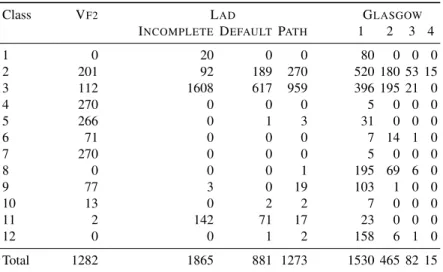
Class VF2 LAD GLASGOW
INCOMPLETE DEFAULT PATH 1 2 3 4
1 0 20 0 0 80 0 0 0 2 201 92 189 270 520 180 53 15 3 112 1608 617 959 396 195 21 0 4 270 0 0 0 5 0 0 0 5 266 0 1 3 31 0 0 0 6 71 0 0 0 7 14 1 0 7 270 0 0 0 5 0 0 0 8 0 0 0 1 195 69 6 0 9 77 3 0 19 103 1 0 0 10 13 0 2 2 7 0 0 0 11 2 142 71 17 23 0 0 0 12 0 0 1 2 158 6 1 0 Total 1282 1865 881 1273 1530 465 82 15 Table 1. Number of times each algorithm is best, for each class.
Furthermore, the virtual best solver (VBS), which considers the best algorithm for each instance separately, obtains much better results, showing us that the algorithms have complementary performance. The difference between VBS and single best is particularly pronounced for CPU time limits less than 1000 ms. In many applications, it is important to have the fastest possible algorithm even if the absolute differences in CPU time are small. For example, in pattern recognition [6, 25] and chemical [8] applications, we often have to solve the subgraph isomorphism problem repeatedly for a very large number of graphs (in order to find a pattern image or molecule in a large database of target images or compounds, for example), so having an algorithm that is able to solve an instance in 100 ms instead of 1000 ms makes a big difference. Therefore, it is important to select the best algorithm for each instance, even if the instance is an easy one. Furthermore, this selection process should not unduly penalise easy instances, i.e. it should not take more time than the solution process time for these instances.
Table 1 shows us that we cannot simply select algorithms based on the instance class. For all classes, there are always at least two algorithms which are the best for at least one instance of the class. In particular, for classes 2 and 3, each algorithm is the best for at least one instance (except GLASGOW4for class 3).
5
Algorithm Selection Approach
Our approach is composed of three steps. First, we run two presolvers in a static way to quickly solve easy instances. This ensures that we achieve good performance on instances that can be solved in a small amount of time. Second, we extract features from instances which are not solved by the first step. Finally, we run algorithm selection to choose the algorithm to solve the instance with.
5.1 Presolving
Experimental results reported in Section 4.5 show that INCOMPLETELADis very fast (7 ms on average) and able to solve 1919 instances from our benchmark set very quickly. Therefore, we first run INCOMPLETELAD: if unsatisfiability is detected, we do not need to process it further.
VF2is also able to solve many easy instances very quickly: from the 3806 instances that are not solved by INCOMPLETELAD, 1470 are solved by VF2 in less than 50 milliseconds. Therefore, after running INCOMPLETELAD, we run the VF2solver for 50 ms. This solves easy instances without the overhead of running algorithm selection and avoids potentially making incorrect solver choices.
We also include VF2in the portfolio, as it may solve an instance given more time, but not INCOMPLETELAD, as it is an incomplete solver that cannot solve satisfiable instances.
After the presolving step, we are left with 2336 hard instances that we consider for algorithm selection.
5.2 Feature Extraction
If presolving does not give us a solution, we extract features that characterize the instances. For both the pattern and the target graph, we consider some basic graph properties that can be computed very quickly:
– the number of vertices and edges;
– the density—we expect that some kinds of filtering (like those based upon locally all-different constraints) might be expensive and ineffective on dense graphs; – how many loops (self-adjacent vertices) the graph contains—as loops must be
mapped to loops, this could have a strong effect on how easy an instance is; – the mean and maximum degrees, and whether or not every vertex has the same
degree (the degree-based invariants used by LADand GLASGOWdo nothing at the top of search if every vertex has the same degree);
– whether or not the graph is connected;
– the mean and maximum distances between all pairs of vertices (if nearly all vertices are close together, path-based reasoning is likely to be ineffective) and the proportion of vertex pairs which are at least 2, 3 and 4 apart.
Alongside these basic features, we include information computed by INCOMPLETELAD. To (try to) prove inconsistency, INCOMPLETELADremoves candidate pairs. The number of successfully removed pairs gives information on the distribution of edges (the fewer removed pairs, the more uniform the distribution). As well as the number of removed pairs, we also record the percentage with respect to all possible pairs, and the minimum and maximum percentages of removed values on a per-variable basis. Finally, we include the CPU time required to compute these features as features. However, those features were not more informative than the other ones.
5.3 Selection Model
We use LLAMA[11] to build our algorithm selection model. LLAMAsupports the most common algorithm selection approaches used in the literature. We performed a set of preliminary experiments to determine the approach that works best here.
We use 10-fold cross-validation to determine the performance of the LLAMAmodels. The entire set of instances was randomly partitioned into 10 subsets of approximately equal size. Of the 10 subsets, 9 were combined to form the training set for the algorithm selection models, which were evaluated on the remaining subset. This process was repeated 10 times for all possible combinations of training and test sets. At the end of this process, each problem instance in the original set was used exactly once to evaluate the performance of the algorithm selection models.
LLAMA’s pairwise regression approach with random forest regression gave the best performance. The idea is very similar to the pairwise classification models used by Xu et al. [28]. For each pair of algorithms in our portfolio, we train a model that predicts the performance difference between them. If the first algorithm is better than the second, the difference is positive, otherwise negative. The algorithm with the highest cumulative performance difference, i.e. the most positive difference over all other algorithms, is chosen to be run.
As this approach gives very good performance already, we did not tune the parameters of the random forest machine learning algorithm. It is possible that overall performance can be improved by doing so and we make no claims that the particular algorithm selection approach we use in this paper cannot be improved.
The data we use in this paper is available as ASlib [3] scenario GRAPHS-2015.
6
Experimental Evaluation of Algorithm Selection
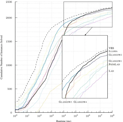
Table 2 shows the performance of our algorithm selection approach, compared to two baselines, on the set of 2336 hard instances. The virtual best solver is the oracle predictor that, for each instance, chooses the best solver from our portfolio. This is the upper bound of what an algorithm selection approach can achieve. The single best solver is the one solver from the portfolio that has the overall best performance across the entire set of instances, at the CPU time limit of 108ms, i.e. GLASGOW2. We consider it a lower bound on the performance of the algorithm selection approach. We are able to solve 30 more instances than the single best solver within the timeout, with only an additional 16 to the virtual best. In terms of average performance, we are able to close 64 % of the gap between the single best and the virtual best solver.
Figure 2 shows the cumulative number of solved instances over time for the individual solvers, the virtual best solver, and the LLAMA algorithm selection approach. The algorithm selection model does not perform well for instances that can be solved quickly because of the overhead incurred through feature computation. As the instances become more difficult to solve, its performance improves.
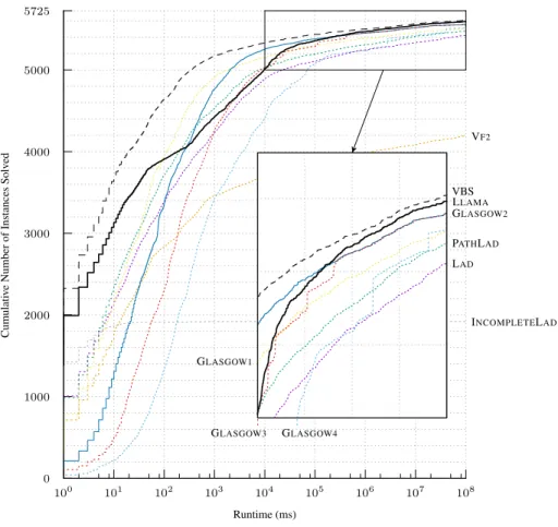
Table 2 shows the performance of the selection model on its own. The performance of the entire algorithm selection system, including the preprocessing, is shown in Table 3. Our system is able to close more than 60 % of the gap between single and virtual best, similar to the results on the set of hard instances.
Figure 3 shows the cumulative number of solved instances over time for the algorithm selection system including INCOMPLETELADand VF2 presolving on the full set of instances. The performance on small instances is much better than the LLAMAselector alone (cf. Figure 2) and the region where LLAMAperforms worse than the individual solvers is now limited to approximately 102to 105milliseconds.
We train the algorithm selection model specifically for the timeout of 108
millisec-onds. In particular, we are interested in minimising the performance difference to the virtual best. Problem instances that take longer to solve contribute more to this difference than easy instances and therefore carry more weight for the algorithm selection model. That is, choosing the wrong solver for a hard instances is much worse than choosing the wrong solver for an easy instance.
Figures 2 and 3 show that for the easy instances from the set of hard instances, the performance improvement through algorithm selection is negated by the cost of computing the features. The presolving steps improve performance dramatically over the full set of instances (cf. Tables 2 and 3).
6.1 Analysis of Features Used by the Model
model mean MCP solved instances mean performance virtual best 0 2219 5822809 LLAMA 705097 2203 6529563
GLASGOW2 1960683 2173 7783492
Table 2. Algorithm selection performance on the set of 2336 hard instances. MCP is the misclas-sification penalty; that is, the additional time required to solve an instance because of choosing solvers that perform worse than the best. Mean MCP and performance are over all 2336 instances; when an instance is not solved, its performance is set to the time limit (108ms).
2336 0 500 1000 1500 2000 100 101 102 103 104 105 106 107 108 Cumulati v e Number of Instances Solv ed Runtime (ms) GLASGOW3 GLASGOW4 LAD PATHLAD GLASGOW1 GLASGOW2 VBS LLAMA
Fig. 2. Cumulative number of solved instances over time for the virtual best solver, LLAMA, and the single best solver GLASGOW2on the set of 2336 hard instances. Other individual solvers are shown as dotted lines, in the same colors as Figure 1.
model mean MCP solved instances mean performance virtual best 0 5608 2375913 LLAMA 287704 5592 2664293
GLASGOW2 798660 5562 3174573
Table 3. Algorithm selection system performance on the full set of 5725 instances.
5725 0 1000 2000 3000 4000 5000 100 101 102 103 104 105 106 107 108 Cumulati v e Number of Instances Solv ed Runtime (ms) INCOMPLETELAD VF2 GLASGOW3 GLASGOW4 LAD PATHLAD GLASGOW1 GLASGOW2 VBS LLAMA
Fig. 3. Cumulative number of solved instances over time for the virtual best solver, LLAMA, and the single best solver GLASGOW2on the full set of 5725 instances. Other individual solvers are shown as dotted lines, in the same colors as Figure 1.
– the maximum degree of the pattern graph; – the mean degree of the target graph;
– the proportion of target vertices that are at least distance 3 apart; – the number of values removed during INCOMPLETELADpresolving.
We introduced the proportion of target vertices that are at least 3 apart as a feature expecting it to be helpful in distinguishing between GLASGOWvariants—if few vertices are far apart, longer paths are unlikely to be useful. However, in practice this feature also gives a rough indication of how sparse the graph is—locally all-different filtering is weak and expensive on dense graphs, and the feature turned out to be helpful for selecting between GLASGOWand LADvariants too.
As expected, both the pattern graph and the target graph provide important features. We conclude that even basic graph properties are predictive of sophisticated algorithms’ performance.
6.2 Analysis of PATHLADversus GLASGOW2
To gain further insight into the behavior of the algorithms, we investigated what affects the relative performance of PATHLADand GLASGOW2. This pair is of particular interest because they are the best “medium-case” algorithms that use strong and weak filtering during search, respectively. We used machine learning techniques (JRip [4]) to train a simple, human-understandable model which is able to distinguish these solvers for the 2336 hard instances and gives performance better than always choosing one of them. The model uses four rules:
1. If INCOMPLETELADpresolving removes at least 28.01 % of the pairs, and at least 94.12 % of the values from at least one domain, then pick PATHLAD.
2. If the target has at least 610 vertices, and if the maximum distance between any two pattern vertices is at most 8, and if the pattern is not regular, and if the time taken to compute the distance-based features on the target graph is no more than 1277 ms, then pick PATHLAD.
3. If INCOMPLETELADfiltering removed at least 5.90 % of possible pairs, and if less than 84.66 % of the pattern vertices are within distance 2 of each other, then pick PATHLAD.
4. Otherwise, pick GLASGOW2.
The first and third rules intuitively make sense: if INCOMPLETELADfiltering does well, it is likely that continuing with this kind of filtering during search will be successful. The third rule also excludes using PATHLADon very dense pattern graphs, where locally all-different filtering is expensive and weak. The second rule is less obvious: while PATHLADfiltering is weak on regular graphs and it makes sense to exclude this case, the other components appear to exclude large and dense target graphs. The model suggests that it would be worth exploring dynamically enabling or disabling locally all-different filtering during search, based upon very simple features which could be recomputed as search progresses and conditions change.
This provides an interesting insight into the behavior of our algorithms, as well as giving indications for future work.
7
Conclusion and Future Work
The problem of identifying subgraph isomorphisms is a hard computational problem that has many applications in diverse areas. In this paper, we presented a portfolio of six algorithms from the literature and two new variants of the LADalgorithm. We introduced a set of novel features to characterise subgraph isomorphism problems and leveraged them to select the most appropriate algorithm from the portfolio for each instance.
We demonstrated that our algorithm selection approach achieves substantial perfor-mance improvements over the single algorithm that has the best perforperfor-mance on our benchmark set. We showed that combining an algorithm selection approach with a new incomplete variant of LADthat is able to detect inconsistencies and a presolver boosts performance even further. Finally, we showed how insights from machine learning can guide algorithm development.
Directions for future work include scheduling multiple solvers to run instead of a single one; in particular the GLASGOWalgorithms provide a multi-core parallel imple-mentation, which can use a configurable number of threads. It would also be interesting to investigate other variants of the subgraph isomorphism problem.
References
1. Audemard, G., Lecoutre, C., Modeliar, M.S., Goncalves, G., Porumbel, D.: Scoring-based neighborhood dominance for the subgraph isomorphism problem. In: Principles and Practice of Constraint Programming - 20th International Conference, CP 2014, Lyon, France, Septem-ber 8-12, 2014. Proceedings. pp. 125–141 (2014), http://dx.doi.org/10.1007/ 978-3-319-10428-7_12
2. Battiti, R., Mascia, F.: An algorithm portfolio for the sub-graph isomorphism problem. In: Engineering Stochastic Local Search Algorithms. Designing, Implementing and Analyzing Effective Heuristics, International Workshop, SLS 2007, Brussels, Belgium, September 6-8, 2007, Proceedings. Lecture Notes in Computer Science, vol. 4638, pp. 106–120. Springer (2007)
3. Bischl, B., Kerschke, P., Kotthoff, L., Lindauer, M.T., Malitsky, Y., Fr´echette, A., Hoos, H.H., Hutter, F., Leyton-Brown, K., Tierney, K., Vanschoren, J.: Aslib: A benchmark library for algorithm selection. Artificial Intelligence Journal (2016), in press.
4. Cohen, W.W.: Fast effective rule induction. In: Twelfth International Conference on Machine Learning. pp. 115–123. Morgan Kaufmann (1995)
5. Cordella, L.P., Foggia, P., Sansone, C., Vento, M.: A (sub)graph isomorphism algorithm for matching large graphs. IEEE Trans. Pattern Anal. Mach. Intell. 26(10), 1367–1372 (2004), http://doi.ieeecomputersociety.org/10.1109/TPAMI.2004.75 6. Damiand, G., Solnon, C., de la Higuera, C., Janodet, J.C., Samuel, E.: Polynomial
algo-rithms for subisomorphism of nD open combinatorial maps. Computer Vision and Image Understanding (CVIU) 115(7), 996–1010 (2011)
7. De Santo, M., Foggia, P., Sansone, C., Vento, M.: A large database of graphs and its use for benchmarking graph isomorphism algorithms. Pattern Recogn. Lett. 24(8), 10671079 (May 2003), http://dx.doi.org/10.1016/S0167-8655(02)00253-2
8. Giugno, R., Bonnici, V., Bombieri, N., Pulvirenti, A., Ferro, A., Shasha, D.: Grapes: A software for parallel searching on biological graphs targeting multi-core architectures. PLoS ONE 8(10), e76911 (10 2013), http://dx.doi.org/10.1371%2Fjournal.pone. 0076911
9. Gomes, C.P., Selman, B.: Algorithm portfolios. Artificial Intelligence 126(1-2), 43–62 (2001) 10. Huberman, B.A., Lukose, R.M., Hogg, T.: An economics approach to hard computational
problems. Science 275(5296), 51–54 (1997)
11. Kotthoff, L.: LLAMA: Leveraging learning to automatically manage algorithms. Tech. Rep. arXiv:1306.1031, arXiv (Jun 2013), http://arxiv.org/abs/1306.1031
12. Kotthoff, L.: Algorithm selection for combinatorial search problems: A survey. AI Magazine 35(3), 48–60 (2014)
13. Kotthoff, L., Kerschke, P., Hoos, H., Trautmann, H.: Improving the state of the art in inexact TSP solving using per-instance algorithm selection. In: LION 9 (2015)
14. Larrosa, J., Valiente, G.: Constraint satisfaction algorithms for graph pattern matching. Math-ematical. Structures in Comp. Sci. 12(4), 403–422 (2002)
15. McCreesh, C., Prosser, P.: A parallel, backjumping subgraph isomorphism algorithm using supplemental graphs. In: Pesant, G. (ed.) Principles and Practice of Constraint Programming, Lecture Notes in Computer Science, vol. 9255, pp. 295–312. Springer International Publishing (2015), http://dx.doi.org/10.1007/978-3-319-23219-5_21
16. McCreesh, C., Prosser, P., Trimble, J.: Heuristics and really hard instances for subgraph isomorphism problems. In: IJCAI (2016), to appear
17. McGregor, J.J.: Relational consistency algorithms and their application in finding subgraph and graph isomorphisms. Inf. Sci. 19(3), 229–250 (1979)
18. Mohr, R., Henderson, T.: Arc and path consistency revisited. Artificial Intelligence 28, 225– 233 (1986)
19. O’Mahony, E., Hebrard, E., Holland, A., Nugent, C., O’Sullivan, B.: Using case-based reasoning in an algorithm portfolio for constraint solving. In: Proceedings of the 19th Irish Conference on Artificial Intelligence and Cognitive Science (Jan 2008)
20. R´egin, J.C.: A filtering algorithm for constraints of difference in CSPs. In: Proc. 12th Conf. American Assoc. Artificial Intelligence. vol. 1, pp. 362–367. Amer. Assoc. Artificial Intelli-gence (1994)
21. Rice, J.R.: The algorithm selection problem. Advances in Computers 15, 65–118 (1976) 22. Sabharwal, A., Samulowitz, H.: Principles and Practice of Constraint Programming:
20th International Conference, CP 2014, Lyon, France, September 8-12, 2014. Proceed-ings, chap. Insights into Parallelism with Intensive Knowledge Sharing, pp. 655–671. Springer International Publishing, Cham (2014), http://dx.doi.org/10.1007/ 978-3-319-10428-7_48
23. Seipp, J., Braun, M., Garimort, J., Helmert, M.: Learning portfolios of automatically tuned planners. In: ICAPS (2012)
24. Sevegnani, M., Calder, M.: Bigraphs with sharing. Theoretical Computer Science 577(0), 43 – 73 (2015), http://www.sciencedirect.com/science/article/pii/ S0304397515001085
25. Solnon, C., Damiand, G., de la Higuera, C., Janodet, J.: On the complexity of submap isomorphism and maximum common submap problems. Pattern Recognition 48(2), 302–316 (2015)
26. Solnon, C.: Alldifferent-based filtering for subgraph isomorphism. Artif. Intell. 174(12-13), 850–864 (2010), http://dx.doi.org/10.1016/j.artint.2010.05.002 27. Ullmann, J.R.: An algorithm for subgraph isomorphism. J. ACM 23(1), 31–42 (1976) 28. Xu, L., Hutter, F., Hoos, H.H., Leyton-Brown, K.: SATzilla: Portfolio-based algorithm
selec-tion for SAT. J. Artif. Intell. Res. (JAIR) 32, 565–606 (2008)
29. Zampelli, S., Deville, Y., Solnon, C.: Solving subgraph isomorphism problems with constraint programming. Constraints 15(3), 327–353 (2010)