Comparison of Monte Carlo Methods Efficiency to Solve Radiative Energy Transfer in High Fidelity Unsteady 3D Simulations

HAL Id: hal-01781006

https://hal.archives-ouvertes.fr/hal-01781006

Submitted on 28 Apr 2018

HAL is a multi-disciplinary open access

archive for the deposit and dissemination of

sci-entific research documents, whether they are

pub-lished or not. The documents may come from

teaching and research institutions in France or

abroad, or from public or private research centers.

L’archive ouverte pluridisciplinaire HAL, est

destinée au dépôt et à la diffusion de documents

scientifiques de niveau recherche, publiés ou non,

émanant des établissements d’enseignement et de

recherche français ou étrangers, des laboratoires

publics ou privés.

Comparison of Monte Carlo Methods Efficiency to Solve

Radiative Energy Transfer in High Fidelity Unsteady 3D

Simulations

Lorella Palluotto, Nicolas Dumont, Pedro Rodrigues, Chai Koren, Ronan

Vicquelin, Olivier Gicquel

To cite this version:

Lorella Palluotto, Nicolas Dumont, Pedro Rodrigues, Chai Koren, Ronan Vicquelin, et al.. Comparison

of Monte Carlo Methods Efficiency to Solve Radiative Energy Transfer in High Fidelity Unsteady 3D

Simulations. ASME Turbo Expo 2017: Turbomachinery Technical Conference and Exposition, Jun

2017, Charlotte, North Carolina, United States. �10.1115/GT2017-64179�. �hal-01781006�

COMPARISON OF MONTE CARLO METHODS EFFICIENCY TO SOLVE RADIATIVE

ENERGY TRANSFER IN HIGH FIDELITY UNSTEADY 3D SIMULATIONS

Lorella Palluotto§∗_{, Nicolas Dumont}§_{, Pedro Rodrigues}§_{, Chai Koren}‡§_{, Ronan Vicquelin}§_{, Olivier Gicquel}§ §_{Laboratoire EM2C, CNRS}

CentraleSup ´elec Universit ´e Paris-Saclay Grande Voie des Vignes, 92295 Chatenay-Malabry cedex, France

‡_{Air Liquide}

Centre de Recherche Paris-Saclay 1 Chemin de la Porte des Loges, 78350

Les-Loges-en-Josas, France

ABSTRACT

The present work assesses different Monte Carlo methods in radiative heat transfer problems, in terms of accuracy and computational cost. Achieving a high scalability on numerous CPUs with the conventional forward Monte Carlo method is not straightforward. The Emission-based Reciprocity Monte Carlo Method (ERM) allows to treat each mesh point independently from the others with a local monitoring of the statistical error, becoming a perfect candidate for high-scalability. ERM is how-ever penalized by a slow statistical convergence in cold absorb-ing regions. This limitation has been overcome by an Optimized ERM (OERM) using a frequency distribution function based on the emission distribution at the maximum temperature of the sys-tem. Another approach to enhance the convergence is the use of low-discrepancy sampling. The obtained Quasi-Monte Carlo method is combined with OERM. The efficiency of the considered Monte-Carlo methods are compared.

NOMENCLATURE

DNS Direct Numerical Simulation FM Forward Method

I Radiative intensity [W sr−1m−2]

∗_{Address all correspondence to this author:}

lorella.palluotto@centralesupelec.fr

LES Large Eddy Simulation MCM Monte Carlo Method N, n Number [-]

QMCM Quasi Monte Carlo method

ERM Emission-based Reciprocity Method

OERM Optimized Emission-based Reciprocity Method P Radiative power per unit volume [W m−3_]

PDF Probability Density Function

RANS Reynolds-Averaged Navier-Stokes equations T Temperature [K]

TCPU Computational time [s]

T RI Turbulence-Radiation Interaction f Probability density function [-] rms root mean square

∆ Direction of photon bundle [m] δ Channel half-width [m] η Efficiency

θ Polar angle [sr]

κ Absorption coefficient [m−1]

ν Radiation Wave number [cm−1]

σ Standard Deviation σ2 Variance

φ Azimuthal angle [sr] Ω Solid angle [sr]

e _{Emitted quantity} ○

Equilibrium quantity

INTRODUCTION

Conductive heat fluxes and radiative energy fluxes at walls greatly affect the design stage and the material choice of combus-tion systems. Incorporating these different contribucombus-tions in nu-merical simulations is therefore a great challenge that is widely investigated. In the context of gas turbines, the efficient mitiga-tion of conducmitiga-tion from burnt gases with film and effusion cool-ing leaves radiation as the main contributor to wall heat fluxes. Radiative heat transfer is however difficult to account for in tur-bulent flows. Local radiative intensity is indeed strongly corre-lated to the instantaneous medium distribution in the spatial do-main. Furthermore it also shows a highly non-linear response to temperature and species concentrations. Therefore accurate cal-culation of radiative transfer requires an instantaneous spatially resolved information regarding the temperature and species com-position fields. Carrying out RANS simulations does not provide such information as only average quantities are calculated. Then accounting for Turbulence-Radiation Interaction (TRI) [1, 2] in such configuration requires TRI modelling. While deriving such models is still an ongoing research domain, another approach to alleviate significantly this modeling issue is to couple the radia-tive solver to direct numerical simulations (DNS) as in [3–5], that fully resolves in time and space the flow field, but these sim-ulations remain not accessible for use in large-scale applications. Therefore a intermediate choice is to use large-eddy simulation (LES) instead of DNS, providing time resolved solution and a good estimation of the spatial correlation in the simulation do-main. The subgrid-scale TRI effects are nonetheless strictly not negligible and modeling efforts are ongoing [6, 7].

As regarding the methods to solve the radiative transfer equation, Monte Carlo methods are the more interesting for their straight-forward accounting for spectral gas radiative properties and for complex geometries. A Monte Carlo method (MCM) is a statis-tical method where a large number of stochastic events is sim-ulated. In radiative transfer a stochastic event is represented by an optical path of photons bundles whose departure point, prop-agation direction and spectral frequency are independently and randomly chosen according to given distribution functions. The average of all the stochastic events contributions constitutes the solution of the problem, i.e. the local values of radiative power and wall radiative fluxes. In the conventional Forward Method a large number of photon bundles are emitted in the whole system and their history is traced until the carried energy is absorbed by the participative medium, at the wall, or until it exits the system. Such methods provide an estimation of the statistical error for the computed radiative power and wall fluxes, commonly repre-sented by the standard deviation. The standard deviation tends to be proportional to 1/√N(Howell 1998), where N is the total

number of bundles. One of the main drawbacks is the need of a large number of rays to obtain statistically and physically mean-ingful results, and this handicap becomes stronger in optically thick media, where most of photons are absorbed in the vicinity of their emission source. Although these methods are deemed to be computationally expensive, all the more when coupled with unsteady 3D simulations, but the increase in computational re-sources has nowadays made such computations possible. Nev-ertheless, it is still necessary to reduce the cost of these coupled simulations to make them more and more affordable.

For this purpose, different strategies have been proposed in the last years. One alternative to reduce conventional Monte Carlo convergence time and large memory requirement is the Recipro-cal Monte Carlo approach proposed by Walters and Buckius [8], where the net power exchanged between two cells is directly cal-culated, fulfilling the reciprocity principle. The main interest of such a reciprocal approach is that the net power exchanged be-tween two cells at the same temperature is rigorously null. This property is only statistically verified by the FM [9]. Cherkaoui et al. [10] reported that the reciprocal method converges at least two orders faster than the conventional Monte-Carlo method and was much less sensitive to optical thickness.

But a complete Monte Carlo Reciprocity Method, based on com-plete calculation of exchange powers between all the couples of cells of the discretization, is not realistic for system involving participating gases characterized by spectral radiative properties in complex geometrical configurations.

Among the reciprocal Monte Carlo methods, the Emission Reci-procity Method (ERM) developed by Tesse et al. [9] proposes a deterministic estimation of the local emissive power while the lo-cal absorbption is estimated with the reciprolo-cal principle. Zhang et al [11] proposed a method to improve the efficiency of ERM, through an approach of importance sampling based on a new frequency distribution function that aims to reduce the Monte Carlo variance, accelerating its convergence (Optimized Emis-sion Reciprocity Method OERM).

Another approach, alternative to the variance reduction tech-niques, is to use a sampling mechanism whose error has a bet-ter convergence rate than classical MCM. Using albet-ternative sam-pling mechanisms for numerical integration is usually referred to as ’Quasi-Monte Carlo’ integration [12]. While considered in semi-conductor applications [13], such methods have not been investigated for participating media such as the ones met in com-bustors.

This present study focuses on convergence acceleration of MC simulations: first the interest of ERM will be highlighted, then it will be compared to its optimized version (OERM). OERM is then combined with the Quasi-Monte Carlo method. MC and QMC methods will be assessed in terms of accuracy and com-putational cost in two configurations. The first configuration is a turbulent channel flow DNS (case C3R1 from [5]) character-ized by a simple geometry that allows to perform simulations

FIGURE 1. Computational domain of channel flow case. x, y and z are, respectively, the streamwise, wall normal and spanwise directions. Periodic boundary conditions are applied along x and z. δ is the channel half-width, equals to 0.01 m and the dimensions of the channel case

Lx,Lyand Lzare 2πδ , 2δ and πδ . The lower wall is at 950 k and the

upper wall is at 2050 K.

FIGURE 2. Instantaneous fields of temperature on a longitudinal sec-tion of the channel.

on a structured grid. The channel characteristics are showed in the Fig. 1: a homogeneous non-reacting CO2−H2O−N2gaseous

mixture, at 40 bars, flowing between two walls with imposed temperature values (Fig. 2) and its computational domain is made of 4.2 millions of grid points. The second configuration is a lab-oratory scale burner [14, 15] computed in LES [16, 17] with an unstructured grid of 8 millions cells and 1.26 millions points. The burner hosts a turbulent premixed flame of a methane-air mixture injected through a swirl injector and confined by cold walls. An instantaneous field of temperature into the chamber is showed in Fig. 3 For both configurations, instantaneous snap-shots of unsteady 3d simulations (DNS for the first one, LES for the second one) are used to asses the computational efficiency of the considered Monte Carlo methods.

FIGURE 3. 2D slice of the instantaneous 3D field of temperature of the studied burner.

RADIATION SIMULATIONS WITH RECIPROCAL MONTE CARLO ERM

The general organization of the radiation model, based on a reciprocal Monte Carlo approach, has been detailed by Tess et al. [9]. The principles of this method are briefly summarized here; in this approach the radiation computational domain is dis-cretized into Nvand Nf isothermal finite cells of volume Vi and

faces of area Si, respectively. The radiative power of the node

iper unit volume is written as the sum of the exchange powers P_{i j}exchbetween the node i and all the other cells j, i.e.

Pi= Nv+Nf ∑ j=1 P_{i j}exch= − Nv+Nf ∑ j=1 Pexch_ji . (1)

where P_{i j}exchis given by

P_{i j}exch= ∫ +∞ 0 κν(Ti)[I ○ ν(Tj)−I ○ ν(Ti)]∫ 4π Ai jνdΩidν, (2) where I○

ν(T) is the equilibrium spectral intensity and κν(Ti)

the spectral absorption coefficient relative to the cell i. dΩ is an elementary solid angle. Ai jν accounts for all the paths between

emission from the node i and absorption in any point of the cell j, after transmission, scattering and possible wall reflections along the paths. Its expression is detailed in [9].

As in a Monte Carlo method propagation direction ∆(θ,φ) and wave-number ν of the photon bundles emitted are determinated randomly according to a Probability Density Function (PDF) fi(∆(θ,φ),ν), that will be written as fi(∆,ν), introducing the

emitted power P_ie(Ti) per unit volume, Eq. (2) can be written as

P_{i j}exch= P_ie(Ti)∫ +∞ 0 [ I○ ν(Tj) I○ ν(Ti)−1]∫4π Ai jνfi(∆,ν)dΩidν, (3)

where the PDF is expressed as fi(∆,ν)dΩidν= f∆i(∆)dΩifν i(ν)dν (4) = 1 4πdΩi κν(Ti)Iν○(Ti) ∫+∞ 0 κν(Ti)Iν○(Ti)dν dν.

As in this method the emitted energy is calculated in a deter-ministic way while the absorbed one is computed by using a statistical approach, the accuracy of computed emitted energy will be more accurate than the absorbed energy and hence ERM is more adapted to the zone where emission is dominant than absorption, i.e. high temperature zone [11].

As in the ERM only the bundles leaving the node i are needed to estimate the local radiative power. It is possible to estimate the radiative power at one point without performing such estimation in all other points of the domain. This main feature allows an estimation of the radiative power in reduced parts of the domain and it gives the possibility to have a control on the local accuracy.

Scalability

Scalability becomes a very challenging problem in large-scale simulations involving radiative transfer. Fluid mechanics and most other phenomena in combustion physics are short range phenomena, so the energy balance equations can be solved over infinitesimal volumes, making them amenable to domain decom-position. Conversely, radiation is a long-distance phenomenon and corresponding equations must be solved over the entire con-sidered domain, thus creating difficulties for domain decomposi-tion. Each node of the domain needs information about all other nodes, so each processor shares radiation field variables with all other processors. Achieving a high level of scalability with the conventional forward Monte Carlo method is not straight-forward. Moreover scalability in massively-parallel computing is difficult to obtain due to load imbalancing and interprocessor communication demands. The feature of the ERM method to treat each mesh point independently from the others with a local monitoring of the statistical error insures a high degree of scal-ability. The RAINIER code used for the simulations presented in this paper solves the radiative transfer equation in order to determine the fields of radiative power and radiative heat fluxes to walls. It is characterized by a master/slave framework. The master process assigns work to all of the other processes, called slaves and the exchange of information occurs through MPI com-mands. The master, then, collects and saves the results as they are returned from the slaves. As each slave process completes the assigned work, it requests additional work to the master pro-cess. To exhibit the computational demand of the ERM method for different cores counts, a scalability analysis was performed on a Bull cluster equipped with Intel E5-2690 processors. The

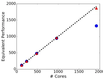
FIGURE 4. Scalability plot. Blue circles: test performed with 200 rays; red triangles: test performed with 1000 rays; dashed line: ideal curve.

case retained for the scalability test is the laboratory scale burner whose computational domain is made of 8 millions cells. Tests have been conducted on a range of cores, from 120 up to 1920. Two tests have been performed with a fixed number of rays emit-ted in each point of the domain (200 for the first case, 1000 for the second one), and no convergence criteria have been imposed. The test characterized by a lower number of emitted rays presents some disadvantageous conditions to scalability, as a huge number of communications between slaves and master is required. The results of the scalability analysis are summarized in Fig. 4 where it can be noticed a perfect ability of the method to require less wall-clock time as the number of processors is increased up to 1000 cores. When the cores number is higher than 1000, the time to exchange the informations between the master process and the slaves improves. Consequently the case with a lower number of rays prevents to achieve good scalability at larger process counts because of an overload of the master, which increases in propor-tion to the number of processes used. On the contrary, when the load of the slaves grows, a linear scalability is accomplished up to 1920 cores, with no deviation from the ideal scalability curve, meaning that the scalability limit is not reached. This trend let us expect that strong scalability will continue further, for a larger number of processors.

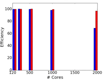
The efficiency plot in fig. 5 confirms the code performance. In the case characterized by the overloading of the master, the ef-ficiency decreases to 70 % for a large number of cores, while, for the second case, it remains close to 100% whatever the number of cores.

FIGURE 5. Efficiency bar chart. Blue: test performed with 200 rays; red: test performed with 1000 rays.

Local Convergence

As already mentioned, one of the main interests of the ERM method is the possibility to control the local convergence. To show this feature, instantaneous snapshots of unsteady 3D DNS simulations of the turbulent channel flow, defined in fig. 1, are used to solve the radiation field.

To estimate the local standard deviation the actual total number of optical paths (N) is divided into n packages with N/n optical paths for each package. In order to evaluate the convergence of a Monte Carlo solution, the control is done on the relative and the absolute value of the standard deviation. The relative standard deviation is the ratio of the local standard deviation to the local radiative power. However, this parameter is not enough as there can be some regions, such as the injector of a combustion chamber, where there are no participating gases, and the radiative power is zero. Therefore the absolute value of the local standard deviation, is checked to be lower than a prescribed maximum.

The ERM method is simulated in two different cases: in the first one a given number of realizations, or optical paths, is imposed to be the same for all the nodes of the domain; in the second one a local convergence criterion is imposed. For all the simulations the gases spectral properties are computed using the correlated κ -distribution [18].

Case 1: Simulations with a fixed rays number In this test, the rays number is imposed to 10,000 for all the com-puted points. To evaluate the achieved level of convergence, it can be interesting to take a look at the standard deviation of the

FIGURE 6. Field of RMS of radiative power on a transversal section of the channel (top). Plot of RMS of radiative power (red) and tempera-ture (blue) on the same section obtained with the Monte Carlo ERM in fixed rays number tests (bottom).

radiative power. This variable, together with the temperature, is plotted over the y-axis of the channel in Fig. 6, showing that a better accuracy is reached in the region near the hot wall of the channel, while high values of rms radiative power are encoun-tered in the colder regions of the channel.

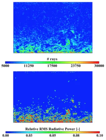
Case 2: Simulations with imposed convergence criteria This test case is set-up in such a way that calculations are performed until the relative criterion is lower than 5% or the locale absolute value of the standard deviation is lower than 10% of the maximum value of the mean radiative power. Here the number of rays generated from each cell is not anymore set a priori, but it varies spatially according to the local standard deviation. The local convergence controlling algorithm makes possible to relate the local standard deviation to the local number of optical paths: the fig. 7 shows that in regions where the convergence is difficult to achieve, more optical paths are provided, or equivalently that the regions characterized by a number of shots lower then the maximum, have achieved the convergence.

To conclude it can be confirmed that the radiative power field predicted by ERM is easier to converge in high temperature re-gions where the accuracy is bigger. The reason of the differ-ent behavior in hot and cold zones lies in the frequency distribu-tion funcdistribu-tion used in ERM, as it is based on the spectral emitted power. Consequently the optical paths issued from colder cells are characterized by low frequencies. But the radiative power ab-sorbed by a cold cell has mainly be emitted by hot regions, emit-ting at much higher frequencies. The absorbed radiative power is

FIGURE 7. Number of rays (top) and relative standard deviation (bot-tom) obtained with the Monte Carlo ERM in controlled convergence.

then strongly underestimated in cold regions. This phenomenon does not appear for hot cells as the emitted radiation spectrum is very close to the absorbed one [11]. These considerations clearly show that the distribution function used in the ERM method may not be optimized for fast convergence in the cold regions, leading to excessive CPU time.

MONTE CARLO OERM

To alleviate the mentioned problem different methods exist, one of the most important ones is the so-called importance sam-pling: a variance reduction method to accelerate Monte Carlo convergence. This is the core of the Optimized Emission-based Reciprocity Method (OERM) [11], where the frequency distri-bution function is chosen in such a way as to correct the ERM drawback and decrease the variance.

In the OERM method the frequency distribution function, fν(ν,Tmax), is based on the emission distribution at the

maxi-mum temperature encountered in the system and it is expressed

as fν(ν,Tmax) = κν(Tmax)Iν○(Tmax) ∫+∞ 0 κν(Tmax)Iν○(Tmax)dν . (5)

In these conditions, the radiative exchange power for unit volume between i and j, given by (2), can be expressed as

P_{i j}exch=P_ie(Tmax)∫ +∞ 0 I○ ν(Ti) I○ ν(Tmax) κν(Ti) κν(TImax) (6) [I ○ ν(Tj) I○ ν(Ti) −1] fν(ν,Tmax)dν fΩidΩi

The use of the pdf (5) allows to eliminate the disadvantage of the classical approaches of ERM in the cold regions. To il-lustrate the advantages of the OERM method, computations of the radiative transfer in the channel flow are performed. In a first step solutions of radiative field obtained with a OERM approach are obtained with the same computation conditions of the case 1, at imposed number of rays, and they are compared to the so-lutions obtained with the ERM method. The standard deviation for both of the methods is exhibited in Fig. 8: on the hot wall results of ERM and OERM overlap as the two frequency distri-bution functions are practically identical, therefore OERM turns into ERM. Focusing on the colder regions on the bottom of the section, the same figure shows that the standard deviation in the OERM case is much lower than in the ERM case, meaning that with the same number of realizations, the frequency distribution function of OERM allows the absorption by the cold regions to be more accurately computed, contrary to the case of ERM. Consequently if a convergence criterion is fixed, calculations conducted with an OERM method need a lower number of re-alizations to satisfy the same criterion as it can be seen in fig. 9, leading to a less expensive computational cost.

The OERM method is now investigated on a semi-industrial configuration, the burner of fig. 3. The temperature, pressure, CO2and H2Omolar fractions used in OERM simulations are

in-stantaneous values extracted from unsteady 3D Large Eddy Sim-ulations of the flow. As seen in Fig. 10 most of the domain emits energy through radiative heat transfer (negative radiative power); the regions where energy absorption dominates (positive radia-tive power) are the coldest gas pockets mainly located in thin layers near the walls.

In the set-up of this case relative and absolute values of stan-dard deviation are controlled in order to insure that the simula-tion completes in a limited CPU time, so a maximum number of rays emitted per point is imposed. If the simulation is locally stopped because of this criterion, the convergence is not achieved in these points. Tests are performed limiting the maximum num-ber of possible optical paths departing from the nodes to 10 000

FIGURE 8. Instantaneous field of rms of radiative power obtained with Monte Carlo OERM (top). Plot of the rms of radiative power for ERM (blue line) and OERM (red line) in test with fixed rays number.

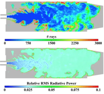
and 20 packages of 500 realizations each are taken into account for the error estimation. The convergence condition of the Monte Carlo algorithm is that of an rms lower than 3 % of the mean value; while in the regions where the criterion of relative rms is never satisfied, a control on the absolute value of the rms, whose value is imposed at 3 % of the maximum value of the mean radia-tive power, is done. In the fig. 11 gray zones are the ones where the absolute criterion is respected, keeping in mind that in these zones the rms of the radiative power is close to zero, while in the remaining part of the chamber a control on the relative error is done. It can be seen that zones where it is most difficult at-tain the established convergence criterion are characterized by a larger number of realizations.

FIGURE 9. Plot of the number of rays needed for the ERM (blue line) and OERM (red line) in controlled convergence.

FIGURE 10. Instantaneous fields of Radiative Power (top) and the opposite of the emitted power (bottom). Black line is the iso-contour for radiative power = 0.

QUASI MONTE CARLO

If the technique used in the OERM method is aimed to reduce the variance through importance sampling; another ap-proach to improve the Monte Carlo error is to replace the pure random sampling with a quasi-random (also called low-discrepancy) sampling, without modifying the frequency distri-bution function. Lower error and improved convergence may be attained by replacing the pseudo-random sequences using low-discrepancy sequences, whose points are distributed in a way to provide greater uniformity (fig. 12). For this study a Sobol se-quence has been used and its construction uses results from [19].

FIGURE 11. Number of rays (top) and relative rms of radiative power (bottom) obtained using the Monte Carlo OERM method.

Using this alternative sampling method in the context of multi-variate integration is usually referred to as Quasi Monte-Carlo, that can be seen like a deterministic version of Monte Carlo method.

Its advantage lies in enhancing the convergence rate [20]. It is possible to asses the error using a Randomized Quasi-Monte Carlo [12]. In the context of radiation simulations, as for the Monte Carlo, n packages are considered; within each of this package, a low discrepancy sequence of N/n points is used, while the n sequences of the packages are randomized using an I-binomial scrambling [21]. This approach allows to benefit from the faster convergence rate of Quasi-Monte Carlo within each package and to have an estimation of the error using the variance between the packages, as it is done for the Monte Carlo method. The obtained Quasi-Monte Carlo method can be combined with both ERM and OERM methods, so that a comparison with the Monte Carlo simulations, previously presented, can be con-ducted. Only OERM results are considered in the following.

Quasi Monte Carlo combined with OERM method

Simulations with a Quasi-Monte Carlo method in its OERM version have been conducted on snapshots of 3D LES of the lab-oratory scale burner. In a first step, simulations have been carried out setting the same number of optical paths departing from all the nodes of the domain, without imposing convergence criteria. Such an analysis allows to evaluate the accuracy of both methods. In fig. 13 the relative standard deviation for both the methods is shown on the whole longitudinal section of the chamber. It can be seen that with the same number of realizations, QMC

simu-FIGURE 12. Sampling of polar (θ ) and azimuthal angle (φ ) using a Sobol sequence (left) and a random sequence (right).

lations are more accurate than MC ones, as the relative error is much lower on the whole domain, even in the zones more diffi-cult to converge, such as the ones close to the cold walls of the chamber.

In order to compare the convergence rate of Monte Carlo and Quasi Monte Carlo simulations, in a second step tests of conver-gence are performed. Their set-up is the same of OERM sim-ulations of the previous chapter, in terms of maximum number of rays and packages, and parameters for the control error. Tests withs local convergence control allow to highlight the advantage of QMC in terms of computational cost. As expected, the number of realizations necessary to respect the convergence criterion is much lower in the case of QMC simulations as showed in fig. 14.

CPU efficiency of Monte Carlo and Quasi-Monte Carlo methods

A more complete comparison can be done evaluating the ef-ficiency of both Monte Carlo and Quasi Monte Carlo methods. The local efficiency of both the methods has been compared and evaluated as

ηi=

1

σ_i2⋅nbint,i⋅(TCPU/nbint,tot)

(7)

where i represents the considered point, nbint,iis the number of

the intersections of the point i, TCPU/nbint,tot is the cost of an

in-tersection. In the fig. 15 the ratio of the local efficiencies of quasi Monte Carlo algorithm and Monte Carlo is showed on a longitu-dinal plane of the chamber: the ratio is bigger than 1 on almost the whole domain, meaning that the QMC method improves the efficiency of the MC, by a value that can be greater than 5, de-pending on the considered points of the domain.

FIGURE 13. Instantaneous field of rms of radiative power obtained with Monte Carlo OERM (top) and Quasi-Monte Carlo OERM (bottom) at imposed number of rays.

FIGURE 14. Number of rays necessary for the convergence used by Monte Carlo OERM (top) and Quasi-Monte Carlo OERM (bottom) in controlled convergence.

In order to localize the regions where Quasi Monte Carlo becomes more efficient, it is interesting to look at the scatter plot of the efficiency ratio in relation to the temperature for all the do-main points and it is shown in Fig. 16. It is worth noting that this ratio is high in the cold pockets of the chamber near the walls, where normally the convergence is hard to be achieved, and that the regions characterized by a higher efficiency ratio are the ones at intermediate temperature (around 1000 K), which cover most of the domain.

Concerning the computational time needed for the simula-tions of the two retained geometries under the best case scenario (Quasi Monte Carlo-OERM in controlled convergence tests), a

FIGURE 15. 2D map of the ratio between efficiency of Quasi-Monte Carlo and Monte Carlo methods.

FIGURE 16. Scatter plot of temperature in relation to the efficiency ratio between Quasi-Monte Carlo and Monte Carlo for all the points of the domain.

radiative solution needs 70 CPU hours for the channel flow con-figuration, while for the semi-industrial burner the amount of CPU hours increases up to 190, running both the computations with 168 cores. The computational cost of coupled simulations can then be estimated a priori. When fluid and radiation solvers are coupled, two parameters should be taken into account: the number of cores dedicated to each code and the coupling fre-quency, i.e. how many iterations fluid and radiation solvers ex-change data:

NfT_CPUf = TCPUr (8)

where T_CPUf and T_CPUr represent the cost of one iteration of the fluid and radiative solver, respectively, and Nf the number of

fluid iterations. If the coupling is performed each time step, the cost of a coupled simulation becomes 10 000 times more expen-sive than a combustion simulation, thus meaning that the radia-tion solver would need a big number of cores to ensure the same

elapsed time than the fluid solver. In order to make the com-putation more affordable, the choice of the coupling frequency parameter becomes significant; for instance, coupling each 2000 fluid iterations, a coupled simulation would become 10 times more expensive than a combustion simulation.

CONCLUSION

Monte Carlo methods applied to radiative heat transfer prob-lems are known for being computationally expensive. In order to afford coupled 3D simulations of reactive flows, it is neces-sary to reduce the computational cost. Different strategies have been proposed to face this limit, some of them, like the ERM or the OERM methods, have been used in this study. Finally a technique to further improve the efficiency of Monte Carlo method, based on a low-discrepancy sampling, has been applied and the obtained quasi-Monte Carlo method has been combined with OERM and compared to the Monte Carlo in a complex con-figuration. Simulations results have shown a significant improve-ment from the quasi-Monte Carlo in terms of computational ef-ficiency, introducing them as an excellent candidate for coupled high-fidelity simulations.

ACKNOWLEDGMENT

This project has received funding from the European Unions Horizon 2020 research and innovation programme under the Marie Sklodowska-Curie grant agreement No 643134. It was also granted access to the HPC resources of CINES under the allocation 2016-020164 made by GENCI.

REFERENCES

[1] Coelho, P. J., 2007. “Numerical simulation of the inter-action between turbulence and radiation in reactive flows”. Progress in Energy and Combustion Science, 33, pp. 311– 383.

[2] Coelho, P. J., 2012. “Turbulence-Radiation Interac-tion: From Theory to Application in Numerical Simula-tions”. Journal of Heat Transfer-Transactions of the ASME, 134(3).

[3] Deshmukh, K. V., Modest, M. F., and Haworth, D. C., 2008. “Direct numerical simulation of turbulence-radiation inter-actions in a statistically one-dimensional nonpremixed sys-tem”. JOURNAL OF QUANTITATIVE SPECTROSCOPY & RADIATIVE TRANSFER, 109(14), SEP, pp. 2391–2400. [4] Deshmukh, K. V., Haworth, D. C., and Modest, M. F., 2007. “Direct numerical simulation of turbulence-radiation interactions in homogeneous nonpremixed combustion sys-tems”. Proceedings of the Combustion Institute, 31(1), pp. 1641–1648.

[5] Zhang, Y., Vicquelin, R., Gicquel, O., and Taine, J., 2013. “Physical study of radiation effects on the boundary layer structure in a turbulent channel flow”. International Jour-nal of Heat and Mass Transfer, 61, pp. 654–666.

[6] Soucasse, L., Riviere, P., and Soufiani, A., 2014. “Subgrid-scale model for radiative transfer in turbulent participat-ing media”. Journal of Computational Physics, 257(A), pp. 442–459.

[7] Gupta, A., Haworth, D., and Modest, M., 2013. “Turbulence-radiation interactions in large-eddy simula-tions of luminous and nonluminous nonpremixed flames”. Proceedings of the Combustion Institute, 34(1), pp. 1281 – 1288.

[8] Walters, D. V., and Buckius, R. O., 1992. “Rigorous de-velopment for radiation heat transfer in nonhomogeneous absorbing, emitting and scattering media”. International Journal of Heat and Mass Transfer, 35(12), pp. 3323 – 3333.

[9] Tess´e, L., Dupoirieux, F., Zamuner, B., and Taine, J., 2002. “Radiative transfer in real gases using reciprocal and for-ward monte carlo methods and a correlated-k approach”. International Journal of Heat and Mass Transfer, 45(13), pp. 2797–2814.

[10] Cherkaoui, M., Dufresne, J.-L., Fournier, R., Grandpeix, J.-Y., and Lahellec, A., 1996. “Monte carlo simulation of radiation in gases with a narrow-band model and a net-exchange formulation”. Journal of Heat Transfer, 118, pp. 401–407.

[11] Zhang, Y., Gicquel, O., and Taine, J., 2012. “Optimized emission-based reciprocity monte carlo method to speed up computation in complex systems”. International Journal of Heat and Mass Transfer, 55(25–26), pp. 8172 – 8177. [12] Lemieux, C., 2009. Monte carlo and quasi-monte carlo

sampling. Springer Science & Business Media.

[13] Kersch, A., Morokoff, W., and Schuster, A., 1994. “Radia-tive heat transfer with quasi-monte carlo methods”. Trans-port Theory and Statistical Physics, 23(7), 09, pp. 1001– 1021.

[14] Guiberti, T. F., Durox, D., Zimmer, L., and Schuller, T., 2015. “Analysis of topology transitions of swirl flames in-teracting with the combustor side wall”. Combustion and Flame, 162(11), pp. 4342–4357.

[15] Guiberti, T., Durox, D., Scouflaire, P., and Schuller, T., 2015. “Impact of heat loss and hydrogen enrichment on the shape of confined swirling flames”. Proceedings of the Combustion Institute, 35(2), pp. 1385–1392.

[16] Mercier, R., Guiberti, T., Chatelier, A., Durox, D., Gicquel, O., Darabiha, N., Schuller, T., and Fiorina, B., 2016. “Ex-perimental and numerical investigation of the influence of thermal boundary conditions on premixed swirling flame stabilization”. Combustion and Flame, 171, pp. 42–58. [17] Koren, C., Vicquelin, R., and Gicquel, O., 2017.

“High-fidelity multiphysics simulation of a confined premixed swirling flame combining large-eddy simulation, wall heat conduction and radiative energy transfer”. ASME Turbo EXPO 2017 (Submitted).

[18] Taine, J., and Soufiani, A., 1999. “Gas radiative properties: From spectroscopic data to approximate models”. Vol. 33 of Advances in Heat Transfer. Elsevier, pp. 295 – 414. [19] Joe, S., and Kuo, F. Y., 2008. “Constructing sobol

se-quences with better two-dimensional projections”. SIAM Journal on Scientific Computing, 30(5), pp. 2635–2654. [20] Hlawka, E., 1961. “Funktionen von beschr¨ankter variatiou

in der theorie der gleichverteilung”. Annali di Matematica Pura ed Applicata, 54(1), pp. 325–333.

[21] Tezuka, S., and Faure, H., 2003. “I-binomial scrambling of digital nets and sequences”. Journal of complexity, 19(6), pp. 744–757.