HAL Id: hal-01159037
https://hal.inria.fr/hal-01159037
Submitted on 2 Jun 2015HAL is a multi-disciplinary open access archive for the deposit and dissemination of sci-entific research documents, whether they are pub-lished or not. The documents may come from teaching and research institutions in France or abroad, or from public or private research centers.
L’archive ouverte pluridisciplinaire HAL, est destinée au dépôt et à la diffusion de documents scientifiques de niveau recherche, publiés ou non, émanant des établissements d’enseignement et de recherche français ou étrangers, des laboratoires publics ou privés.
for Markov random field super-resolution mapping of
remotely sensed images
Hossein Aghighi, John Trinder, Samsung Lim, Yuliya Tarabalka
To cite this version:
Hossein Aghighi, John Trinder, Samsung Lim, Yuliya Tarabalka. Fully spatially adaptive smooth-ing parameter estimation for Markov random field super-resolution mappsmooth-ing of remotely sensed images. International Journal of Remote Sensing, Taylor & Francis, 2015, 36 (11), pp.2851-2879. �10.1080/01431161.2015.1049381�. �hal-01159037�
Fully spatially adaptive smoothing parameter estimation for Markov
random field super-resolution mapping of remotely sensed images
H. Aghighia,c*, J. Trindera, S. Lima, and Y. Tarabalkab
aSurveying and Geospatial Engineering, School of Civil and Environmental Engineering, The
University of New South Wales, Sydney, NSW 2052, Australia; bInria Sophia-Antipolis Méditerranée, TITANE Team, 06902 Sophia Antipolis, France; cDepartment of Remote
Sensing & GIS, Faculty of Earth Science, Shahid Beheshti University, Tehran, Iran (Received 6 December 2014; accepted 19 February 2015)
This article presents a fully spatially adaptive Markov random field (MRF)-based super-resolution mapping (SRM) technique to produce land-cover maps at a finer spatial resolution than the original coarse-resolution image. MRF combines the spectral and spatial energies; hence, an MRF-SRM technique requires a smoothing parameter to manage the contributions of these energies. The main aim of this article is to introduce a new method called fully spatially adaptive MRF-SRM to automatically determine the smoothing parameter, overcoming limitations of the previously proposed approaches. This method estimates the number of endmembers in each image and uses them to assess the proportions of classes within each coarse pixel by a linear spectral unmixing method. Then, the real pixel intensity vectors and the local properties of each coarse pixel are used to compute the local spectral energy change matrix and the local spatial energy change matrix for each coarse pixel. Each pair of matrices represents all possible situations in spatial and spectral energy change for each coarse pixel and can be used to examine the balance between spatial and spectral energies, and hence to estimate a smoothing parameter for each coarse pixel. Thus, the estimated smoothing parameter is fully spatially adaptive with respect to real pixel spectral vectors and their local properties. The performance of this method is evaluated using two synthetic images and an EO1-ALI (The Advanced Land Imager instrument on Earth Observing-1 satellite) multispectral remotely sensed image. Our experiments show that the proposed method outperforms the state-of-the-art techniques.
1. Introduction
Super-resolution mapping (SRM) (Tatem et al. 2002), also called sub-pixel mapping (Verhoeye and De Wulf 2002), is a land-cover classification technique which aims to produce a classified map at a finer spatial resolution than an original coarse-resolution image (Kasetkasem, Arora, and Varshney 2005). The idea of SRM was introduced by Atkinson (1997) to achieve sub-pixel vector boundaries using spatial dependence max-imization. In general, spatial dependence means that the neighbouring pixels may belong to the same class with a high probability (Atkinson 1991).
Generally, SRM methods can be divided into two main categories (Li, Du, and Ling
2012): (1) methods which are applied as post-processing techniques and require soft classification results, and (2) those which can be categorized as classification approaches and are independent of soft classification methods. Most previous works on SRM are related to the first approach, e.g. those based on sub-pixel swapping (Luciani and Chen
*Corresponding author. Email:[email protected]
© 2015 Taylor & Francis
2011; Thornton, Atkinson, and Holland 2006; Xu and Huang 2014), multiple end-member spectral mixture analysis (Powell et al. 2007), geostatistics (Boucher and Kyriakidis 2006; Atkinson, Pardo-Iguzquiza, and Chica-Olmo 2008; Wang, Shi, and Wang 2014), and spatial attraction which was first introduced by Mertens, De Baets, et al. (2004). The key issue of the last method is to find the neighbouring sub-pixels or pixels which should attract the target sub-pixel. Based on this key question, the spatial attraction methods can be categorized as sub-pixel/sub-pixel spatial attraction methods (Wang, Wang, and Liu 2012a; Liguo, Qunming, and Danfeng 2012), pixel, sub-pixel/pixel spatial attraction methods (Mertens et al. 2006; Wang, Wang, and Liu
2012b), spatial attraction between and within pixels (Wang, Wang, and Liu 2012a), hybrid sub-pixel/sub-pixel and sub-pixel/pixel spatial attraction for SRM (Ling et al.
2013), and the multiple shifted image-based attraction model (Xu, Zhong, and Zhang
2012).
Another approach that has received considerable coverage in the literature is based on utilizing heuristic methods to improve the SRM accuracy by maximizing the spatial dependence and generating the spatial distribution of land cover within the mixed pixels, such as using Hopfield neural networks (Tatem et al. 2001), feed-forward backpropaga-tion neural networks (Mertens, Verbeke, et al. 2004), combination of the observation model and backpropagation neural networks (Zhang et al. 2008), genetic algorithms (Mertens et al. 2003), particle swarm optimization (Wang, Wang, and Liu 2012b), and artificial immune system optimization method (Zhong and Zhang 2013).
The second main approach of SRM was first proposed by Kasetkasem, Arora, and Varshney (2005) which employed Markov random field (MRF) because of its suit-ability for representing the spatial dependence between pixels. This method was developed based on three main assumptions: the pixels of the fine spatial resolution image are pure, SRM satisfies the MRF properties, and the pixel intensities for each class in the fine resolution image are normally distributed. In contrast to the first SRM type described earlier, the results of this method do not rely on the availability of accurate class boundaries nor a sub-pixel classified map derived by another method (Kasetkasem, Arora, and Varshney 2005).
One of the theoretical challenges in using MRF is balancing the contributions of spectral and spatial energies, which are controlled by a weight or a smoothing parameter (Aghighi et al. 2014). This internal parameter should be estimated before the MRF-SRM can be applied. It has been demonstrated that a too large weight of the contribution of the spatial energy term yields an over-smoothed classified map (Tolpekin and Stein 2009). On the other hand, if this weight is too small, the available spatial information is not fully utilized; hence, a change in the land-cover fractions is not significant (Li, Du, and Ling 2012). In order to overcome this limitation, Kasetkasem, Arora, and Varshney (2005) estimated four smoothing parameter values for their first-order Markovian energy by employing the Maximum Pseudo-Likelihood Estimation (MPLE) algorithm. Each of the values was estimated for one of the cliques utilizing a high-spatial-resolution ground-reference land-cover map (Kasetkasem, Arora, and Varshney 2005). One major drawback of their approach is that the proposed parameter estimation method requires multiple spatial resolution reference data, which are rarely available in practice. Another problem with this method is that every sub-pixel uses the same weighting coefficient in the same clique direction regardless of whether it is in a heterogeneous or a homogeneous region.
To overcome these limitations, Tolpekin and Stein (2009) proposed another smoothing parameter estimation method based on the analysis of the local energy
balance. They examined the impact of class spectral separability on the balance of spectral and spatial energies with respect to different scale factors between the coarse resolution image and SRM. Finally, they concluded that the smoothing parameter is affected by class separability, scale factor, the neighbourhood system size, configura-tion of class labels, and the choice of the power-law index. A drawback of this method is that a fixed optimal smoothing parameter value is estimated from the average class spectral separability of the entire original image and therefore the local land-cover class properties within each coarse pixel are ignored. Although this method overcomes some of the limitations in the Kasetkasem, Arora, and Varshney (2005) approach, both methods adopted fixed smoothing parameter values which led to an improvement in the classification accuracy in homogeneous areas, but an increased risk of the sub-pixels being over-smoothed in heterogeneous regions such as at class boundaries. This is because class boundaries need lower smoothing parameter values to preserve the edges, and homogeneous regions require higher smoothing parameter values to remove isolated patches (Zhang et al. 2011).
Recently, Li, Du, and Ling (2012) followed the Tolpekin and Stein (2009) method and proposed a spatially adaptive MRF-based sub-pixel mapping (MRF-SPM) model to overcome the limitation of a fixed smoothing parameter. The main concept of their method was that, due to different proportions of land-cover classes within each pixel, the spectral information of remotely sensed images is always spatially variable. Thus, smoothing parameter estimation should be locally adaptive to pixel spectral information. For this reason, they computed the weighted mean of the classes’ spectral separability for all pixels using pixel class proportions estimated by a soft classification method. Although the accuracy assessment has shown that Cohen’s kappa index (κ) value has increased when compared to the method of Tolpekin and Stein (2009), both approaches have several limitations such as using an empirical value instead of local class label configuration to estimate the spatial energy change and assumption of the equal class covariance matrix.
In order to overcome these limitations, a fully spatially adaptive MRF-based SRM method (fully spatially adaptive MRF-SRM) is introduced in this article. This robust framework is developed under the Gaussian class conditional density assumption, and utilizes the local properties of the spatial and spectral information to manage the contribu-tions of spatial and spectral energy terms in the MRF-SRM model. For this reason, a linear spectral unmixing (LSU) method is employed to estimate the fraction of class information within each coarse pixel. Then, this information is utilized to generate an initial super-resolution map (SR-map) for each coarse pixel. The spectral information of each coarse pixel and the configuration of its corresponding sub-pixel class labels from the initial SR-map are used to estimate the spectral energy change. Furthermore, another factor is estimated which represents the spatial energy change using the class label configurations by introducing a class label co-occurrence matrix of the coarse (CLCMC) pixels.
By employing SRM methods, it is possible to generate a detailed information on the shape and geometry of the objects at a finer spatial resolution; thus, the precision of an SRM method should be evaluated based on the quality of the characterization of the shape of objects on the ground. However, most of the previous SRM investigations simply used Cohen’s kappa statistics (κ) (Tolpekin and Stein 2009; Li, Du, and Ling 2012; Mertens et al. 2006) and overall accuracy (OA) (Kasetkasem, Arora, and Varshney 2005), which means that they ignored the geometrical properties of objects. In order to overcome this limitation, this study adopted the Persello and Bruzzone (2010) method which was proposed for accuracy assessment in classification of very high resolution images, and employed the method for the accuracy assessment of MRF-SRM results.
The outline of this article is as follows: Section 2 introduces the details of the MRF-SRM model, and explicitly explains the framework of the previous smoothing parameter estimation methods and the proposed fully spatially adaptive MRF-SRM, including (1) estimation of spectral energy changes, (2) computation of class label configuration, and (3) optimization by simulated annealing. The data description and experimental results are presented and discussed in Section 3. Finally, conclusions are drawn in Section 4.
2. Materials and methods
An input image is denoted by Y ¼ fyi2 RB; i¼ 1; 2; . . . ; mg, where B is the number of
spectral channels and m ¼ N1" N2 is the number of pixels in the image. The spatial
resolution of image Y is denoted as R; therefore, each pixel yi represents a square area of
size R2 on the ground. It is assumed that the spectral intensity of each pixel y
idepends on
the corresponding unobserved pixel label in L ¼ ,! j; j¼ 1; 2; . . . ; m" (Bouman and
Shapiro1994), where each ,j takes its value from a finite set of M thematic classes of
interest Ω ¼ fω1; ω2; . . . ; ωMg. Although image Y was captured by an airborne or a
spaceborne sensor, it was assumed that this image was generated by degradation of a not directly observed image (X) with the same spectral bands and a spatial resolution r. Every pixel of X is assumed to be pure and thus can be assigned to a unique class (Tolpekin and Stein2009). Another assumption is that the spectral intensities of pixels in X, which belong to the same class, as well as the spectral intensities of pixels in Y, are spatially uncorrelated. The ratio between the coarse pixel spatial resolution (R) and the fine pixel spatial resolution (r) is called the scale factor (S ¼ R=r) and is assumed to be an integer value. Hence, each coarse pixel of Y consists of S2 pixels of X and the corresponding positions
of fine pixels within yi can be indexed by xcji, where c ¼ 1; 2; . . . ; S2. By excluding the
partial overlaps between the coarse and fine pixels, the relationship between each coarse pixel of Y and its corresponding finer pixels of X can be established as follows (Li, Du, and Ling 2012): yi ¼ 1 S2 XS2 c¼1 xcji: (1) 2.1. Super-resolution mapping
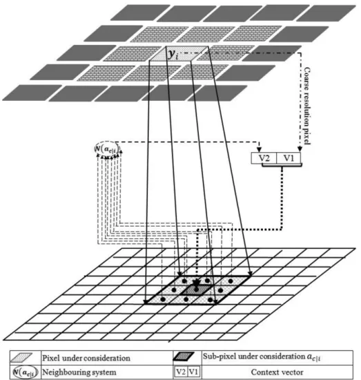
The aim of SRM is to produce a classified map CSRM at a finer spatial resolution (r), and
at the same spatial resolution as X, from a coarse-resolution image (Y) (Figure 1) (Atkinson 2009).
In order to produce the classified SR-map, CSRM, given the coarse spatial resolution
image Y, the Bayes rule is employed in this study:
p Cð SRMjYÞ / p YjCð SRMÞp Cð SRMÞ; (2)
where p Cð SRMjYÞ is the posterior probability of the classified SR-map, CSRM, given the
observed image Y, p YjCð SRMÞ is the class-conditional probability for image Y given the
SR-map (CSRM), and pðCSRMÞ is the prior probability distribution for the SR-map CSRM.
The optimal classified SR-map C%
SRM given the image Y can be generated by solving the
maximization problem for the a posteriori probability (MAP) decision rule (Equation (2)).
C% SRM ¼ argmax CSRM p Cð SRMjYÞ f g ¼ argmax CSRM p YjCð SRMÞp Cð SRMÞ f g: (3)
According to the complexity of Equation (3), which involves the optimization of a global distribution of the image, and due to the equivalence of MRF and Gibbs random field, this optimization can be resolved by minimizing the sum of local posterior energies (Tolpekin and Stein (2009)):
U Cð SRMjYÞ ¼ 1 & λð Þ U YjCð SRMÞ þ λU Cð SRMÞ; (4)
where U Cð SRMjYÞ is the posterior energy function of the classified SR-map CSRM given
the observed image Y, U YjCð SRMÞ is the spectral energy function (likelihood energy) of
the observed image Y given true SR-map CSRM, and UðCSRMÞ is the spatial energy
function (prior energy function). In this equation, λ is called the smoothing parameter (λ ¼ q= 1 þ qð Þ, 0 ( λ < 1), which manages the contribution of spectral and spatial energies, where 0 ( q < 1 controls the overall magnitude of weights. Employing a too large value of λ results in over-smoothing, while a too small value does not lead to sufficient change in the land-cover fractions of a coarse pixel.
Figure 1. MRF-based SRM using spectral and spatial information. (Adapted from Fan and Xiang-Gen (2001).)
Under the assumption of independent and identically distributed (IID) spectral values, the likelihood of yi given CSRM#acji$ can be written as (Kasetkasem, Arora,
and Varshney 2005) PðYjCSRMÞ ¼
Y
i;c
PðyijCSRMðacjiÞÞ;
¼Y i;c 1 ð2πÞB=2j j!i 1=2" exp & 1 2 ðyi& μiÞ TX&1 i ðyi& μiÞ % & ; (5)
where CSRM#acji$is the assigned class to cth sub-pixel of ith coarse pixel. Moreover, the
likelihood energy is then expressed as USpectralðYjCSRMÞ ¼ X i;c U y# ijCSRM#acji$$¼ X i;c 1 2ðyi&μiÞ T !&1i ðyi&μiÞþ 1 2ln !j ji ' ( ; (6) where yi in Equations (5) and (6) is the spectrum vector of the coarse pixel i, which is assumed to be normally distributed with mean μi and covariance !i. Both μi and !i
depend on the pixel composition and can be computed using μi¼X M α¼1 θαiμα; (7) !i ¼ XM α¼1 θαi!α; (8)
where θP αiis the proportion of the class ωα in the composition of coarse pixel yi, such that M
α¼1 θαi ¼ 1, and μα and !α are the mean and covariance of the class ωα, respectively,
which are estimated using a sufficient number of pure training pixels (Kasetkasem, Arora, and Varshney 2005).
The spatial energy term in Equation (4), U Cð SRMÞ, is modelled as (Li, Du, and Ling
2014) U Cð SRMÞ ¼ X c;i U C# SRM#acji$$; ¼X c;i X al2N að Þcji ϕ að Þ " 1 & δ Cl # # SRM#acji$; CSRMð Þal $$; (9)
where U C# SRM#acji$$is the local spatial energy of the sub-pixel CSRM#acji$and N a# cji$is
the neighbourhood system for sub-pixel acji(Figure 1). In this equation, CSRM#acji$is the
class label of the central sub-pixel and CSRMð Þ is the class label of its surroundingal
neighbours. The spatial dependence is computed by using the Kronecker delta function ðδ ,# i; ,j$¼ 1 if ,i ¼ ,jand δ ,# i; ,j$¼ 0 if ,i!,jÞ; φ að Þ depends on d al # cji; al$, which is
a geometric (Euclidean) distance between the central sub-pixel acji and its spatial neigh-bour al (Equation (10)) (see Figure 2) (Makido and Shortridge 2007):
φ að Þ ¼l 1η
d a# cji; al$
r
% &&g
; (10)
where η is the normalization constant so that Pl2N a cji
ð Þ η að Þ ¼ 1, r is the pixel size ofl
SR-map, and the power-law index g is usually set as g ¼ 1 (Li, Du, and Ling 2012). 2.2. Spatial and spectral energy balance analysis
As discussed, the accurate labelling of the sub-pixels relies on the smoothing parameter, which manages the contributions of the spatial and spectral energies. Based on this theory, Tolpekin and Stein (2009) proposed a method to estimate this parameter by analysing the balance between spatial and spectral energies. They assumed that a class label of a given sub-pixel CSRM#acji$¼ α is assigned to an incorrect class label CSRM#acji$¼ β within a
coarse pixel. Therefore, based on Equation (3), one can infer:
U C# SRM#acji$¼ αjyi$) U C# SRM#acji$¼ βjyi$: (11)
By substituting the corresponding terms in Equation (11) and solving this inequality equation, a limited number of λ values can be estimated from the balance between the change in the prior ("Uαβspat) and the likelihood energy ("Uαβspec) values:
"Uαβspat ( "Uαβspec: (12)
"Uαβspat can be estimated as
"Uαβspat¼ q X l2N að Þcji ϕ að Þl ' δ β; Cð SRMð Þal Þ & δ α; Cð SRMð Þal Þ ( ) ) ) ) ) ) ) ) ) ) ) ) ) ) ) ) ) ) ¼ qγ; (13)
where γ is a parameter related to the prior energy coefficient φ, the neighbouring window size, and to the configuration of pixel class label CSRMð Þ in the N aal # cji$ of a specific
image. Furthermore, the spectral energy change "Uαβspec before and after updating the pair
Figure 2. Neighbourhood system and geometric distance between the sub-pixels d a# cji; al$.
of sub-pixel labels was formulated by using the Mahalanobis distance between two classes:
"Uαβspec ¼12*μβS& μ2 α+T!&1i μβ& μα S2
* +
; (14)
where due to the equal covariance matrix assumption !i ¼ 1=Sð 2Þ !α.
By computing "Uαβspecand "Uαβspat; a range of values for the smoothing parameter that satisfies Equation (12) can be found; therefore, by solving "Uαβspec ¼ "Uαβspat and recalling λ ¼ q= 1 þ qð Þ, the optimal smoothing parameter for a pair of classes can be found as
λ%¼ 1
1 þ"Uγspec
: (15)
Here, "Uspecis proposed as the mean of "Uspec
αβ in the case of the difference between
class separability for different pairs of classes: "Uspec ¼ PM&1 α¼1 PMβ¼αþ1"Uαβspec M M&1ð Þ 2 : (16)
It was demonstrated that λ > λ%will result in over-smoothing and a very small value of
λ does not fully utilize the spatial information.
2.3. Spatially adaptive MRF-SPM
Although the method of Tolpekin and Stein (2009) proposed an efficient way for estimating a smoothing parameter, it suffered from the limitation of using a fixed λ%
value for the entire image. Estimating λ% by Tolpekin and Stein (2009) is a non-adaptive
MRF-SRM method, because it does not take into account the fact that the spectral information of the remotely sensed pixels is spatially variable due to different types and proportions of land-cover classes within each coarse pixel. Therefore, Li, Du, and Ling (2012) utilized an adaptive smoothing parameter in terms of the local spectral energy for a given coarse pixel "Uispec, which is computed using the pixel class proportions derived from the spectral unmixing method:
"Uispec ¼ PM&1
α¼1
PM
β¼αþ1θαiθβi"U spec αβ
PM&1
α¼1 PMβ¼αþ1θαiθβi
; (17)
where θαi and θβi represent the class proportions for classes α and β in pixel yi,
respectively, and PM&1α¼1 PMβ¼αþ1θαiθβi is the normalizing weight. In the case of a pure
coarse pixel belonging to the class α, "Uispec can be written as
"Uispec ¼ PM
β¼1;β ! α" Uαβspec
M & 1 : (18)
The advantage of using "Uispecin Equations (17) and (18) in comparison with "Uspec
in Equation (16) is that "Uispec employs the local properties provided by the pixel spectra
in calculating the smoothing parameter. Thus, the higher proportion classes gain more weight in "Uispec. The adaptive smoothing parameter is then estimated as follows:
λ% i ¼
1 1 þ"Uγispec
: (19)
2.4. Fully spatially adaptive MRF-SRM
The spectral statistics of classes show that the mean and covariance of the classes are different (Richards and Jia 2006). However, Tolpekin and Stein (2009) and Li, Du, and Ling (2012) assumed the same covariance matrices for all classes; hence, they employed the Mahalanobis distance (Equation (14)) to estimate the change in the spectral energy "Uαβspec in a coarse pixel of the original image. Another limitation of both methods is that they did not use the real spectral information vector of each coarse pixel to compute the spectral energy change. This means that they ignored the complexity of the real world by computing the Mahalanobis distance between two classes with the same covariance matrix for the whole image. This assumption does not satisfy the IID requirement that is claimed to exist in both methods.
In another simplification, Tolpekin and Stein (2009) proposed Equation (16) to simply compute the average of spectral energy change ("Uspec) for the entire image
based on spectral energy change of each pair of classes "Uαβspec. In order to overcome this limitation, Li, Du, and Ling (2012) proposed a weighted mean which employed the class proportion of each coarse pixel to compute "Uispec (Equation (17)). Their basic concept is that, when a coarse pixel does not contain a land-cover class ωj, there
is no chance that their model misclassifies CSRM#acji$ as class ωj. Although this
assumption is correct, they inappropriately simplified the model. That is because the class label of a sub-pixel located on the borders of a given coarse pixel (CSRM#acji$in
Figure 3) can be changed or swapped by the class label of another sub-pixel (CSRMð Þal
in Figure 3) on the border of a neighbouring coarse pixel. For instance, the class label of CSRM#acji$ in Figure 3 can be replaced with the probability of 5=9 by a class label
of a neighbouring coarse pixel, because this sub-pixel is located in a corner of pixel yi
and the second-order neighbourhood system is employed. This probability will be increased by utilizing a higher-order MRF neighbouring system. Thus, it can be concluded that the neighbouring coarse pixels have a direct impact on the spectral energy change "Uαβspec of a given coarse pixel yi.
Tolpekin and Stein (2009) introduced a constant empirical value for the entire image (γ) instead of estimating the spatial energy change ("Uαβspat) which was also employed by Li, Du, and Ling (2012) into Equations (15) and (19). This parameter γ depends on the weighting function of the spatial energy, MRF neighbourhood system size, and the configuration of class labels (Tolpekin and Stein 2009). This means that γ should vary significantly for each coarse pixel based on the configuration of class labels. Moreover, the proportions of land-cover classes within each coarse pixel (employed in Equation (17)) and the class label configuration of the coarse pixels will change during the optimization process. Hence, it is important to use the class labels of neighbouring sub-pixels of each given coarse pixel for estimating the spatial energy change.
This article therefore presents a new framework for a fully spatially adaptive MRF-SRM method under the Gaussian class conditional density assumption. This method has been developed based on concepts similar to those of Tolpekin and Stein (2009) and Li,
Du, and Ling (2012); however, the local properties of both spatial and spectral informa-tion are utilized to analyse the spatial and spectral energies.
In this method, the initial class proportions of each coarse pixel are extracted from the fractional information of the classes generated using an LSU method (Hu, Lee, and Scarpace 1999). In this research, the LSU method is employed because it assumes that the endmembers are distributed side-by-side within the sensor field of view (Plaza et al.
2007), which is the same as the final output of SRM. The selected LSU is a constrained LSU model, where the sum of its abundance results is one.
In this research, the Geometry-based Estimation of the Number of Endmembers-Affine Hull (GENE-AH) algorithm (Ambikapathi et al.2013) is employed to systematically estimate the number of endmembers in our data sets (the implemented software: mx.nthu.edu.tw/~ tsunghan/download/GENE_codes.zip). Then, the fast pixel purity index method was imple-mented via the Research Systems ENVI 4.5 (Environment for Visualizing Images) software package to extract the endmembers and apply the LSU method.
In the next step, the scale factor S and the estimated initial class proportion of each coarse pixel using LSU were utilized to generate the initial SR-map, by sub-dividing each coarse-resolution pixel yi into S2 sub-pixels. Then, based on the fractional abundance of
Figure 3. Changing the sub-pixel class label CSRM#acji$ based on a sub-pixel class label in
neighbouring coarse pixel CSRMð Þ. Sub-pixel Cal SRM#acji$has got nine sub-pixel neighbours five
of which are located in the neighbouring course pixels.
each classes (fj) within a given coarse pixel yi, a specific number of sub-pixels Fjtakes the
value ,j from the data set Ω ¼ ωf 1; ω2; . . . ; ωMg:
Fj ¼ roundðfj* S2Þ; (20)
where round +ð Þ returns the value of the closest integer. Although Villa et al. (2011) proposed (Equation (20)) to calculate the number of sub-pixels which should be assigned to class ,j in yi, usually the value of Pj¼ωj¼ωM1 Fj! S
2. Hence, in each coarse pixel, some
classes are randomly selected using the roulette wheel selection method (Burke, Newall, and Weare 1996). In order to create the roulette wheel for each given coarse pixel yi, each individual section of the roulette wheel is proportional to fj of that pixel. Then, the wheel
is spun a number of times equal to the value of S2
&Pj¼ωM j¼ω1 Fj ) ) ) ) )
) to select some individual class labels of the coarse pixel. Then, based on the sign and value of S2
&Pj¼ωM
j¼ω1 Fj
* +
, this process adds/removes the number S2&Pj¼ωM
j¼ω1 Fj ) ) ) ) )
) of sub-pixels to/from Fj of the
selected classes. The newly computed Fj is called FjEdit and the results of this procedure
prove that the value of Pj¼ωM
j¼ω1 F
Edit
j ¼ S2. Then, the FjEdit number of sub-pixels in a given
coarse pixel yi is randomly selected and is assigned to classes ,j to produce the initial
SR-map CInit
SRM#acji$.
2.4.1. Spectral energy change
In order to develop the fully spatially adaptive MRF-SRM framework, the spectral and spatial energy changes for each coarse pixel should be estimated. Consider that the class label of a sub-pixel within a given coarse pixel yi changes from a true label CSRM#acji$¼
α to a false label CSRM#acji$¼ β. This misclassification leads to the changes in the
composition of the coarse pixel, and consequently changes in the mean and covariance matrix of each coarse pixel from the current solution (μCur; !Cur) to a new solution
(μNew; !New) by Equations (7) and (8). Also, the local likelihood energy value
(Equation (6)) of a given coarse pixel changes from the energy of current solution (UCur
spec) to a new energy value in the revised solution (UspecNew). These values can be used
to compute the spectral energy change ("Uspecαβ ) for a given pixel:
"Uαβspec¼ UspecNew& UspecCur
) ) ) ) ) ): (21)
The class label of each sub-pixel can change from one element of Ω ¼ ωf 1; ω2; . . . ; ωMg
to another member of the Ω data set. Therefore, "Uαβspec for each coarse pixel can be computed for M2 different situations to generate a global square matrix (M " M) of
"Uαβspec with zero diagonal elements for each coarse pixel (see Table 1):
Each element of this table shows the spectral energy change in a given coarse pixel by changing a sub-pixel class label from α (a class in rows) to β (a class in columns) as a new solution. In order to fill out this table for each coarse pixel, one value from the frequency of the first selected class should be decreased and one value to the frequency of the second selected class should be increased. Then, the configuration of these new solutions should be utilized to compute (μNew; !New) using Equations (7) and (8) as well as (UspecNew) by
employing Equation (6).
In order to compute the class label configuration of each coarse pixel, a window is employed which contains its corresponding sub-pixel and the sub-pixel rows and columns on the border of its neighbouring coarse pixels (Figure 3). The number of utilized neighbour-ing rows and columns are defined by the order of MRF neighbourneighbour-ing system; for example, in the case of second-order neighbouring system, a nearest row and column of sub-pixels which are located on the border of its neighbouring coarse pixels are sufficient, because each pixel within a given coarse pixel will be updated using the class label of one of those sub-pixels. Hence, the window size for second-order MRF neighbouring system could be simply formulated as S þ 2ð Þ " S þ 2ð Þ. Then, the frequency of each class label for a given coarse pixel is computed using the sub-pixels within its corresponding window.
It should be noted that during the optimization process, if a new solution for a given coarse pixel is accepted, then the global matrix of "Uαβspec of that coarse pixel should be updated. Furthermore, if the frequency of a specific class in a given coarse pixel is zero, then the spectral energy change related to that class does not contribute to the smoothing parameter estimation of that coarse pixel ( 0
"Uαβspec ¼ 0, see Equation (19)).
2.4.2. Spatial energy change
The value of γ in Equation (13), which describes the spatial energy change "Uαβspat, is related to φ, which can be computed using Equation (10), the neighbouring window size (2S & 1) and the configuration of pixel class labels of a specific image. However, due to updating the class labels configuration for each accepted solution, the smaller window size
S þ 2
ð Þ " S þ 2ð Þ is proposed in Section 2.4.1.
In order to define "Uαβspat for each coarse pixel, a CLCMC pixel (Ψ), which is a square matrix with the same size as the global matrix of "Uαβspec, is defined (Table 2). This matrix provides information about the spatial frequency distribution of each pair of classes in the window (Aghighi et al. 2014).
Since S2is the number of sub-pixels within a given coarse pixel y
i, and this study uses
the second-order neighbouring system, each central sub-pixel acji is surrounded by N a# cji$¼ 8 sub-pixels (al). The Ψ index is computed for each coarse pixel yi using the
sub-pixels within its corresponding window:
Table 1. Global matrix of "Uαβspec for given coarse pixels.
Class 1 Class 2 . . . Class M Class 1 "U1;1spec¼ 0 "U1;2spec "U1;...spec "U1;Mspec Class 2 "U2;1spec "U2;2spec¼ 0 "U2;...spec "U2;Mspec
: : : : :
Class M "UM;1spec "UM;2spec "UM;...spec "UM;Mspec ¼ 0
Table 2. Global matrix ofΨωα;ωβ for a given coarse pixel.
Ψ1;1 Ψ1;2 Ψ1;... Ψ1;M
Ψ2;1 Ψ2;2 Ψ2;... Ψ2;M
: : : :
ΨM;1 ΨM;2 ΨM;... ΨM;M
Ψωα;ωβ ¼ XS2 c¼1 X N að Þcji l¼1 ϕ að Þδ Cl # SRM#acji$; ωα$δ C# SRMð Þ; ωal β$; (22)
where,Ψωα;ωβ is theΨ for class ωα with class ωβ. In this equation, CSRM acji # $
is the class label of the central sub-pixel of the coarse pixel yi and CSRMð Þ is the class label of itsal
surrounding course pixel al within the window of yi. The computed global matrix of
Ψωα;ωβ shows the frequency of neighbouring classes for each coarse pixel. Thus, it should be normalized based on the number of sub-pixels within a window ðS þ 2Þ2 and N a# cji$in γωα;ωβ ¼ Ψωα;ωβ S þ 2 ð Þ2" N a# cji$ : (23) In the next step, the smoothing parameter for a given pixel yi can be estimated using
λαβð Þi ¼ 1 1 þ γð Þi "Uspec αβ iðÞ ; (24)
where γð Þi ¼ γωα;ωβ computed by Equation (23) for a given coarse pixel i and "U
spec αβð Þi is the spectral energy change for pixel i. Thus, λαβð Þi is a square matrix (M " M). The adaptive smoothing parameter for a given coarse pixel λ%
i is computed using the weighted average by
employing pixel class proportion: λ% i ¼ PM&1 α¼1 PMβ¼αþ1θαiθβiλαβð Þi PM&1 α¼1 PMβ¼αþ1θαiθβi : (25)
The parameters of this function are explained in Equation (17). Notably, the pixel class proportion should be updated in each iteration.
2.5. Optimization and estimation
In this work, a simulated annealing (SA) algorithm as a heuristic optimization technique is employed to iteratively search for a solution to the proposed fully spatially adaptive MRF-SRM model. A change is proposed at each iteration and it is accepted if it decreases the objective function. On the other hand, if it increases the objective function, it is accepted with a certain probability exp &δ=kð BTÞ, where δ is the energy of the system, T is the
temperature, and kB is a physical constant called Boltzmann constant (Eglese1990). The
annealing schedule is based on the following power-law decay function:
Titer ¼ σTiter&1; (26)
where Titer is the temperature at the iteration ‘iter’, and σ 2 0; 1ð Þ controls the rate of the
temperature decrease.
After generating the initial SR-map and setting the starting iteration number (iterstart ¼ 1), the maximum number of iterations (itermax), starting temperature T0, cooling
down constant σ, and termination condition, the SA producer will be continued until the
termination conditions are satisfied. In this work, two termination conditions are used: iter ) itermax or the number of sub-pixels successfully updated during three consecutive
iterations is less than 0.1% (Tolpekin and Stein 2009).
2.6. Validation
As mentioned earlier, most of the previous SRM investigations ignored the evaluation of the geometrical properties of the objects on the ground generated by SRM methods and simply utilized κ and OA (Tolpekin and Stein2009; Li, Du, and Ling2012; Mertens et al.
2006; Kasetkasem, Arora, and Varshney 2005). In addition to κ, OA, and average accuracy (AA), four error measures (e) proposed by Persello and Bruzzone (2010) are adopted in this work: (1) over-segmentation error (eOSE
i ), which refers to the subdivision
of a single object into several distinct regions Equation (27); (2) under-segmentation error (eUSE
i ), which refers to fusing different objects into a single region (Equation (28)); (3)
edge location error (eELE
i ), which measures the precision of the generated object edges
with respect to the reference map (Equation (29)); and (4) fragmentation error (eFGE i ),
which refers to sub-partitioning of single objects into different small regions (Equation (30)). eOSEi ðOi; RiÞ ¼ 1 &jOiO\ Rij i j j ; (27) eUSE i ðOi; RiÞ ¼ 1 &jOi\ Rij Ri j j ; (28) eELEi ðOi; RiÞ ¼ 1 &je Oð Þ \ e Rie O ð Þi j i ð Þ j j ; (29) eFGEi ðOi; RiÞ ¼ ri& 1 Oi j j & 1: (30)
Here each error can be computed for a given pair Oð i; RiÞ, where O ¼ Of 1; O2; . . . ; Odg is
a set of d objects in the reference map and R ¼ Rf 1; R2; . . . ; Rrg indicates a set of r
regions with four- or eight-connectivity pixels in the classified map. Each pixel in the region Rj is assigned to class ,j fromΩ ¼ ωf 1; ω2; . . . ; ωMg, and +j j in Equations (27)–
(30) represents the cardinality of a set. In these equations, Ri is the corresponding region
in the thematic map with the highest number of common pixels with a given object Oi in
the reference map. Moreover, Oj i\ Rij is the overlapping area among the region Ri and
the object Oi. Also, eð+Þ is an operator which extracts the borderline of objects with a
width greater than 1 pixel, and ri in Equation (30) is the number of regions that have at
least one overlapping pixel with the region Oi. The fragmentation error is scaled in the
0; 1
½ -, and the other error values are scaled to 0;½ 1Þ. Smaller error values which are close to 0 mean better results for eOSE
i , eELEi , and eFGEi and worse accuracies for eUSEi
In order to compute eELE
i , three different situations are considered, for which the
results were denoted as B1, B2, and B3, respectively. In the case of ELE-B1, the reference map with one pixel wide edges has been used. However, for other cases of ELE-B2 and ELE-B3, the edge widths in the reference map are doubled or considered as buffer pixel widths around the edges, respectively.
Persello and Bruzzone (2010) estimated the global error eð Þh from the local errors eð Þh ¼ 1 d Xd i¼1 eð Þih : (31)
In Equation (31), the size of regions is ignored, while by employing Oj j in Equation (31),i
the weighted global error measurement can be computed. Since the estimated weighted global error measurement by the Persello and Bruzzone (2010) equation was not in the range of 0; 1ð Þ, it can be formulated as
eð Þh ¼ 1 Pd i¼1j jOi Xd i¼1 Oi j jeð Þih: (32)
Because of the lack of space, the details of the algorithm are omitted, and for more information, refer to Persello and Bruzzone (2010).
Finally, McNemar’s tests (χ2) were applied to evaluate the statistical significance of
the difference in accuracy between each pair of classified maps with the 5% significance level (Foody 2004).
3. Experimental results and discussion 3.1. Synthetic images
Before using our fully spatially adaptive MRF-SRM technique to generate SR-map of real data sets, the simulated data have been used to compare the accuracy of the fully spatially adaptive MRF-SRM generated map to those obtained by using other MRF-based SRM techniques. For this reason, the methodology of Yu and Ekström (2003) and Mohn, Hjort, and Storvik (1987) is adopted to generate the simulated images, where it is assumed that the distribution of pixel intensities is based on a multivariate Gaussian distribution. Moreover, the pixel intensity for a given pixel i is independent of the corresponding class label and also independent of the autocorrelated noise process. In order to identify the distribution parameters, Mohn, Hjort, and Storvik (1987) denoted μc for the mean vector and defined the covariance matrix to be 1 & θð ÞρcΓ, where θ and ρc are
propor-tional factors and Γ is a fixed B " B positive definite matrix.
According to Yu and Ekström (2003), each image is considered to have two bands (B ¼ 2)
and three classes, where covariance matrices, ρcs, for each class are 0.4, 1.4, and 1.0, respec-tively. Therefore, the distribution of the classes with larger ρ is less peaked than the distribution of the classes with lower values. In this article, the largest ρ value belongs to class 2; hence, most of these pixels which belong to this class and fall into the intersection between the classes will be misclassified (Yu and Ekström2003; Mohn, Hjort, and Storvik1987).
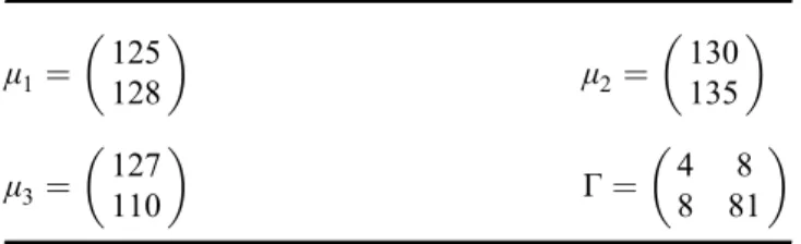
Table 3gives the values for the mean of each class and matrix Γ, adopted from Mohn, Hjort, and Storvik (1987) and used in our experiments. Parameter θ was set to 0.5.
By utilizing the mentioned parameters, the covariance matrix for each class is computed (Table 4).
Mohn, Hjort, and Storvik (1987) reported the 16.5% error rate for the classification of the simulated image using the maximum likelihood classification technique (specifically 37% error rate for class 2 and around 10% error rate for classes 1 and 3).
In order to generate a synthetic image with regularly shaped objects, a multispectral (MS) Système Pour l’Observation de la Terre (SPOT) image at 2.5 m resolution compris-ing 300 by 300 pixels (Figure 4(a)) is utilized.
The image was captured from the Mildura region in the state of New South Wales, Australia. Then, it was manually digitized into three different classes with non-simple regularly shaped objects and considered to be a fine spatial resolution reference map for regularly shaped objects (Figure 5(a)).
Another synthetic image comprising 300 by 300 pixels with irregularly shaped objects (Figure 4(f)) was generated by adopting the irregularly shaped object reference map of Li, Du, and Ling (2012) and using a subset of an image in Shanghai, China, from Google Earth (31.1203800N; 121.3605600E) (Figure 4(e)). However, the class borders of the
refer-ence map were changed and the map was converted into three classes (Figure 6(a)). In the next step, by utilizing the mean and covariance of the classes (Table 4), two fine-resolution images (regularly shaped object (Figure 4(b)) and irregularly shaped objects (Figure 4(f)) with two bands and three classes were generated by sampling from the multivariate normal distribution (Li, Du, and Ling 2012). Then, the produced image for regularly shaped objects (Figure 4(b)) was degraded with S ¼ 10 and the image with
irregularly shaped objects (Figure 4(f)) was degraded with S ¼ 6 to produce the degraded
coarse-resolution images (Figures 4(c) and (g)).
3.2. The real remote-sensing image
In order to evaluate the performance of the developed method using real remote-sensing imagery, a data set which was provided by the United States Geological Survey through the online facility known as EarthExplorer (http://earthexplorer.usgs.gov) is utilized. This image was acquired by the ALI sensor installed on the first Earth-Observing (EO-1) spacecraft. This spaceborne sensor simultaneously captured panchromatic (PAN) (Figure 4(i)) and MS data (Figure 4(j)) with nine spectral bands with spatial resolution
Table 3. The proposed values for the mean of each class and matrixΓ. μ1 ¼ 125 128 % & μ2¼ 130 135 % & μ3 ¼ 127110 % & Γ ¼ 48 818 % &
Source: Adapted from Mohn, Hjort, and Storvik (1987).
Table 4. The mean and covariance for each class based on the Yu and Ekström (2003) method. !1¼ 0:81:6 16:21:6 % & !2¼ 2:85:6 56:75:6 % & !3¼ 24 40:54 % & μ1 ¼ 125 128 % & μ2 ¼ 130 135 % & μ3 ¼ 127 110 % &
of 10 and 30 m at nadir, respectively. Thus, the scale factor between MS and PAN images is S ¼ 3.
The selected study area is a subset of the image over the farmland in five points, CA 93624, USA, which in the Universal Transverse Mercator (UTM) projection is located between upper-left X coordinates: 224,756.3, upper-left Y coordinates: 4,027,896.3 and
Figure 4. (a) SPOT multispectral (MS) image; (b) synthetic image of regularly shaped objects with a scale factor of 1; (c) degraded synthetic image of regularly shaped objects with a scale factor of 10 (the image is zoomed by a factor of 10); (d) degraded synthetic image of regularly shaped objects (Figure 4(c)) zoomed by a factor of 1; (e) Google Earth image; (f) synthetic image of irregularly shaped objects with a scale factor of 1; (g) degraded synthetic image of irregularly shaped objects with a scale factor of 6 (the image is zoomed by a factor of 6); (h) degraded synthetic image of regularly shaped objects (Figure 4(g)) zoomed by a factor of 1; (i) the panchromatic image of EO1-ALI (The Advanced Land Imager instrument on Earth Observing-1 satellite) sensor; (j) the MS image of the EO1-ALI sensor (RGB: 743); (k) the real proportional size of the MS image of the EO1-ALI sensor (see Figure 4(j)).
lower-right X coordinates: 227,129.8, lower-right Y coordinates: 4,024,648.4 as on 31 July 2012. This image comprises 327 by 240 PAN pixels and their corresponding MS pixels. The reference map (Figure 7(a)) was produced using visual interpretation of the PAN image and the pan-sharpening product. The number of classes is assumed to be 5, which is equal to the estimated number of endmembers using GENE-AH.
3.3. Evaluation of the fully spatial adaptive MRF-SRM method
In order to estimate the efficiency of the proposed fully spatial adaptive MRF-SRM method, this research applies two state-of-the-art SRM methods, namely MRF-based SRM developed by Tolpekin and Stein (2009) (non-adaptive MRF-SRM) and the spatially adaptive MRF-SPM introduced by Li, Du, and Ling (2012) (spatially adaptive MRF-SPM) on both real and simulated data sets. In the case of non-adaptive MRF-SRM, instead of using a fixed smoothing parameter value, different values of the smoothing parameter are utilized. The values vary from a low value of 0.1 to 0.5 (resulting in insufficient smoothing of the image) with an interval of 0.1 and from 0.5 to 0.99 (resulting in the over-smoothing of the image) with an interval of 0.05 to demonstrate the quality of the results in the non-adaptive MRF-SRM. Each algorithm
Figure 5. The regularly shaped objects with straight boundaries. (a) The reference map (300 " 300 pixels) employed to produce original 4 (a); (b) the generated SR-map using degraded image with a scale factor of 10 (see (c) or (d)) from the fully spatial adaptive MRF-SRM method; (c) the generated SR-map using degraded image with a scale factor of 10 (see Figures 4(c) or (d)) from the spatial adaptive MRF-SPM method; (d) the generated SR-map using degraded image with a scale factor of 10 (see Figures 4(c) or (d)) from the non-adaptive MRF-SRM method with the highest overall accuracy and κ; (e) the hard classification results of the original simulated image using an original image with a scale factor of 1 (seeFigure 4(b)) from the SVM method; (f) the hard classification map using degraded image with a scale factor of 10 (seeFigures 4(c) or (d)) from the MLC method.
was run 10 times to obtain reliable results and the OA results of each algorithm are illustrated in Figure 8.
In addition to the mentioned methods, two other state-of-the-art hard classification techniques are utilized, namely the maximum likelihood classifier (MLC) and the support vector machine (SVM) to classify the EO1-ALI MS image (Figure 4(j)), and the degraded simulated images (Figures 4(c) and (g)). In the case of SVM, the LIBSVM library is employed to apply the multiclass one-versus-one SVM classification method using a Gaussian radial basis function kernel (Chang and Lin 2011). The optimal SVM para-meters C and γ were chosen by fivefold cross validation. In each experiment, the similar training data sets were utilized to train both SVM and MLC classification techniques. Finally, the generated maps were extended to S ¼ 1 and the performances of the methods were evaluated by comparison with their corresponding reference maps with S ¼ 1. Thus, the produced edges from both hard classification techniques results are S times wider than the edge width sizes of the reference map as well as generated SR-maps. This unwanted source of errors significantly decreases the values of all computed eELE
i , because it
increases the probability that a given edge pixel in a reference map be covered by a coarse edge pixel in derived maps. Hence, the computed edge error location for both hard classification techniques in Table 7 cannot be trusted.
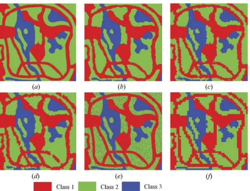
Figure 6. The irregularly shaped objects. (a) The reference map (300 " 300 pixels) employed to produce original 4 (f)); (b) the generated SR-map using degraded image with a scale factor of 10 (see Figures 4(g) or (h)) from the fully spatial adaptive MRF-SRM method; (c) the generated SR-map using degraded image with a scale factor of 10 (see Figures 4(g) or (h)) from the spatial adaptive MRF-SPM method; (d) the generated SR-map using degraded image with a scale factor of 10 (see Figures 4(g) or (h)) from the non-adaptive MRF-SRM method with the highest overall accuracy and κ; (e) the hard classification results of the original simulated image using original images with a scale factor of 1 (seeFigure 4(f)) from the SVM method; (f) the hard classification map using degraded image with a scale factor of 10 (seeFigures 4(g) or (h)) from the MLC method.
The reference and classified maps of simulated data with regularly shaped features (Figures 4(b)–(d)) and irregularly shaped features (Figures 4(g) and (h)), as well as the EO1-ALI data set (Figure 4(j)) are represented in Figures 5–7, respectively.
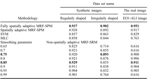
In order to compare the performance of each method on each data set, the estimated OA of the generated SR-map for the regularly shaped objects, irregularly shaped objects, and EO1-ALI remotely sensed images are presented in Figures 8(a)–(c), respectively. According to the highest OA value for each data set in Figure 8, the best smoothing parameter for the regularly shaped objects and EO1-ALI remotely sensed image is 0.85 (Figures 8(a) and (c)) and for the irregularly shaped objects is 0.75 (Figure 8(b)). Moreover, this figure illustrates that the OAs of the proposed fully spatially adaptive MRF-SRM for all data sets are higher than those derived by the other methods as evidenced by κ (seeTable 5) (Cohen 1960).
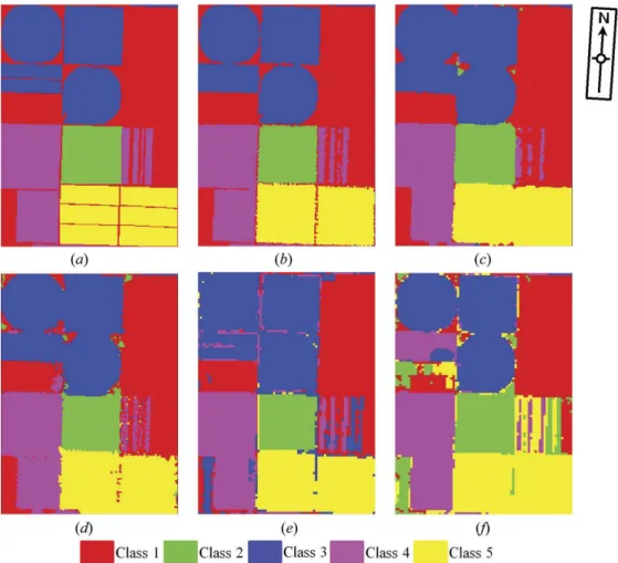
Figure 7. The generated results for the multispectral image of the EO1-ALI sensor. (a) The reference map produced from Figures 4(i)); (b) the generated SR-map using degraded image with a scale factor of 3 (seeFigures 4(g) or (h)) from the fully spatial adaptive MRF-SRM method; (c) the generated SR-map using degraded image with a scale factor of 3 (seeFigures 4(g) or (h)) from the spatial adaptive MRF-SPM method; (d) the generated SR-map using degraded image with a scale factor of 3 (see Figures 4(g) or (h)) from the non-adaptive MRF-SRM method with the highest overall accuracy and κ; (e) the hard classification results of the original simulated image using original image with a scale factor of 1 (see Figure 4(f)) from the SVM method; (f) the hard classification map using degraded image with a scale factor of 3 (see Figures 4(g) or (h)) from the MLC method.
In addition to OA and κ, the produced thematic maps using each method were compared with the reference map to evaluate the accuracy of each individual class for each data set (Table 6). With regard to the sensitivity of the non-adaptive MRF-SRM method, the generated maps with λ ¼ 0:85 for both simulated regularly shaped object image and EO1-ALI remotely sensed image, and with λ ¼ 0:75 for the simulated irregu-larly shaped object image are selected, because they gained the highest OA value (Figure 8(b)) and κ (Table 6). In the following, all these measures of accuracies for each data set will be analysed.
3.3.1. Regularly shaped object image results
As Table 6shows, the highest accuracies for all classes of the simulated regularly shaped object image belong to the fully spatially adaptive MRF-SRM method proposed. However, the OA achieved using different SRM methods are equal or vary by less than 2.1%, while κ varies by 0.08. Thus, McNemar’s test with the 5% significance level was employed to check the null hypothesis (H0) of no significant difference between each pair
of maps accuracy values. The H0 hypothesis was rejected by the computed χ2 for all pairs
of generated maps.
Figure 8. Overall accuracy assessment of the generated SR-map using fully spatial adaptive MRF-SRM, spatially adaptive MRF-SPM, and for non-adaptive MRF-SRM with different smoothing parameters for the (a) regularly shaped objects, (b) irregularly shaped objects, and (c) the EO1-ALI image.
Table 5. The mean κ for the fully spatially adaptive MRF-SRM, spatial adaptive MRF-SPM, support vector machine (SVM), maximum likelihood classification (MLC), and non-adaptive MRF-SRM with different smoothing parameters of both regularly/irregularly shaped object synthetic images and EO1-ALI image.
Data set name
Synthetic images The real image Methodology Regularly shaped Irregularly shaped EO1-ALI image Fully spatially adaptive MRF-SPM 0.937 0.902 0.951 Spatially adaptive MRF-SPM 0.928 0.892 0.917
SVM 0.857 0.863 0.829
MLC 0.858 0.844 0.763
Smoothing parameter Non-spatially adaptive MRF-SRM
0.65 0.825 0.714 0.616 0.7 0.921 0.855 0.616 0.75 0.920 0.893 0.900 0.8 0.921 0.876 0.906 0.85 0.929 0.855 0.911 0.9 0.911 0.838 0.904 0.95 0.904 0.832 0.905 0.99 0.901 0.764 0.616
Table 6. The overall accuracy values for the fully spatially adaptive MRF-SRM, spatial adaptive MRF-SPM, support vector machine (SVM), maximum likelihood classification (MLC), and non-adaptive MRF-SRM with different smoothing parameters of both regularly/irregularly shaped object synthetic images and EO1-ALI image.
Fully spatially adaptive
MRF-SRM Spatially adaptiveMRF-SPM Non-spatially adaptiveMRF-SRM SVM MLC Simulated image – regularly shaped objects
OA 95.8 94.2 93.7 90.3 90.8 AA 95.8 94.3 93.7 90.5 90.9 κ 0.937 0.928 0.929 0.857 0.858 Class 1 95.1 93.2 93.0 94.5 93.5 Class 2 96.2 94.5 93.9 81.8 90.4 Class 3 96.2 94.9 94.0 95.5 88.9 Simulated image – irregularly shaped objects
OA 93.9 93.2 92.1 91.5 90.1 AA 93.9 93.3 92.2 91.5 89.6 κ 0.902 0.892 0.873 0.863 0.844 Class 1 92.1 92.1 90.1 89.4 85.5 Class 2 95.3 94.2 93.7 93.2 96.6 Class 3 94.4 93.5 92.9 91.8 86.8 EO1-ALI remotely sensed data
OA 96.3 93.7 93.2 86.9 81.2 AA 96.9 93.8 93.1 89.4 79.6 κ 0.951 0.917 0.911 0.829 0.763 Class 1 94 93.5 91.6 94.3 99.1 Class 2 99 92.5 92.8 99.8 58 Class 3 97.5 93.4 96.7 76.2 97.8 Class 4 98.3 96.5 91.0 86.5 76.7 Class 5 95.4 92.7 93.4 90.4 66.4
By visual inspection and comparison between the edges in the reference map (Figure 5(a)) and other generated maps, it can be seen that the generated edges using the fully spatially adaptive MRF-SRM technique (Figure 5(b)) presents better details of boundary information than other methods. For instance, both MLC map (Figure 5(f)) and SVM results produced a map with jagged boundaries and results of the spatially adaptive MRF-SPM (Figure 5(c)) and the non-adaptive MRF-SRM (Figure 5(d)) reveal that the detailed boundary information is smoothed or lost.
These qualitatively results are assessed quantitatively using eELE
i (seeSection 2.6) and
the corresponding errors are reported inTable 7. According to this table, the smallest edge location errors for all ELE-B1, ELE-B2, and ELE-B3 are obtained when using the fully spatially adaptive MRF-SRM technique. The differences between ELE-B1 and ELE-B2 values for this method show that by doubling the width of the reference edges, the edge location error decreases by 0.253. By increasing the edge width in the ELE-B3 case, the edge location error value decreases by 0.436 to 0.267. This means that less than 27% of the generated edge pixels using the fully spatially adaptive MRF-SRM method are outside
Table 7. The overall accuracy values for the fully spatially adaptive MRF-SRM, spatial adaptive MRF-SPM, support vector machine (SVM), maximum likelihood classification (MLC), and non-adaptive MRF-SRM with different smoothing parameters for synthetic images with both regularly/ irregularly shaped object and the EO1-ALI image.
MLC SVM Non-spatially adaptiveMRF-SRM Spatially adaptiveMRF-SPM Fully spatially adaptiveMRF-SRM Simulated image – regularly shaped objects
GOS 0.097 0.113 0.077 0.058 0.052 GWOS 0.088 0.095 0.063 0.052 0.042 GUS 0.165 0.217 0.164 0.581 0.596 GWUS 0.088 0.095 0.063 0.631 0.632 GFE 0.001 0.001 0.001 0.002 0.001 ELE-B1 0.843 0.843 0.793 0.739 0.703 ELE-B2 0.696 0.698 0.608 0.538 0.450 ELE-B3 0.552 0.547 0.437 0.363 0.267 Simulated image – irregularly shaped objects
GOS 0.161 0.119 0.111 0.098 0.096 GWOS 0.098 0.085 0.079 0.067 0.06 GUS 0.039 0.025 0.060 0.021 0.016 GWUS 0.008 0.013 0.012 0.012 0.009 GFE 0.002 0.002 0.003 0.003 0.002 ELE-B1 0.751 0.735 0.688 0.663 0.618 ELE-B2 0.543 0.504 0.451 0.415 0.390 ELE-B3 0.364 0.302 0.258 0.224 0.221 EO1-ALI remotely sensed image
GOS 0.187 0.165 0.150 0.169 0.091 GWOS 0.155 0.128 0.072 0.068 0.049 GUS 0.073 0.008 0.315 0.225 0.273 GWUS 0.325 0.151 0.022 0.025 0.015 GFE 0.004 0.006 0.006 0.005 0.007 ELE-B1 0.805 0.774 0.782 0.811 0.616 ELE-B2 0.633 0.594 0.638 0.636 0.431 ELE-B3 0.462 0.444 0.515 0.528 0.295
Note: In this table, GOS, GWOS, GUS, GWUS, GFE, ELE-B1, ELE-B2, and ELE-B3 indicate global over-segmentation, global weighted over-segmentation, global segmentation, global weighted under-segmentation, global fragmentation error, global edge location error without buffer, global edge location error with 2-pixel width reference map, and global edge location error with 3-pixel width reference map, respectively.
of ELE-B1 buffer. However, the corresponding proportions derived using the spatially adaptive MRF-SPM and non-adaptive MRF-SRM methods are 36.33% and 43.68%, respectively. Thus, the performance of the fully spatially adaptive MRF-SRM technique is superior to produce the SR-map for this data set.
The null hypotheses (H0) of no significant difference between each pair of map
accuracy values are rejected for all generated maps due to McNemar’s test with the 5% significance level.
3.3.2. Irregularly shaped object image results
The user accuracies of all methods for each individual class of this data set are presented in Table 6. From the non-adaptive MRF-SRM results, the map generated with a smooth-ing parameter of 0.75 was chosen. In contrast to classes 1 and 3, the highest accuracy for class 2 was achieved by MLC which is 1.3% higher than the fully spatially adaptive MRF-SRM result. This can be explained by comparing the user (96.6%) and producer accuracies (83.3%) of this class which have been computed but not displayed. The producer’s accuracy estimates that 83.3% of class 2 pixels are classified as class 2, while from the user’s accuracy 96.6% of the pixels assigned to class 2 really belong to this class. This means that the mixed pixels on the class edges are not classified as class 2, which leads to lower producer’s accuracy.
A visual comparison of maps generated for this data set (Figure 6) shows that the poorest quality boundaries are generated by the MLC algorithm due to the image spatial resolution (S ¼ 6) (Figure 6(f)). Although the spatially adaptive MRF-SPM map bound-aries (Figure 6(c)) appear to be more accurate than non-adaptive MRF-SRM (Figure 6(d)), both are still more irregular than those derived from the fully spatially adaptive MRF-SRM map (Figure 6(b)). These conclusions from visual inspections are supported by the edge location error values in Table 7, where the estimated ELE for the fully spatially adaptive MRF-SRM is lower than those derived using other methods. For instance, by considering a one pixel buffer around the edges, the edge location error for the fully spatially adaptive SRM is improved by 0.397 and that for spatially adaptive MRF-SPM and non-adaptive MRF-SRM is improved by 0.439 and 0.431, respectively. Although the ELE-B3 obtained using the fully spatially adaptive MRF-SRM method for this data set is lower than a similar result for the simulated image with regularly shaped objects, it should be considered that this error difference could be related to difference in scale factors between both simulated images.
Other geometric error indices reported in Table 7 illustrate that the fully spatially adaptive MRF-SRM errors are mostly less than for other methods; thus, one can infer that the performance of the proposed fully spatially adaptive MRF-SRM technique is superior for producing the SR-map for this data set.
3.3.3. The EO1-ALI image results
The accuracy results of all methods for the EO1-ALI image are presented inTable 6. From the non-adaptive MRF-SRM results, the map generated with a smoothing parameter of 0.85 was chosen. As Table 6 illustrates, the highest accuracies for classes 4 and 5 were achieved for the fully spatially adaptive MRF-SRM and for classes 2 and 3 with a small difference, by SVM and MLC, respectively. However, the highest reported accuracy for class 1 with 5.1% difference from fully spatially adaptive MRF-SRM belongs to MLC. The MLC producer’s accuracy for classes 1 and 2 shows that only 62.6% of class 1 pixels
are classified as class 1. Thus, 37.4 % of the pixels are probably misclassified as other classes such as class 2, which can be seen in the left side of Figure 7(f). Because of this, the user’s accuracy of class 2 was reported to be 58% and its producer’s accuracy was 97.7%. In contrast to SVM and MLC with very large variations of individual class accuracies, the difference between the maximum and minimum accuracies of the other methods used are less than 6.8%.
A visual comparison between the generated maps for this data set (Figure 6) shows that none of these methods can completely extract or regenerate the edges or the class borders. For instance, both SVM and MLC methods missed the roads between the farms or misclassified them as other classes. Although the spatially adaptive MRF-SPM polygon borders appear better than hard classification results as well as the non-adaptive MRF-SRM results, the narrow roads between classes 2 and 5 have been missed. In comparison with other methods, it seems that the narrow roads are regenerated better using the fully spatially adaptive MRF-SRM method.
Based on the edge location error values reported in Table 7, the fully spatially adaptive MRF-SRM regenerated the edges better than the other methods. For instance, the difference between the ELS of fully spatially adaptive MRF-SRM and the lowest ELS value for other methods are 0.158, 0.163, and 0.149 for ELS-B1, ELS-B2, and ELS-B3, respectively. Furthermore, ELE-B3 shows that less than 29% of the generated edge pixels using the fully spatially adaptive MRF-SRM method are not located inside of ELS-B1 buffer around the edges. However, the corresponding proportions for spatially adaptive MRF-SPM and non-adaptive MRF-SRM are 52.8% and 51.5%, respectively. In addition to edge location error indices, other errors reported in
Table 7 illustrate that the lowest GOS, GWOS, and GWUS are achieved using the
fully spatially adaptive MRF-SRM method. Thus, the best agreement between the number of classified regions in the reference map and generated SR-map belongs to the fully spatially adaptive MRF-SRM method. The highest GUS error value belongs to non-adaptive MRF-SRM.
For this data set, McNemar’s test with the 5% significance level rejected the null hypotheses (H0) of no significant difference between each pair of all generated maps.
These data sets were utilized to evaluate the capability of this method to overcome the limitations of other state-of-the-art methods. For instance, the object shapes, the mean and covariance of the classes in the synthetic images, and consequently their Gaussian distributions and also the separability between classes are different. Moreover, the selected real satellite image was chosen from a non-homogenous region which contains diverse land-use/land-cover classes with different class separability. In order to evaluate the ability of the method to preserve the shapes, this study area contains very complex shapes, such as a semi-circle region, triangles, arcs, and very narrow roads between polygons, with the same as well as different classes. Although this research tried to employ some data sets which represent many classification situations occurring in large areas, the performance of the proposed method and other MRF-based SRM methods should be evaluated for very large areas in future research. Because a large area with diverse land-use/land-cover classes would be more complex, it should have some positive impact on approximating the precise means and covariance matrices of classes as well as simultaneously some negative effects on the class separability and the estimation of the fractional abundances of each class in each coarse pixel.
The literature review and the implementation of the algorithms therein raise a chal-lenge to reduce the SRM execution time. Although this research employed some innova-tive methods based on the positional look-up tables to decrease the execution time, it is a
question of future research to propose efficient optimization algorithms to speed up the satisfaction of the termination conditions.
4. Conclusion
The MRF-based SRM technique is a category of SRM methods, which employs the MRF theory and aims to produce land-cover maps at a finer spatial resolution than the original coarse-resolution image. The MRF-based methods require an internal para-meter, called the smoothing parapara-meter, to balance the contributions of spatial versus spectral energies. A too large smoothing parameter value increases the contributions of the spatial energy term and generates an over-smoothed classified map in the bound-aries, while a too small smoothing parameter value does not fully utilize the available spatial information in the homogeneous areas. Thus, it should be estimated before the MRF-SRM can be applied.
The previous smoothing parameter estimation methods used some properties of the entire image to estimate a fixed smoothing parameter value, or ignored the complexity of the image and utilized some simplified or fixed values for image properties to estimate the spatially adaptive smoothing parameter values. In order to overcome these limitations, this study employed the real intensity vectors of each coarse pixel as well as the local properties of each coarse pixel to compute the spectral energy change matrix and the spatial energy change matrix for each coarse pixel. These matrices cover all possible situations in spatial and spectral energy change for each coarse pixel; thus, they can be used to assist the analysis of the balance between spectral and spectral energies. Then, these matrices of each coarse pixel were utilized to estimate the smoothing parameter for each coarse pixel.
In this article, two synthetic images with the regular and irregular shaped objects as well as an EO1-ALI MS remotely sensed image were processed to evaluate the perfor-mance of the fully spatially adaptive MRF-SRM method. The visual inspection of the classified maps showed that the region boundaries and linear features are regenerated more accurately by the fully spatially adaptive MRF-SRM method than by other methods. These results were confirmed using quantitative analysis. It is therefore concluded that the fully spatially adaptive MRF-SRM succeeds in producing land-cover maps at a finer spatial resolution, outperforming the state-of-the-art methods.
Acknowledgements
The authors would to thank the United States Geological Survey which provided EO1-ALI images through the online facility known as EarthExplorer, Murray-Darling Basin Authority which pro-vided the SPOT and very high resolution aerial images, and anonymous reviewers for comments which helped to improve and clarify this manuscript.
Disclosure statement
No potential conflict of interest was reported by the authors.
References
Aghighi, H., J. Trinder, Y. Tarabalka, and S. Lim. 2014. “Dynamic Block-Based Parameter Estimation for Mrf Classification of High-Resolution Images.” IEEE Geoscience and Remote Sensing Letters 11 (10): 1687–1691. doi:10.1109/LGRS.2014.2305913.