HAL Id: hal-02607450
https://hal.inrae.fr/hal-02607450
Submitted on 16 May 2020
HAL is a multi-disciplinary open access
archive for the deposit and dissemination of sci-entific research documents, whether they are pub-lished or not. The documents may come from teaching and research institutions in France or abroad, or from public or private research centers.
L’archive ouverte pluridisciplinaire HAL, est destinée au dépôt et à la diffusion de documents scientifiques de niveau recherche, publiés ou non, émanant des établissements d’enseignement et de recherche français ou étrangers, des laboratoires publics ou privés.
J.C. Mailhol, Rami Albasha, Bruno Cheviron, J.M. Lopez, Pierre Ruelle, C.
Dejean
To cite this version:
J.C. Mailhol, Rami Albasha, Bruno Cheviron, J.M. Lopez, Pierre Ruelle, et al.. The PILOTE-N model for improving water and nitrogen management practices: Application in a
Mediter-ranean context. Agricultural Water Management, Elsevier Masson, 2018, 204, pp.162-179.
The PILOTE-N model for improving water and nitrogen management practices. Application in a Mediterranean context.
J.-C. Mailhol1,*, R. Albasha2, B. Cheviron1, J.-M. Lopez3, P. Ruelle1, C. Dejean1
1 UMR G-Eau, Irstea, Univ. Montpellier, 361 rue Jean-François Breton, BP 5095, 34160 Montpellier Cedex 05, France
2 INRA, UMR 0759 LEPSE, 2 place Pierre Viala, 34060 Montpellier, France
3 CIRAD, UMR G-EAU, 361 rue Jean-François Breton, BP 5095, 34160 Montpellier Cedex 05, France
* Corresponding author
e-mail: jean-claude.mailhol@irstea.fr phone number: +33 (0)4 67 04 63 46 fax number: +33 (0)4 67 16 64 40
Abstract
In this paper we present PILOTE-N, a crop model devoted to the calculation of crop production from the joint water and nitrogen soil status effects. It is the extension of PILOTE, for contexts in which water might not be the sole limiting factor for crop yield, but the same model structure and credo of parsimonious parameterisation have been kept, assuming simplified descriptions of the physical processes at play. One original aspect of PILOTE-N is the calculation of Leaf Area Index (LAI) and cumulative nitrogen plant demand from similar logistic-type functions. LAI is controlled by specific temperature sums, shape parameters and the occurrence of water and nitrogen stresses, while the time average of LAI values over critical phenological periods also affects the predicted harvest index and crop yield. As specific plant parameters are known from PILOTE, calibration was devoted to nitrogen parameters. Which governing the daily-averaged mineralization rate in a first step, then the two shape parameters of the potential nitrogen plant demand (from the dilution curve) in a second step and, at last, which allowing the link between nitrogen uptake and nitrogen of the soil. Model performance was evaluated using multiple initial soil conditions, irrigation and fertilization strategies for corn, durum wheat and sorghum, over a climatic series of 14 years, at the experimental plot of Lavalette (Montpellier, South-East of France), hence in a Mediterranean context characterized by severe, water stresses during summer, typically exceeding nitrogen stresses. Crop yield as well as the dynamics of nitrogen budget were correctly simulated (R2>0.94 for grain yield, total dry matter and nitrogen in plant). The robustness of such a simple and easy-to-calibrate tool is expected to facilitate its use and implementation in other agro-pedoclimatic contexts, to decipher the effect of abiotic stresses and improve irrigation and fertilization scenarios when included in dedicated tools.
Summary
Glossary ... 4
1. Introduction ... 6
2. Material and methods ... 8
2.1. The existing PILOTE model ... 8
2.1.1. Climatic forcings ... 8
2.1.2. Soil module ... 8
2.1.3. Plant module ... 9
2.2. The new PILOTE model: PILOTE-N ... 11
2.2.1. Terms of the nitrogen budget ... 11
2.2.2. Volatilization... 11
2.2.3. Denitrification ... 12
2.2.4. Mineralization ... 12
2.2.5. Nitrogen demand by the plant ... 13
2.2.6. Lixiviation ... Erreur ! Signet non défini. 2.2.7. Nitrogen uptake by the plant ... Erreur ! Signet non défini. 2.2.8. Impact of nitrogen stresses on the harvest index ... 15
2.3. Field experiments and validation data ... 15
3.. Model calibration ... 17
3.1.. Mineralization ... Erreur ! Signet non défini. 3.2... Potential and actual plant Nitrogen uptake ... 18
4. Validation 4.1 LAI and Soil Water reserve (SWR) 4.2 Lixiviation ... 20
4.3. Model evaluation along 14 years ... 22
5. Discussion ... Erreur ! Signet non défini. 6. Conclusion ... 27
Glossary
aN Parameter for the nitrogen stress impact on HI - aw Parameter for the water stress impact on HI
C1 and C2 fixed and progressive N soil compartments
CM Calibration parameter for the potential mineralization kg ha-1 d-1
Cp Partitioning coefficient -
Es Soil evaporation mm
Eta Actual evapotranspiration mm
ETM Maximal evapotranspiration mm
ETo Reference evapotranspiration mm
GY Grain Yield Mg ha-1
HI Harvest index -
HIpot Potential harvest index -
Ka Parameter controlling nitrogen plant uptake -
Kc Crop coefficient -
Kc max Maximal value of Kc -
Kr Ratio between easily usable soil water reserve and TAW -
Ksoil Resistance of soil to evaporation -
LAI Leaf area index m2 m-2
LAIav Average LAI values between Ts1 and Ts2 m2 m-2
LAImax Maximal leaf area index m2 m-2
LAIst Threshold LAIav value m2 m-2
NA Applied nitrogen kg ha-1
ND Nitrogen lost by denitrification kg ha-1
NF Final nitrogen amount kg ha-1
NI Initial nitrogen amount kg ha-1
NL Nitrogen lost by lixiviation kg ha-1
NM Nitrogen amount obtained by mineralization kg ha-1
NP Nitrogen amount in the plant kg ha-1
Nsoil N soil storage kg ha-1
NV Nitrogen lost by volatilization kg ha-1
OM Volumetric organic matter %
PCND Potential Cumulative N plant demand kg ha-1 PCNDmax Maximal cumulative N plant demand kg ha-1
pH Soil pH -
Pr Root depth m
Ps Depth of the first reservoir m
R1, R2, R3 Superficial, root zone and deep soil reservoirs -
Rs Solar radiation J cm-2
Rmax Maximal root depth m
RUE Radiation use efficiency -
T Daily average air temperature °C
TAW Total available water in soil mm m-1
Tb Base temperature °C
TD Threshold temperature for denitrification °C
TDM Total Dry Matter Mg ha-1
Te Temperature for crop emergence °C
TPm Maximal transpiration mm Tm Temperature (in base Tb) to reach LAImax °C Tmin, Tms Temperature thresholds for mineralization °C TMr Reference temperature for mineralization °C
Tp Transpiration mm
Ts1 Temperature of the 1st critical stage °C Ts2 Temperature of the 2nd critical stage °C VM pot Potential permanent mineralization rate kg ha-1 d-1
Vr Root growth rate m d-1
x1, x2 Shape parameters of the nitrogen plant demand curve -
α, β Shape parameters of the LAI curve -
ε Extinction coefficient -
λ Harmfulness of the water and nitrogen stresses -
fc Soil water content at field capacity cm3 cm-3 wp Soil water content at permanent wilting point cm3 cm-3 R2 Normalized water content of the R2 reservoir -
1. Introduction
Irrigation is necessary for ensuring crop growth under a wide range of climatic conditions going from Tropical Wet to Arid regions (FAO, 2013), allowing 40% of world crops over 20% of cropped lands (FAO, 2015). Water availability for irrigation is however increasingly constrained by prolonged rainfall deficits induced by climate change and the increasing competition among agriculture, industry, tourism and urban areas, urging the agricultural sector to improve water productivity (Molden and Oweis, 2007. More precisely, the optimization of water and nitrogen use efficiencies is most often deemed to achieve sustainable crop production while preserving the environment. This requires a change of paradigm in the numerous cases in which fertilisation practices were largely established under non-limiting water and nitrogen availability conditions: the merits and drawbacks of these irrigation and fertilisation strategies should plausibly be re-evaluated from wider perspectives. For example, Nitrogen (N) is necessary to crop growth and to obtain a good yield but excessive N applications with respect to plant N requirements can have substantial negative impacts on the surface waters, the water table and the farmer's income.
The optimal management of the water-nitrogen couple is a serious challenge today in agricultural contexts concerned by strong input reductions (Agostini et al., 2010). By contrast, Quemada et al. (2013) have recently conducted a review on existing strategies to reduce nitrate leaching from cropped lands. The authors highlighted that tailoring irrigation supply to crop requirements is the most efficient method for reducing nitrate leaching with reductions reaching as much as 78% of nitrate leaching from fields with poorly-managed irrigation calendars. Modelling appears as an appropriate tool to tackle this resources management optimization problem and a non-negligible number of efficient crop models have been developed for this purpose, but the use of most of these models is constrained by data availability. This pleads for the development of crop models requiring a limited number of parameters that may be calibrated from an affordable observation effort.
Some models are crop-specific such as CERES-Wheat (Richie et al., 1984), CERES-Maize (Jones et al., 1986) or ARCWHEAT (Weir et al., 1984). This crop specificity allows sometimes the introduction of several adaptive mechanisms, drawn from genetics, to mitigate water stresses (Casals 1996). Other models are more generic such as EPIC (Williams et al., 1989), DAISY (Hansen et al., 1990) and STICS (Brisson et al., 1998, 2003). Although such models are renowned scientific tools, their lack of flexibility (Affholder and al. 2012) and especially their typically high parameterisation costs limit their application for operational field management purposes. This again
legitimates the development of lighter crop models, characterized by a limited number of sensitive parameters, while acknowledging limited objectives compared to these of the full physical basis approaches. Then the minimal expectations for models designed from the principle of parsimony could be to describe first-order physicochemical processes "well enough" to provide the correct temporal dynamics for the main observable quantities involved in the water and N budgets (e.g. soil water reserve, N amount in soil solution, mineralization rate, nitrogen uptake by plant roots).
Regarding N fate, most of the cited models calculate the plant N demand according to the critical N concentration required for the accumulation of biomass to start while STICS or DAISY rely on an optimum N concentration curve. Whatever the degree of sophistication of the N mineralization module, the process needs knowledge of soil organic matter and it is governed by soil temperature and humidity. Most models use a capacitive approach for the soil water balance, in which solute or nutrient leaching is based on the convection-dispersion equation involving mixing between two successive reservoirs, as for example in STICS that appeals to the Burns (1974) solute transfer approach. In PILOTE-N as in STICS, soil-related processes are simulated using a capacitive approach while plant-related processes are process-based. However, PILOTE-N has more limited objectives regarding yield components (and some aspects of nitrogen management) compared to STICS, resorting to a limited number of parameters.
In the world of crop models, the PILOTE model (Mailhol et al., 1997; Khaledian et al., 2009; Mailhol et al., 2011) is one irrigation management tool that has been built for operational field management objectives. It is the agronomic and the hydrological core of the Optirrig software (Cheviron et al., 2016) turned towards the generation, analysis and optimization of irrigation scenarios, and the coupling between both tools was made easier and more efficient by the relatively simple nature of PILOTE.
The objective of this paper is to describe the development of a new nitrogen management component of PILOTE. The latter has been widely used in different regions of France and Maghreb assuming that water was the sole limiting factor for crop yield. Satisfactory results were generally obtained. However, under peculiar conditions, some gaps between measured and simulated yields have suggested to add a nitrogen component to PILOTE in order to reach a more comprehensive description of abiotic stresses. More into details, the opportunity to connect or disconnect the nitrogen module, thus to use PILOTE or PILOTE-N, is a convenient method for understanding the origin of possible gaps and to decipher the relative magnitude of the abiotic stresses. This study therefore exposes the choice of new model components in coherence with the structure and the simplicity level of the pre-existing PILOTE model. To our knowledge, no similar research was
conducted in a Mediterranean context where the plant can suffer from high water stress during summer, and where the dynamics of N uptake appear rather specific (Nemeth, 2001; Poch Massegù, 2012). The strength of the followed approach is also reinforced by the diversity of the experimental conditions over the 14 years of the climatic series. Some treatments are fully irrigated, little irrigated or conducted under rain-fed conditions. Regarding nitrogen, the initial N soil storage is sometimes high or low associated with different N applications, in addition combined with different climatic conditions. By contrast, it is not unusual that similar research relies on two years only, one for calibration, the other for validation. This is the case for instance of the study conducted by Salo and al., 2016) devoted to the comparison of 11 crop models which highlights the great variability of the model results. This may encourage the development of one’s own model.
2. Materials and methods
2.1.
In the following sections, we will first briefly describe the structure of
the existing PILOTE model. The description of the new nitrogen-based
processes follows then.
The existing PILOTE model2.1.1. Climatic forcing
PILOTE simulates soil water balance and crop yield at a daily time step, from daily climatic forcings, by associating a soil module to a crop module and considering water as the unique limiting factor. The required climatic data are the daily precipitation (P), reference evapotranspiration (ET0), global radiation (Rg) and the daily-averaged air temperature (T).
2.1.2. Soil module
The soil module is built according to a capacitive approach: the soil profile is considered as a cascade of water reservoirs that only communicate through drainage. The holding capacity of each reservoir is calculated as the product of its field capacity (θfc) and depth. PILOTE assumes a three-reservoir system (Mailhol et al., 1996): a shallow three-reservoir (R1) of fixed depth (Ps=0.1 m) and two subsequent reservoirs (R2 and R3) whose depths vary with time. Once the root "installation temperature" (Tinst) is reached, the roots grow deeper at a rate Vr and so do R2, while R3 is located between the current and the maximal rooting depths (Rmax), thus progressively vanishes as root deepening ceases. Drainage is assumed to occur when the water content of a given reservoir exceeds its holding capacity. Drainage from the first and second reservoirs (d1 and d2) supplies thus the R2
and R3 reservoirs, respectively. Finally, drainage out of the third reservoir (d3) accounts for deep drainage, i.e. water definitely lost out of the soil profile.
2.1.3. Plant module
The key variable of the plant module is the leaf area index (LAI), calculated as a function of the cumulative degree-day temperatures:
max max 1 1 1 1 exp LAI Tp Tp T T T T T T T T LAI d w d day d d w d day d m d k d b e m d k d b e d
(1)where LAId and LAImax are the daily and maximal LAI values, Td is the daily average air temperature, Tb is crop-specific base temperature, Te is the crop emergence temperature, Tm is the temperature to reach the maximum LAI value (LAI=LAImax), Tpd and Tpdmax are the daily and maximum plant transpiration, w is the temporal window over which water stress is calculated as a transpiration ratio (over w=10 days, backwards from the current d day), α and β are the shape parameters of the logistic-type LAI curve and λ is a parameter which accounts for the harmfulness of the water stress.
The maximum crop water requirement, i.e., maximum crop evapotranspiration (ETM) is calculated according to Allen et al. (1998):
0 ET K
ETM c (2)
,where Kc is the crop coefficient and ET0 is the reference crop evapotranspiration. Kc is calculated as a function of LAI according to:
LAI
KKc cmax1exp (3)
,where Kc max is the maximum crop coefficient.
LAI is used to separate the maximum plant transpiration (Tp) from the maximum soil evaporation (Es) using an empirical "partition" coefficient Cp:
LAI
Cp1exp0.7 (4)
Hence:
TP = Cp ETM (5)
Alternatively, when water reserve in R1 is enough to satisfy the water demand of the crop, water is assumed to be only drawn from R1 (i.e. no root water uptake from R2) and it is also assumed that evaporation prevails over transpiration in the competition between processes to extract water from R1. Alternatively when R1 water reserve does not fulfil plant needs, the complement is drawn from R2. It is assumed that the actual evapotranspiration (ETa) matches the maximal evapotranspiration (ETM) as long as the readily available water reserve (RAW) is not depleted. Otherwise, ETa is supposed to decrease linearly from ETM to 0 as the content of R2 decreases from RAW to 0.
Under bare soil conditions, the evaporation rate is that of the climatic demand ET0 until total depletion of R1. This shallow reservoir protects the subsequent layers against evaporation (somehow producing a mulch effect) so that evaporation drawn from R2 (Es2) writes:
2
0 2 K exp 1 ETEs soil R (7)
,where Ksoil is an empirical dimensionless parameter accounting for soil resistance to evaporation and R2 is a normalized volumetric water content in R2.
Grain yield is calculated as the product of the harvest index by the total dry matter (GY=HI*TDM). The harvest index is estimated as:
opt av
wpot a LAI LAI
HI
HI (8)
,where HIpot is a potential harvest index, aw is an empirical reduction (or penalty) coefficient that accounts for eventual impact of suboptimal LAI during grain formation (LAIav) on HI. LAIav is a time-averaged LAI value over the thermal time interval Ts1 and Ts2 which delimits sensible grain formation stages (e.g. from the onset of grain filling to the pasty grain stage for corn).
Finally, the total dry matter TDM is updated on a daily basis:
d
d w d d TDM RUES Rg LAI TDM 1 1exp (9)where the d and d-1 subscripts indicate the current and previous day, RUE is the crop-specific radiation use efficiency, Sw is a water stress index taken as the ratio of actual to potential transpiration on the last day as expressed in Eq(1). Rgd is global daily solar radiation and is the extinction coefficient. This formulation differs from that used in Mailhol et al. (1997) and Khaledian et al. (2009) by the formulation of the water stress term tested in Feng et al. (2014). It also differs by the fact that TDM can be simulated along the cropping cycle. One can notice that in Khaledian et al. (2009) and Mailhol et al. (2011), numerous examples attest that soil water balance and LAI are well simulated and that Eq.9 allows a satisfactory prediction of TDM along the cropping cycle (Li, 2012; Feng et al., 2014).
2.2. The new Nitrogen module 2.2.1. Nitrogen balance equation
Nitrogen fluxes in soil are computed for a two-compartment system (C1, C2) in which C1 contains the root system and evolves with it (C1 encompasses R1 and R2), while C2 spreads out from the bottom of the root system to the maximal rooting depth (C2 is equivalent to R3). Plant Nitrogen uptake takes place only in C1, whose size grows with root depth, similarly to R2 (cf. section 2.1.2), with the difference that the initial depth of C1 is set to 30 cm (knowing that mineralization preferentially occurs in the 0-30 cm horizon). When drainage occurs out of R2, the nitrogen amount in C2 may be increased by lixiviation out of C1. Thus, the concept of soil water reserve evolving with root development, which was present in PILOTE, is now extended to nitrogen in PILOTE-N. Under bare soil conditions (i.e., before a cropping season or between two cropping seasons), the nitrogen balance is calculated in the two-compartment system, placing the bottom of C1 at 30 cm and that of C2 further 30 cm lower. Regardless of the simulated period, mineralization and denitrification are supposed to occur only in the C1 compartment.
The nitrogen balance in the root zone (compartment C1) is formulated as:
NF = NI + NA - NV - ND - NM - NL - NP (10) where NF is the final N soil storage, NI is the initial N soil storage, NA is N supply by fertilization, NV is N loss by volatilization, ND is N loss by denitrification, NM is N supply from mineralization, NL is N loss by lixiviation and NP is N loss by plant uptake.
2.2.2. Volatilization
Nitrogen loss by volatilization, in the form of ammonia (NH4), mainly concerns organic fertilizers applied on the soil surface (Hofman and van Cleemput, 2001) during both hot (Sainz-Rosas, 1997) and dry periods (Sigunga et al., 2002). Nitrogen loss by volatilization is relatively small compared to the other terms of the nitrogen balance. More precisely, an irrigation is advised after a N application to compensate for a lack of rain and avoid volatilization. However, volatilization rarely reaches a maximum of 20% of the total nitrogen fluxes in extremely favorable conditions (Mahmood et al., 1998; Hofman and van Cleemput, 2001; Sainz-Rosas et al., 2004). In PILOTE-N, NV is thus suppressed from Eq.10 for the sake of simplicity and replaced by a coefficient of "fertilization application efficiency" which ranges from 1 (no volatilization) to 0 (the applied fertilizer is entirely lost by volatilization). We assume thus that NV may be handled indirectly through more or less efficient applications of the N fertilizer.
2.2.3. Denitrification
Denitrification occurs under combined conditions of high temperature and high soil-water content following a dry period (Nemeth, 2001; Dorge, 1994). Denitrification is simulated as:
d D
soil
D N T T
N 7 (11)
where Nsoil is the N soil storage, T7d is the average temperature over the last 7 days, and TD is the empirical temperature threshold over which denitrification occurs.
This equation holds when (i) soil water content is very close to field capacity in R1 (>0.95 fc), (ii) T7d is greater than or equal to TD (setting TD=28 °C) and (iii) NI is above a threshold value (100 kg N ha-1).
2.2.4. Mineralization
Mineralization occurs either from the decomposition of soil organic matter which is a permanent process depending on soil structure and characteristics (calcareous content for instance), temperature, and moisture (e.g. Delphin, 1993 ; Barakat et al., 2016) or from the decomposition of organic crop residues by the microbial biomass. The decomposition process of additional crop residue is not considered here, assuming nitrogen balance mainly concerns a cropping cycle where the initial N soil content is known and where only mineral fertilizers are applied. As consequence, the eventuality of an immobilization process followed by mineralization cannot be accounted for by the model in its present version.
Mineralization during the cropping cycle is calculated as follows:
fc Mr pot M M T T V N (12)
where VM pot (kg ha-1 d-1) is the potential mineralization rate and TMr is a reference temperature for mineralization, assumed to occur only above Tmin = 5°C. Similar formulations involving both the air temperature and a normalized soil water content are commonly used to model the mineralization processes (e.g. Stroo et al., 1989; Mary et al., 1999).
VM pot is expressed as: OM pH C
,where CM is a dimensionless parameter, pH simply is the pH of soil solution and OM is the volumetric percentage of organic matter content in the soil.
The use of only two measurable quantities (pH, OM) plus one degree of freedom (CM, discarding the clay and calcium carbonate percentages for example) is an attempt to focus only on the most crucial triggers for mineralization. By contrast, mineralization is reduced in calcareous soils having generally also a low OM value, while the optimal pH for mineralization ranges from 7 to 8 (Nemeth, 2001), and therefore the model assumes no mineralization takes place for pH values above 8.
2.2.5. Lixiviation
Nitrogen lixiviation (kg ha-1) is assumed to occur by convective processes through drainage :
N i
L d c
N 10 (14)
where the numerical pre-factor is required to retrieve the legal units of kg ha-1, d
i is daily drainage out of the C1 or C2 compartment and cN is the concentration of nitrogen in the soil solution:
1 4 10 I i N N c (15)
where the numerical pre-factor is required to retrieve the legal units of kg m-3 and
i is the average water content of the C1 or C2 compartment.
2.2.6. Nitrogen demand by the plant
The potential cumulative nitrogen demand (PCND) by the plant is driven by the total dry mater TDM. Its logistic is similar to that of LAI driven by temperature (Eq.1). The main reason for choosing PCND as a logistic-type curve of TDM is that it can be scaled. This allows adapting the N plant consumption and the optimal couple (Total dry matter, N in Plant) to local climatic conditions:
max * 1 2 * 2 1 ) ( 1 exp ) ( PCND TDMpot d TDM x x TDMpot d TDM PCND x x d (16)
where TDM* is the simulated daily potential total dry matter (e.g. under no stress conditions) and TDMpot is the potential final value of TDM. The x1 and x2 parameters dictate the shape of the PCND logistic curve and PCNDmax is the maximal PCND value, providing the scaling factor.
Root density is not considered in PILOTE-N since the rooting pattern is dispatched between two reservoirs only (fixed-depth R1, variable-depth R2). Nitrogen availability and uptake depend on
water content and movement in convection, not diffusion. Nitrogen uptake is supposed to depend on nitrogen concentration in the soil solution and on the transpiration rate, as suggested by Frere (1977). The available nitrogen amount (somehow the “nitrogen offer by the soil”) writes:
fc i a N OF c TpK N 10 (17)
where the numerical pre-factor is required to retrieve the legal units of kg ha-1 and Ka is a calibration parameter that could be related to the specificity of the rooting pattern and its ability to extract nitrogen. The ratio of humidity in the root zone is used for considering the effect of decreasing N uptake for low soil water contents.
Considering that daily Nitrogen plant demand is lower under water stress conditions than the potential demand, one can write:
w DE
DE N S
N* (18)
,where NDE* is the corrected value of NDE in presence of a water stress Sw.
From the above, Nitrogen uptake (NP term in Eq.14), is described as:
OF P DE OF DE P DE OF N N N N N N N N * * * (19) which simply reads "nitrogen uptake is the lesser of the nitrogen offer and nitrogen demand terms".
PILOTE-N considers a nitrogen stress index SN that affects the harvest index (cf. next section). SN is calculated from the ratio of the uptake to the demand:
* / DE
P
N N N
S (20)
The production of dry matter described in (Eq.9) is affected by water stress through the index Sw, whose harmfulness appears in the coefficient. It is also possibly impacted by nitrogen stresses SN. The simplest way to proceed (until further developments are achieved and experimental data are collected on purpose) is to adapt (Eq.1) and (Eq.9) by replacing Sw by SwN, where SwN designates "the most severe of the Sw and SN stresses". The parameter is kept whereas the introduction of distinct values (say w and N) may offer an additional degree of freedom, to be supported by experimental evidences.
2.2.7. Nitrogen impact on harvest index
The correction of HIpot to account for simultaneous water and nitrogen stresses may be adapted from Eq.8. This correction depends on the most severe of the Sw and SN av stresses, the time-averaged value of SN over the sensitive period delimited by Ts1 and Ts2. If the average value of water stress over the period delimited by Ts1 and Ts2 is less than the average value of the Nitrogen stress, then Eq.8 is left unchanged. Otherwise, Eq.8 becomes:
HIpot HIpot aN SNav
HImin , 1 (21)
where aN is a reduction (or penalty) coefficient when nitrogen stress prevails over water stress.
Accordingly, nitrogen stresses occurring at thermal times late in the critical period or even after crop maturity would neither affect the predictions of LAI nor these of HI. For most crops, HI significantly increases with the nitrogen content in the plant, thus with nitrogen applications (Cox et al., 1993). By contrast, for some crops such as sugar beet, HI may decrease with increased nitrogen content in the plant, which may be accounted for by using negative aN values in Eq.21, which makes Eq.21 generic.
2.3. Field experiments and validation data 2.3.1. Field experiments
The experiments were carried out at the Lavalette agronomic station of Irstea, the French National Research Institute of Science and Technology for Environment and Agriculture (43°40’N, 3°50’E, altitude 30 m) near the city of Montpellier, Southeast of France. The experimental site of about 1 ha is characterized by a Mediterranean climate with an average annual rainfall of 780 mm. Annual evapotranspiration calculated according to the Penman-Monteith equation (Allen et al., 1998) is 870 mm. The soil at Lavalette is loamy, containing in average 18% of clay, 47% silt and 35% sand over an average depth of 2.0 m. The holding capacity is around 180 mm/m and the "initial soil water content" used to model the development of summer crops is generally close the field capacity at the end of winter. Soil pH is 7.5 and the percentage of organic matter MO is 1.45 in average (Nemeth, 2001).
2.3.2. Validation data
The validation of the PILOTE-N model was realized using data collected on three crops: corn (Zea mays L.), durum wheat (Triticum aestivum L.) and sorghum (Sorghum bicolor L.), grown between 1997 and 2013, under varied climatic conditions and for various strategies of water and Nitrogen
management strategies, as summarized in Table 1. Except for 1997 and 1999 where the corn yields under rain-fed conditions overreached 8.5 Mg.ha-1, the summer period was generally dry. The initial N soil conditions were very different between years. That impacted noticeably the yield components of the limited N treatments, while the rain-fed treatments having beneficiated of a low N application (RFC99, RFC11, RFC12) subject to different initial conditions deserve a special attention for the analysis of combined abiotic stresses. The incoming solar radiation generally allows reaching the potential crop yield, hence no radiation deficit effect should be sought, except for 1997. The cropping season of 1997 had a radiation deficit of around 50000 J.cm-2, in comparison with a typical year in the climatic series. This deficit combined with a rainfall amount of only 256 mm makes it an exceptional year, gathering conditions for low corn yields.
Crops cultivars were as follows: for corn, SAMSARA (1997-1999, 2002) and PR35Y65 (2007, 2011-2014), for wheat, Artimond (2004-2005) and Dakter (2005-2006, 2008-2009, 2009-2010) and for sorghum, Argens (2003-2004).
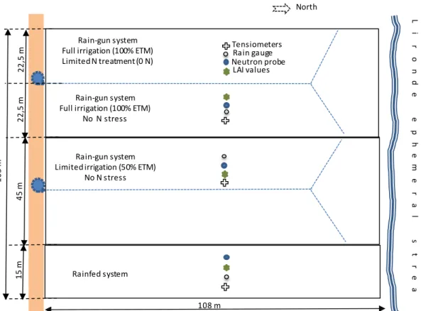
The experiments were described in previous papers focusing on water (Mailhol et al, 1997; Khaledian et al., 2009; Mailhol et al, 2011) or nitrogen management (Mailhol et al., 2001; Khaledian et al., 2011). The experimental domain of Lavalette is divided in several plots with different designs between seasons (Fig. 1 shows an example for 2012), supporting dedicated treatments, the size of which may vary from a few hundreds to a few thousand square meters. The treatments are either irrigated by sprinklers, by a travelling rain gun system or by subsurface drip irrigation (SDI). Irrigation scheduling was based on tensiometer readings or some time using PILOTE itself. Water application depths ranged from 25 to 35 mm by the sprinkler systems and between 5 and15 mm by SDI. From 2011 the limited irrigation treatments consisted in stopping irrigation at the end of July. A non-fertilized treatment (0N) has in most cases been conducted for the evaluation of soil mineralization and a rain-fed treatment (RF) to calculate the irrigation water productivity (Mailhol et al., 2011). Neutron probes were used to monitor soil water content in the middle of each plot, always complemented by a series of tensiometers. Manual rain gauges were also installed in the vicinity of neutron probes to accurately estimate the local rainfall and irrigation amounts. LAI measurements were performed, at least weekly, throughout the cropping seasons using the LAI probe (LAI-COR-2000 Plant Canopy Analyzor LAI-meter). Several sub-plots (most often, seven) of 2-3 m2, located in the vicinity measurement sites, were harvested after maturity to assess grain yield and biomass production and to assess nitrogen content in plants (leaves, stems and grains) according to the Kjeldahl method.
The experiments conducted on Lavalette were mainly devoted to irrigation management, which is the reason why N in plant is only known at harvest dates, to verify if the yield gap is not due to a lack of nitrogen. The corn season 1999 was essentially focused on the fate of nitrogen under different irrigation systems (Mailhol et al., 2001) but unfortunately only one couple of total dry matter and Nitrogen in plants (TDM, Np) is available during the cropping season, in addition to that obtained at harvest.
The profiles of nitrogen concentration in the soil solution near the measurement sites were characterized before sowing and after harvesting from the soil to surface to 1.5 m depth, with step of 30 cm.. The technique of the averaged soil sample consisting in mixing 3 or 4 soil samples collected with an auger at each step is explained in detail in Khaledian et al. (2011). The N applications were only measured with precision from 1999 to 2007, using plastic bowls around the measurements sites. Outside this period the precision on the N amounts depends on the performance of the spreading machine.
By the end of each growing season, crop residues were buried at shallow depths during tillage. Note that oat was sown on DOY285 in 2012, as a cover-crop for FIC13. For the summer crops, the nitrogen applications were immediately followed by irrigation, which was not the case for winter crops (durum wheat). Finally, it is noteworthy that drainage is most likely to occur during autumn as a result of typical strong rainfall events during this period of the year in Montpellier, with occasional nitrogen losses by lixiviation.
3. Model calibration
The first step of the calibration is devoted to CM, the parameter involved in the mineralization process. Then calibration will be detailed for the parameters involved in the N plant uptake process and for those that control crop yield.
3.1. Calibration and validation of the mineralization module
The nitrogen amount resulting from the soil mineralization was obtained as proposed by Khaledian et al. (2011) from the 0N treatments. During each experiment, the tensiometers (not shown here) indicated no drainage, thus no lixiviation, and the conditions were not favorable for denitrification. CM was thus (Section 2.2.4, Eqs.12-13) the only parameter to calibrate. The volumetric organic matter content OM of about 1.5 % and soil pH of 7.5 are the soil characteristic values considered for our experimental site. Consequently a CM value of 0.075 yields a mineralization rate of 0.75 kg ha-1
d-1, in agreement with that found by Nemeth (2001) at Lavalette. The reference and minimum temperatures for mineralization were respectively 20°C and 5°C. This parameter set (CM=0.075, TMr = 20°C and Tmin = 5°C) yields in average 100 kg ha-1 of total mineralization, a value generally found in literature (e.g. Desvigne, 1993; Mary and Recous, 1994; Campbell et al., 1984; Quemada and Cabrera, 1997).
The validation of this parameter value can be performed independently from PILOTE-N and thus may immediately follow calibration.
Since plant transpiration Tp is required to derive in Eq.12, PILOTE can be used with the daily values of rainfall, irrigation. Tp is calculated using Eqs. 1 to 5 and the measured LAI values for a given "light nitrogen" LN (or "zero-nitrogen" 0N) treatment. Note that irrigation was not limited and consequently one can assume that there was no water stress.
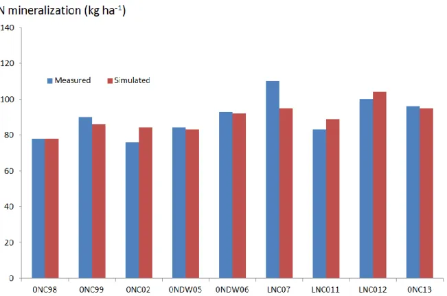
Mineralization was reasonably simulated as shown in Fig.2, except in 2007 where it is noticeably underestimated (95 vs. 110 kg ha-1). It will be further strengthened by model simulations conducted during the inter-cropping season.
3.2. Calibration of the plant nitrogen uptake and grain yield
The calibration process in this case concerns x1 and x2, the shape parameters for the N plant demand (Eq.16), then Ka of Eq.17, and finally aN involved in the estimation of the HI harvest index required for the grain yield calculation when the N stress is higher than the water stress.
3.2.1. Calibration for corn
The process starts with the calibration of x1 and x2. The plant nitrogen content was not monitored during the cropping cycle on any unstressed corn treatment, except for FIC99 (cf. Table 1) with only two measurements of (TDM, Np) pairs. To overcome this limitation, the shape parameters x1 and x2 were calibrated based on the shape of the critical curve of the N plant demand formulated by Justes and al. (1994; 1997) and Plenet (1995). Using this critical curve (%Np = acritTDMb crit, where acrit and bcrit are dimensionless empirical parameters) allows generating a series of (TDM, Np) pairs. Exploiting the analogy between Eq.1 and Eq.14, the fitting method used in Mailhol et al. (1997) and Khaledian et al. (2009) to obtain the shape parameters of the LAI curve vs. temperatures (Eq.1) was also used to obtain the x1 and x2 parameters. A distinction between corn cultivars is pointed out in this new formulation by specific values of PCNDmax and TDMpot (Eq.14), assuming the values of x1
and x2 depend on the crop, not on the cultivar. The values of x1 and x2 were 0.45 and 1.5 respectively.
The values of PCNDmax and TDMpot were set to 300 kg ha-1 and 23 Mg ha-1 for the SAMSARA cultivar. For the other late corn cultivar (PR35Y65) the potential TDM value is set to 30 Mg ha-1 (e.g. Lamm and Trooien, 2005; Couto et al., 2013) and that of PCNDmax to 380 kg ha-1, for a grain yield of GY=17.5 Mg ha-1 (see Table 1). In absence of dedicated field experiments, the same harmfulness was assumed for the water and nitrogen stresses and = N = as proposed by Khaledian et alfor field crops (corn, sorghum and wheat).
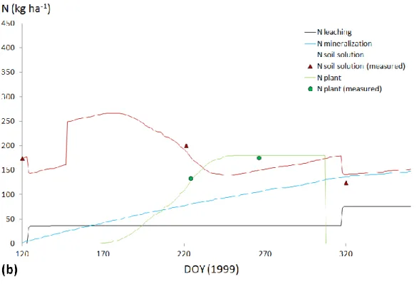
The parameter Ka (Eq.17) was calibrated from the FIC99 treatment, resulting in a value of 2.5, validated then on RFC99. It is shown in Fig.3a and b that this value allows a correct estimation of the N contents in both plant and soil. It is noteworthy that N soil storage is also reasonably simulated at the beginning of the cropping cycle and after the rainy periods from the end of September to the half of November (DOY= 313) for FIC99.
Parameter aN was calibrated on the grain yield of 0NC99 because TDM (12 Mg ha-1) of this treatment is perfectly simulated. Its value (0.15) was found slightly higher than that of aN (aN = 0.12 in Khaledian et al., 2009) used to account for the effect of water stress on the harvest index, then in turn on grain yield (Eq.21).
3.2.2. Calibration for durum wheat
The crop parameters for durum wheat were drawn from Khaledian et al. (2009) for the unstressed N treatment. Under our experimental layout the potential value of TDM was not reached. Consequently, the PCNDmax and TDMpot values were drawn from literature and their values were assigned respectively to 280 kg ha-1 and 17 Mg ha-1 (Casals, 1996; ARVALIS, 2016). The calibration of the shape parameters was conducted similarly to the corn case, based on the N critical curve proposed by Justes et al. (1994), obtaining 0.8 and 1.4 for x1 and x2, respectively. Adopting the same assumption for, the value of Ka equal to 3 was found on DWLI05 to significantly improve both the prediction of N content in the plant and that of grain yield, with the same value of aN for corn (0.10).
The PCNDmax value was set to 250 kg ha-1 associated to TDMpot of 19 Mg ha-1. These values are proposed by ARVALIS (ARVALIS 2012), a French institute which conducts studies on field crops and other plant species. Parameters x1, x2 and Ka were calibrated with the same method as for corn and durum wheat. The values for x1, x2 were found equal to 1 and 2, respectively and Ka was 4, from the FIS04 treatment. Nitrogen content in the plant was reasonably simulated. The highest gap between simulated and observed values was obtained for RFS03, respectively 110 vs. 95 kg ha-1 (not presented). N soil storage over the entire root zone (1.5 m deep as average depth for sorghum) at harvest was acceptably simulated for RFS03 (110 vs. 129 kg ha-1) and for RFS04 (112 vs. 110 kg ha -1), compared with the irrigated treatments LIS03 (67 vs. 99 kg ha-1) and FIS04 (77 vs. 50 kg ha-1)
4. Model validation
4.1. LAI and Soil Water Reserve (SWR)
Many examples of model performance regarding LAI and the soil water reserve (SWR) simulations are presented in previous articles implying PILOTE where N is not a limiting factor. The ability of PILOTE-N to simulate not limited conditions both for water and nitrogen is thus little surprising. By contrast, the differences modeled between a full fertilized and a 0N treatment, both subject to the same irrigation strategy, should be pointed out (Fig. 4). Indeed, the SWR variation is substantially weak along the cropping cycle for 0N, with consequently, a lower Ce value (the coefficient of efficiency of Nash and Sutcliffe, 1970).
LAI for 0N and LN treatments which ranged from 1.6 to 3.1, are not very well simulated, with performance criteria of 0.595, 0.34 and -0.18 for R2, the Root Mean Square Error (RMSE) and the Mean Biased Error (MBE), respectively. The negative value for MBE attests that LAI is somewhat underestimated by PILOTE-N. These same criteria are much better for the whole set of treatments (R2 = 0.934 ; RMSE = 0,24 ; MBE = -0.01).
4.2. Mineralization and lixiviation during the intercropping period
The specificity of the lixiviation process adopted in PILOTE-N which could be considered as the weakest link in the model merits a peculiar attention. Because no parameter involved in this process required any calibration, this section is first dedicated to evaluating mineralization during the intercropping period. But overall, we focus on the lixiviation component of the model under different
The ability of PILOTE-N to correctly simulate N leaching implies thus the correct simulation of drainage, in addition to N plant uptake and soil mineralization processes. Generally, substantial drainage occurs during intercropping periods. We recognize that a specific protocol involving the installation of lysimeters for evaluating drainage and N leaching during intercropping period would have been necessary. However, one can attempt to show that leaching can be validated, on the basis of N soil storages (Nsoil) leaning on a few plausible hypotheses regarding mineralization, described in the following.
4.2.1. Mineralization
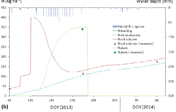
We have to prove first that mineralization during intercropping periods is well simulated, before considering the leaching process itself. For that, we have to seek periods without rainfall that could induce drainage. When looking at Fig. 5, one can assume that mineralization during the intercropping period is satisfactorily simulated on the basis of simulated and measured Nsoil. Mineralization is significantly lower for FIC13 (Fig.5b) than for 0NC13 (Fig.5a) because the soil water profile was much more depleted for FIC13 than for 0NC13 at the end of the cropping season (not presented), a consequence of the nitrogen deficit that reduces LAI and consequently transpiration, as shown in Fig.4b. Mineralization is low from DOY300 to DOY420 due the weakness of temperatures during winter.
4.2.2. Leaching
Some contrasted examples of N leaching during intercropping periods are presented in what follows, starting with heavy drainage conditions. Such conditions occurred for FIC97, FIC98, FIC12 and FIC13 for corn and also twice for durum wheat, for which experiments DWLI05 and DWLI06 are fairly well simulated. FIC97 and FIC98 received 613 mm of rainfall during the cropping season, resulting in a simulated drainage of 266 mm. FIC12-13 received 710 mm rainfall for a simulated drainage of 392 mm. Fig.6 shows that Np and Nsoil are correctly simulated, which implies that leaching also is reasonably simulated for the corn case.
Durum wheat, generally sown in autumn in South-East of France, can be affected by substantial rainfall periods inducing drainage and leaching risks, as presented in Fig.7. Rainfall during 2004-2005 and 2004-2005-2006 experiments was 820 mm (from DOY320 to DOY720 e.g. end of 2004-2005) and 366 mm from DOY320 to DOY570 e.g. end of July 2006), respectively, with a simulated drainage of 249 and 166 mm, respectively. Still hypothesizing that mineralization during the cropping cycle is well simulated, based on the fact that Nsoil is correctly predicted, N leaching (occurring mainly outside the growing period) is then also well simulated.
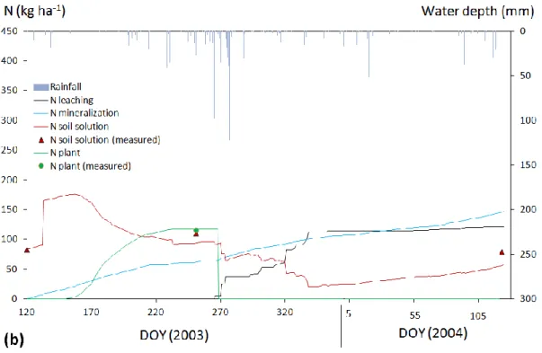
The intercropping periods 2002-2003 for corn and 2003-2004 for sorghum were particularly rainy. Indeed, rainfall and simulated drainage were 804 and 547 mm, respectively, for 2002-2003 and 1290 and 660 mm, respectively, for 2003-2004. PILOTE-N simulates Nsoil and Np reasonably under such heavy drainage conditions (Fig.8) hypothesizing that mineralization during intercropping season is correctly predicted.
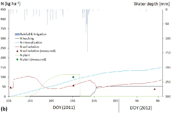
Moderate drainage conditions were also observed during the experiments. The intercropping season 2011-2012 raises questions since Nsoil measured at the end of March (DOY456) is substantially overestimated by the model as shown by Fig.9. For 2011-2012 the rainfall was 305 mm from DOY 273 to DOY 334, while simulated drainage, predicted to start on DOY 307 equals 174 mm for FIC11 and 260 mm for 0NC11. One can notice that Nsoil at the end of the drainage period (around DOY 310) has the same value of that measured at the end of March 2012 (DOY 446). This overestimation of Nsoil by the model on DOY 446 could result from the immobilization process probably more efficient or more noticeable under un-cropped soil with substantial crop residue conditions than under these previously presented. Indeed, the N amount (around 30 kg ha-1) consumed by the microbial fauna during the assumed process seems a realistic value according to Mary et al. (1999). Under moderate drainage and leaching conditions, a possible failure of the simple mineralization module is thus highlighted. This example points out the difficulty of predicting the N balance even during the intercropping season on un-cropped soil without involving an efficient crop residue model. However, our main objective is the prediction of the N balance during the cropping season assuming that Nsoil few days before sowing is required.
4.3. Model evaluation along the 14 years of experiments
Fig.10 and 11 refer to the soil N storage at the end of the cropping cycle, to N plant uptake and to crop yields. The N soil storage (Fig.10a) exhibits some discrepancies confirming that some phenomena are not always identified or captured. That is particularly the case when the N balance evaluated from measurements cannot be closed without any robust explanations (no drainage, no favorable conditions for volatilization or denitrification). The numerical criteria such as the coefficient of determination (R2) and the root mean square error (RMSE) are satisfactory for Np and yields, while the mean bias error (MBE) with values of 0.04 and 0.03, respectively, does not attest significant overestimation. R2 and RMSE values are noticeably lower for Nsoil, with MBE = 3.03. This can also be due to a lack of precision regarding N applications, as in 1998 for the rain-fed treatment where the N application were only estimated. But, as discussed above for the sorghum
N plant uptake (Fig.10b) is well enough simulated even for the 0N treatments such as for instance in 1999 (83 vs 90 kg ha-1) or for the light N treatments, while this quantity is often overestimated by most of the crop models as shown in Nemeth (2001).
Total dry matter and grain yields are rather well simulated, as attested by Fig.11, even if the later also shows some overestimations of TDM on the 0N treatments, as for example for 2012 (12.8 vs. 14.3 Mg ha-1) and 1998 (10.3 vs. 11.5 Mg ha-1).
5. Discussion
In the present work, we did not intend to add another crop model to literature but rather to enhance and complement an existing one, PILOTE, which has been used for years for irrigation management and now tackles joint irrigation and N-fertilization management. The scientific interest of this work is in fulfilling the challenge to maintain the user-friendly and operational character of PILOTE, augmented with nitrogen management facilities. From the acceptability of the results obtained for a contrasted climatic series over 14 years, one can consider that our objective is reached. Indeed, we can say that "a good representation of reality" (Affholder and al., 2012) is proposed by this model since the predictions are performed with "acceptable accuracy and precision", as formulated by Loague et al. (1991).
PILOTE-N stands apart from most crop models by ruling the potential cumulative N plant demand by a logistic-like curve similar to that used for the increase of LAI with time. In addition, the shape parameters of this curve allow its application to different cultivars from the same species, as shown for the corn case. Although empirical, the role played by these parameters in the N plant uptake process is well identified. Indeed, the period where the N plant demand is the highest can easily be advanced or the delayed by decreasing or increasing x1. A supplementary degree of freedom exists in the form of the required maximal N plant demand for the desired cultivar, a value generally proposed in literature, which serves as a scaling parameter for the curve.
The concept of successive soil water reservoirs of PILOTE is extended, in PILOTE-N, to nitrogen. As for water, N is taken up by plants according to a quasi-lumped model (using two variable-depth reservoirs) in which the soil is not multilayered, a true specificity amongst models developed to simulate the N fate. This quasi-lumped approach implicitly accounts for the compensated root water and nutrient uptake, a phenomenon not always well simulated by multilayered crop models (Simunek and Hopmans, 2009; Albasha et al., 2015). The allocation from the common pool to the different plant organs is not based on the source-sink principle as in some crop models. In PILOTE-N (as in PILOTE), LAI is not derived from TDM (the common pool for models based on the allocation
principle) but simulated based on temperature accumulation (i.e. thermal time), before the current LAI value is used to calculate the TDM increase of the same day. Although not pointed out in the case of field crops, it is all the same possible to discriminate the impact of water or N stresses on the grain yield via the adequate harvest index formulations. Thus, despite its simplicity, our modeling approach offers some flexibility.
Some weaknesses of PILOTE-N are attested by occasional gaps between measured and predicted N soil storages after a rainy period during the inter-cropping season, could result from the fact that leaching is simulated based on a very rough approach. Indeed, the capacitive approach here used is very far from that used in LIXIM (Mary et al., 1999) in which N leaching is simulated according to the Burns (1980) model and where a peculiar attention is devoted to the role of crop residues. The authors recognize that a specific protocol should have been implemented for validating both mineralization and lixiviation during intercropping seasons, as proposed by Mary et al. (1999). Nevertheless, despite the assumption adopted regarding mineralization, the simulated N soil storages at the end of rainy periods (beginning of winter), associated with substantial drainage, do not differ a lot from the measured ones. The origin of the evoked gap between simulated and measured N soil storage at the end of the period 2011-2012 could result from losses by immobilization, a process requiring the use of an efficient crop residue model. The latter has been developed in the frame of this research. Because not validated yet it is not presented here. Under our experimental conditions, drainage rarely occurs during the cropping season more especially for summer crops. However, we compared simulations obtained with PILOTE-N and PILOTE (not shown here) to evaluate the added value of the N module. We noticed that PILOTE-N gave better yield predictions under drainage conditions than PILOTE. That could strengthen, in a way, the credibility of the nitrogen lixiviation simulated by the model as for the DW case 2008-2009 and that of corn in 2008 as further explained. Note that the variable-depth compartments used for the N balance calculation may appear little justified due to the fact that, at the beginning of the cropping cycle, the N plant demand is low and can be compensated by mineralization. However, in case of heavy rain conditions, a substantial N amount can leach out of the first compartment to supply totally or partially the second one, which could impact the N plant uptake conditions: this is a process representation specific to the model. Although the different mineralization models proposed in the literature use similar factors (mainly soil water content, temperature and soil properties) as those proposed in PILOTE-N, the latter is more simpler owing to its limited objectives (residue decomposition not taken into account yet) and still gives acceptable results by using air temperature instead of soil temperature. Mineralization is
drainage period from DOY 250 (2013) to DOY 90 (2014) due to the absence of heavy rainfall, confirms the ability of the model to properly simulate mineralization during the inter-season, the N soil storages being correctly predicted as shown by Fig.5.
LIC of 2007, 2011, 2012 and 2013 highlighted the pertinence of a reduction in N application for water-scarce conditions attesting that nitrogen savings are possible when the initial N soil storage before sowing is known. A case that deserves dedicated attention is the rain-fed treatment of 2008. This cropping season with corn, was not selected because N in the plant was not measured. But it was sufficiently rainy (235 mm on the cropping cycle) to point out the effect of a reduction in N inputs (37 kg N ha-1 only at sowing) responsible for the low final grain yield, unlike other rain-fed treatments analyzed in this article. The fact that PILOTE substantially overestimates the corn yield (7.3 vs. 4.0 Mg ha-1) compared with PILOTE-N (4.3 vs. 4.0 Mg.ha-1) highlights the difficulty to manage efficiently both water and nitrogen, since the rainfall forecast is not possible for a farmer. For the durum wheat case, the application of PILOTE-N allowed noticing that the low yield value for the 2008-2009 cropping season was due to N leaching, whereas PILOTE substantially overestimated the yields. This statement pleads in favor of the identification of an efficient N management strategy using a modeling approach such as that proposed by PILOTE-N.
Due to the absence of a treatment both full irrigated and full fertilized, and for which a series of (TDM, Np) pairs would have been monitored along the cropping cycle, the shape parameters (x1, x2) for the cumulative nitrogen plant demand were calibrated on the N critical curve proposed by Justes et al., (1994). This should ensure a correct simulation of Np along the cropping cycle (in adequacy with TDM) and not at harvest only. But we recognize that the lack of (TDM, Np) pairs measured during the growing phase (except for FIC99 and RFC99) may raise criticisms. More precisely, a model run with an inadequate parameter set (x1, x2), can result in a good prediction of the (TDM, Np) pair at harvest but the temporal coherence would be poor and significant gaps between predicted and observed values would appear during the cropping season, especially for Np. It can be noticed that, in average, 85-90% of the final nitrogen plant consumption is reached few days after the maximal LAI value is reached, with the parameter set (x1, x2) calibrated by the proposed method.
As evoked in introduction, PILOTE-N is an interesting tool for analyzing abiotic stresses. That is especially obvious when comparing treatments both fully irrigated and little fertilized (LN11, LNC12) with rain-fed treatments (RFC11, RFC12) also little fertilized, with similar moderate initial N soil storage. As shown on Table 1, the corn yields of the rain-fed treatment are noticeably lower than the little fertilized ones attesting thus the preponderance of water stress on N stress. When disconnecting the N module (passing from PILOTE-N to PILOTE) the yields of the rain-fed treatments were very well simulated which means that water stress is responsible of the weakness of
the yields despite a very light fertilization. The condition to correctly account for such situations is that N stress should not appear before water stress in time. This condition is met due to the shape of the N plant demand and by the fact that the latter is reduced within the water stress period. The necessity to reduce fertilization under limited water conditions is clearly shown by this analysis, and the water management under such conditions could be performed using PILOTE only.
There is no question that a sound sensitivity analysis would merit to be performed. It was conducted by Khaledian et al. (2009). It revealed that PILOTE was sensitive to initial soil water content more especially for the rain-fed and the little irrigated treatments. A similar statement can also be proposed to PILOTE-N regarding the initial N soil storage for the limited N treatment. Nitrogen plant uptake and yields are little sensitive to Ka, in particular on the limited N treatments because plant cannot take up more N than offered by the soil. On the no limited N treatments, a 25% variation of Ka gives a variation of N in plant lower than 5% at harvest. N in the plant is little sensitive to the shape parameters ruling the curve of the potential N demand. For instance a 25% variation of the shape parameters results in variation of N in plant lower than 5% at harvest. The impact on TDM is higher on the N limited treatments. A 25% variation of the shape parameters results in a TDM variation at harvest lower than 7% in average and lower than 3% for moderate or full fertilized treatments. This sensitivity of TDM and that of N in plant to the shape parameters is a little higher at the beginning of the cropping cycle and more especially with respect to x1 because this parameter allows to advance or to delay the period during which plant requires the highest N amount.
Of course the sensitivity of GY to aN is essentially highlighted on the limited N treatments. This sensitivity can be considered moderate. For instance, when aN decreases from 0.14 to 0.12, GY increases from 6.0 to 6.2 Mg ha-1and decreases by 0.2 Mg ha-1 when a
N increases from 0.14 to 0.16 on treatment 0NC11. A similar model behavior can be observed on the other treatments.
At this stage, the convenience of using such a tool (written in FORTRAN), merits to be highlighted. As written in Khaledian et al. (2009) for PILOTE, most of the model parameters can be measured or derived from literature. Only the shape parameters (, of LAI and which is dedicated to simulate the impact of the water stress conditions on both on LAI and TDM, have to be calibrated for the case of a new crop. Regarding PILOTE-N, the only parameters to calibrate are x1, x2 and Ka. Finally, specific treatments are needed for the calibration of aN, parameter dedicated to the harvest index, for crops having a same sensitivity to water and to N stress.
In order to correctly simulate Np for the full fertilized N treatment Nemeth (2001) and Poch- Massegù (2012) have modified the initial parameters governing the N plant uptake of STICS in the Mediterranean context. Since highly predictive crop models do not exist, it is advantageous to have a
model easy to calibrate, to run in optimization scenarios or to update within data assimilation techniques, which are forthcoming works with the PILOTE model (e.g. the Optirrig tool for the generation, analysis and optimisation of irrigation scenarios, possibly running with nitrogen management options, Cheviron et al., 2016). For instance, the SPAD-502 chlorophyll meter, (Bulloc et al. 1995) an apparatus allowing the N monitoring in the plant, can be used to update specific parameters (which involved in the N plant uptake process) of the N module. For analysing the nitrogen stress, it would probably be more interesting than an apparatus such as the LAI2000 based on the light interception, and which does not provide information about the percentage of photosynthetic active mater. This could initiate further researches for justifying the fact that LAI is little under estimated by PILOTE-N for the 0N treatments while SWR is rather well simulated for these treatments.
6. Conclusions
The objective of this work was to propose a convenient tool for predicting the impact of a reduction of nitrogen inputs on the crop production. It is reached since both N in the plant and crop yields are correctly simulated under both sub-optimal water and nitrogen applications, for a long climatic series (1997-2013). This performance merits to be pointed out for a model whose empirical concepts could be criticized for their simplicity and weak predictive abilities. Moreover, PILOTE-N stands apart from most crop models by its originality, since its main components or equations are not derived from existing models, unlike most recent crop models.
This PILOTE version is not a research tool compared with more sophisticated crop models such as STICS (Brisson et al. 1998), developed by a group of agronomists supported by modellers, each one being a specialist of one of the processes embedded in the whole model. Instead, PILOTE is a convenient tool with limited objectives, which allows easier identification of the different sources of uncertainties that affect the nitrogen balance along a cropping cycle.
This paper is mainly focused on the application of PILOTE-N on the experimental site of Lavalette (Montpellier SE of France). The results obtained in this context encourage testing it under other agro-climatic conditions.
A substantial database as that of Lavalette, makes possible the validation of different modelling approaches. The present development of PILOTE-N should initiate studies devoted to the comparison of different modelling approaches in the domain of crop modelling. In the frame of such a work, the pertinence of a given formulation rather than another one for solving a specific question would be soundly analysed.
For a variety of reasons, this PILOTE version can be more especially useful for practitioners or economists for evaluating the impact of input reductions such as water and fertilizers under contexts where the accessibility to data is generally limited.
Aknowledgments
The research unit US49 of the CIRAD institute (Centre of Montpellier) is gratefully acknowledged for performing all nitrogen content analysis.
References:
Albasha, R., Mailhol, J.C, Cheviron, B., 2015. Compensatory uptake functions in empirical
macroscopic root water uptake models – Experimental and numerical analysis. AGWAT 155: 22-39.
Affholder, F., Tittonell, M., Corbeels, M., Motisi, Tixier,P., Wery, J., 2012. Ad Hoc
Modelling in Agronomy: What have we learned in the last 15 years. Agron. J. 104:735-748. Agostini F, Tei F, Silgram M, Farneselli M, Benincasa P, Aller MF., 2010. Decreasing nitrate
leaching in vegetable crops through improvements in N fertiliser management. In: Lichtfouse, E. (Ed.), Genetic Engineering, Biofertilisation, Soil Quality and Organic Farming (Sustainable Agriculture Review, 4). SpringerScience + Business Media B.V. pp. 147 – 200.
Allen, R. G., Pereira, L. S., Raes D., Smith, M., 1998. Crop evapotranspiration: Guidelines for computing crop water requirements. Irrig and Drain. Paper 56 FAO, Rome. 300 pp.
ARVALIS-Institut du végétal, 2012.’’Les conduites des cultures : choisir sorgho’’ 2012. 60-72p. ARVALIS-Institut du végétal, 2016.’’Fiche cycle du blé dur’’ : info.,19-01-2016.
Barakat, M., Cheviron, B., Angulo-Jaramillo,R., 2016. Influence of the irrigation technique and strategies on the nitrogen cycle and budjet. A review, Agric. Water Manag. 178 225-238. Brisson, N., Mary, B., Ripoche, D., Jeufroy, M.H., Ruget, F., Nicoullaud, B.,
Gate, P., Devienn-Barret 1998, F. Antonioletti, R., Durr C., Richard G., Beaudoin, N., Recous, S., Tayot, X., Plenet, D., Cellier, P., Machet, J.M., Meynard, J.M., Delécolle, R., 1998. STICS: a generic model for the simulation of crops and their water and nitrogen balances. Theory and parametrisation applied to wheat and corn. Agronomie, No 18, 311-346.
Brisson, N, Gary, C., Justes, E., Roche, R., Mary, B., Ripoche, D.,Zimmer, D., Sierra, J.,Bertuzzi, P., Burger, P., Bussière, F., Cabidoche , Y.M., Cellier, P., Debaeke, P., Guadillère, J.P., Hénnault, C., Maraux, F., Seguin, B., Sinoquet, H., 2003. An overview of the crop model