Essays on asset bubbles and secular stagnation

(1)

HAL Id: tel-02421223

https://tel.archives-ouvertes.fr/tel-02421223

Submitted on 20 Dec 2019

HAL is a multi-disciplinary open access archive for the deposit and dissemination of sci-entific research documents, whether they are pub-lished or not. The documents may come from teaching and research institutions in France or abroad, or from public or private research centers.

L’archive ouverte pluridisciplinaire HAL, est destinée au dépôt et à la diffusion de documents scientifiques de niveau recherche, publiés ou non, émanant des établissements d’enseignement et de recherche français ou étrangers, des laboratoires publics ou privés.

Mathieu Boullot

To cite this version:

Mathieu Boullot. Essays on asset bubbles and secular stagnation. Economics and Finance. Université Panthéon-Sorbonne - Paris I, 2019. English. �NNT : 2019PA01E007�. �tel-02421223�

(2)

UFR 02 Sciences économiques

Laboratoire de rattachement : Paris Jourdan Sciences économiques

THÈSE

Pour l’obtention du titre de Docteur en sciences économiques Présentée et soutenue publiquement le

15 Mars 2019 par

Mathieu Boullot

Essays on Asset Bubbles and Secular Stagnation

Sous la direction de:

Bertrand Wigniolle, Professeur, Université Paris 1 Panthéon-Sorbonne, Paris School of Economics Membres du jury:

Thomas Seegmuller Rapporteur, Professeur, Aix-Marseille School of Economics, CNRS Jean-Baptiste Michau, Rapporteur, Professeur, Ecole Polytechnique

Eleni Iliopulos, Examinatrice, Professeure, Université Paris-Saclay, CEPREMAP

Jean-Bernard Chatelain, Examinateur, Professeur, Université Paris 1 Panthéon-Sorbonne, Paris School of Economics

(3)

(4)

Remerciements

J’aimerais tout d’abord remercier mon directeur de thèse, Bertrand Wigniolle. Sans son soutien, ses encouragements et ses conseils, je n’aurais pu achever cette thèse, ni proﬁter pleinement de l’expérience. Plus particulièrement, merci Bertrand d’avoir supporté mes idiosyncrasies et mes doutes, de m’avoir décidé à enﬁn clôre cette thèse, et d’avoir été un directeur très humain et compréhensif.

Je tiens ensuite à remercier toutes les personnes, personnels enseignants, administratifs ou étudiants, que j’ai eu l’occasion de rencontrer à la Maison des Sciences Économiques, à l’Universtié de Bielefed, à l’Ecole d’Economie de Paris, et aux divers séminaires et conférences auxquels j’ai eu la chance de participer. Le présent travail a bénéﬁcié de nombreuses discussions et commentaires. Je remercie également l’ENS Paris-Saclay, et tout particulièrement Jean-Cristophe Tavanti, de m’avoir proposé un poste d’ATER le temps de terminer cette thèse.

Merci aux membres de mon jury de thèse, Jean-Baptiste Michau, Eleni Iliopulos, Jean-Bernard Chatelain, et tout particulièrement à Thomas Seegmuller, qui a suivi l’avancement de cette thèse dès mon mémoire de Master 2, et m’a aidé continuellement à améliorer mes travaux.

On dit qu’entrer en thèse, c’est aussi commencer une analyse. Merci à tous ceux qui ont eu à supporter, et ont su m’aider à supporter, mes doutes et questionnements durant ces cinq ans. Je pense en particulier à Guillaume, Sandra, Giorgio, Antoine, Swann et Johan. Et merci également à tous les autres, dont la liste serait trop longue à énumérer ici.

Un grand merci à toute ma famille, et en particulier à mes parents, Alain et Brigitte, sans qui je n’aurais eu l’opportunité d’arriver jusqu’en thèse, et à mes grand-parents, Eugène et Adrienne, pour m’avoir permis de travailler à cette thèse hors de l’agitation de Paris, et à proximité de l’océan! Un grand merci également à mon frère, Romain, pour son soutien constant – ainsi que le yucca qui a embelli mon espace de travail.

Enﬁn, je tiens tout particulièrement à remercier Arwa, sans qui ce projet n’aurait pu aboutir.

(5)

Introduction

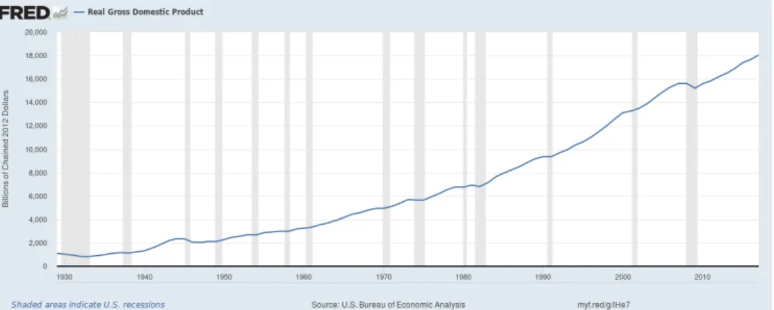
The graphic below plots the real gross domestic product (RGDP) of the United States since 1929. Strikingly, over the long run, even the ﬁnancial crises of 1929 and 2008 are almost indistinguishable.

Figure 1: US RGDP, Billions of Chained 2012 Dollars, from 1929 to 2017. Source: Bureau of Economic Analysis

Yet, to quote the famous words of John Maynard Keynes, "in the long run, we’re all dead". Even if it was a minor event from a (very) long run perspective, the Great Recession of 2008 was a painful experience for dozens of millions of people.

Over the course of two years, the US unemployment rate nearly doubled, and it remained elevated for almost ten years. Even now, the growth rate of nominal wages is still low and the employment-population ratio didn’t recover: some discouraged workers decided to exit the labor force during the crisis, but didn’t re-enter the labor market after the crisis.

(9)

Figure 2: US Unemployment Rate: 20 years and over, %, from 2000 to 2019. Source: Bureau of Labor Statistics

As of today, the US economy appears quite strong. However, the next crisis might already be looming on the horizon: according to the NBER1_{, the average duration between two troughs is 70} months in the US since 1945. The last expansion began in June 2009: most than 100 months have passed since the last trough.

And the US economy is unprepared to yet another recession. The Great Recession lasted for almost 10 years despite large-scale programs aimed at supporting aggregate demand (i.e zero nominal interest rates, quantitative easing, stimulative ﬁscal policy ect.). But, since public debt has dramatically increased during the crisis, but it wasn’t reduced during the expansion, the US ﬁscal capacity is strongly impaired.

Figure 3: US Public Debt / GDP ratio, %, from 2000 to 2019. Source: Saint Louis FED

Furthermore, both the federal funds rate (the nominal interest rate) as well as the real interest rate remain close to zero: there isn’t much room for conventional monetary policy either.

(10)

Figure 4: Federal Funds Rate, %, from 2000 to 2019. Source: Board of Governors of the FED system

Thus, if another crisis of the same caliber were to hit the US during the next decade, the situation could quickly become out of control. Therefore, it is more crucial than ever to understand the roots of the 2008 crisis, and hence to determine how to prevent such crises to happen again.

According to Summers (2013) and Krugman (2013), there are two key notions to understand the 2008 crisis: secular stagnation and asset bubbles. I’ll brieﬂy develop those notions, and then provide a narrative of this "bubble-secular stagnation" theory of the 2008 crisis.

The price of an asset includes a bubble when it exceeds the fundamental value of this asset, which is equal to the sum of discounted ﬂows of future dividends. Historical examples include the South Sea bubble (England, 18th century), the Tulip Mania bubble (Netherlands, 17th century), or the recent Dot Com bubble (US, 2001). Usually, those bubbly episodes involve speculative behaviors: investors start to accumulate the bubbly asset because they expect to realize high capital gains. Seemingly unrelated, the secular stagnation hypothesis traces back to Hansen (1939). Although Keynesian, demand-led, recessions are usually thought of as temporary, i.e the typical recession in the US lasts around ﬁve years,Hansen (1939) speculated that, absent adequate aggregate demand management policies, demand-led depressions could be very persistent or even permanent.

The narrative of the secular stagnation - asset bubble theory goes as follows. For decades, aggregate demand in the US has been on a downward trend because of divers structural changes2_. However, the mortgage-backed securities (MBS) bubble kept aggregate demand from falling "too low": the central bank still had some leverage over the economy. But this bubble imploded shortly after Lehman Brothers went bankrupt in 2008: investors realized that those MBS weren’t as safe

2_{E.g lower rates of productivity and population growth, an increasing demand for USD-denominated assets by}

emerging economies, sky-rocketing income and wealth inequalities, a higher share of intangible capital vs physical capital etc.

(11)

as they sought, but rather exposed to the housing market that had just crashed a few months ago. This led them to re-evaluate a large fraction of those assets as worthless. This sudden and permanent shock to the supply of assets drastically reduced aggregate demand. It couldn’t be fully oﬀset by the FED because of the binding Zero Lower Bound (ZLB). Thus, the US economy entered a period of secular stagnation. Among others, Caballero et al. (2008) provide some stylized facts consistent with this interpretation of the events.

This thesis consists in three chapters, each analyzing a particular aspect of the asset bubble - secular stagnation theory. The first paper, "Asset Bubbles and the Income Distribution", which is based on my Master’s thesis, focuses on the emergence of asset bubbles. More specifically, it analyzes from a theoretical point of view whether a high concentration at the top of the income distribution promotes or prevents the emergence of asset bubbles. I show that a high level of inequality promotes the emergence of asset bubbles whenever asset bubbles are illiquid and/or financial markets are arbitrage-free; a contrario, a low level of inequality promotes the emergence of asset bubbles when those bubbles are liquid and liquid assets pay a premium under illiquid assets. The second paper, "Secular Stagnation, Liquidity Trap and Asset Bubbles", deals more directly with theSummers(2013)-Krugman (2013) hypothesis: it analysis under which circumstances asset bubbles are expansionary in the long run in a New Keynesian model that includes capital. I show that secular stagnation is a necessary, but not sufficient, condition for asset bubbles to be expansionary. Indeed, asset bubbles raise a trade-off between a positive demand-side effect vs a negative supply-side effect. The demand-side effect dominates if and only if the bubble-less economy suffers from a strong enough shortage of aggregate demand.

The third paper, "Secular Stagnation or Secular Boom" is more technical: it shows that "stan-dard" New Keynesian models make puzzling predictions when aggregate demand is chronically deﬁcient – they predict a secular boom, and seeks to understand how those models must be ad-justed to analyze secular stagnation. I emphasize the crucial role of the long run elasticities of asset demand and supply with respect to the output gap in general equilibrium: if the former is greater than the latter, a persistent shortage of aggregate demand generates a secular stagnation; if the diﬀerence is negative, it generates a secular boom. I also connect the failure to meet this condition to other puzzling predictions of the New Keynesian model.

Each paper can be read independently of the others. A substantial summary in french can be found near the end of this manuscript.

(12)

Asset Bubbles and the Income

Distribution

1 Introduction

Three stylized facts have become increasingly important in the macroeconomic discourse since the ﬁnancial crisis of 2008:

Fact 1: The world real interest rate has been on a downward trend for decades 1 and it is currently close to, or below, zero in a lot of (most?) developed economies.

Figure 1: World real interest rate in % (blue) and US real interest rate in % (red), from 1999 to 2013. Source: King & Low (2014)

1 _See_IMF₍₂₀₁₄_{) and especially chapter 3.}

(13)

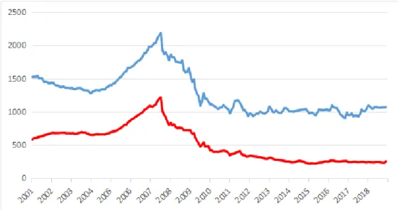
Fact 2: Financial bubbles have been popping and bursting here and there, and their macroeconomic consequences are dramatic. Japan experienced a lost decade since the burst of a stock and housing market bubble in the 90’s. The bust of the mortgage-backed securities (MBS) bubble in the US in 2008 led to a worldwide collapse.

Figure 2: Outsanding Commercial Paper in the US in Trillions of Dollars, Total (blue) and Asset-Backed (red), from 2001 to 2018. Source: FRED

Fact 3: Income and wealth inequality have sky-rocketed in developed economies since the 70’s. By providing a huge volume of new data, Piketty (2014), among others, brought awareness of those ’internal imbalances’.

Figure 3: Post-tax income shares of the top 1% (blue) vs the bottom 99 % (red) in the US from 1970 to 2009. Source: WID

(14)

Facts 1 and 2 are crucial to understand the Great Recession of 2008 in the US. Indeed, prominent authors such as Summers(2013) and Krugman (2013) have advanced the idea that the burst of a financial bubble was "the" shock that initiated the crisis. Furthermore, ultra-low real interest rates prevented the major central banks to respond adequately. At first glance, fact 3 doesn’t seem to belong to this list: it doesn’t appear especially relevant for a macro-economist interested in business cycles and financial crisis. However, since 2008, several economists2_{have informally concluded that} the huge inequality shock observed in developed economics was an important driver behind facts 1 and 2.

This "conventional" story is usually framed as follows: in the data, we observe that wealthy households have higher savings rates than poor households. Thus, a higher concentration at the top of the income distribution (fact 1) should raise the aggregate demand for assets. If the aggregate asset supply isn’t affected by this inequality shock, the equilibrium interest rate must fall in order to clear the financial markets (fact 2). As the interest rate turns very low, agents have incentives to invest in, or create, asset bubbles (fact 3). According to this logic, fact 3 implies fact 1, and fact 1 implies fact 2: the inequality shock promotes the emergence of financial bubbles.

The implication between facts 1 and 2 is well-known since the seminal work ofSamuelson(1958) andTirole(1985). Both papers have proven that "dynamic inefficiency" – i.e R < g where R is the interest rate and g the growth rate of output, both measured in steady state – is a necessary and sufficient condition for the existence of rational asset bubbles. Intuitively, if the economy cannot produce enough assets, too much savings are chasing too few stores of value: there’s a shortage of assets (Caballero,2006), and financial bubbles become attractive to investors, even through they’re inherently unproductive. But fact 3 has been barely included in the literature on rational bubbles: this paper attempts to fill this gap. Clearly, if one accepts the idea that asset bubbles can be major drivers of business cycles, then it is crucial to better understand how to prevent those bubbles in the first place, that is, to understand which circumstances promote the emergence of asset bubbles. Although very intuitive, the "conventional" story makes several assumptions, more or less im-plicitly. In this paper, I relax two of those assumptions: rather than being perfect substitutes to each others, some assets are more liquid than others – I’ll use the following definition of liquidity: liquid assets can be traded by all agents whereas illiquid assets cannot be traded by some agents; and wealthier households hold a much higher fraction of illiquid assets in their portfolio 3_{. With}

2_{Examples include:} _Stiglitz₍₂₀₀₉_),_Bardhan₍₂₀₀₉_{) or}_{Fitoussi and Saraceno}₍₂₀₁₀_).

3_{Recent studies find empirical support for the hypothesis that the equity premium is, at least partially, a}

(15)

regard to the conventional story, this adds a composition effect to inequality shocks. Indeed, an inequality shock now affects both the average savings rate but also the average desired fraction of liquid assets in agents’ portfolio. Taking this composition effect into account turns the inequality-interest rate-asset bubbles nexus upside down: if asset bubbles are liquid, a high concentration of income at the top of the distribution doesn’t promote the emergence of financial bubbles, but a low concentration does.

The model I’ll present has heterogeneous agents and imperfect financial markets that limit arbitrage between liquid vs illiquid assets. When financial frictions are non-binding, financial markets are functional, i.e arbitrage-free. As liquid and illiquid assets are perfect substitutes to each others, an inequality shock only has a level effect: by redistributing income from agents who have a low savings rate to agents who have a high savings rate, it raises asset demand, lowers the interest rate, and, if the interest rate falls enough, it makes rational bubbles possible. Thus, the model is able to reproduce the conventional story.

However, when financial frictions are binding, financial markets are dysfunctional and not arbitrage-free. Instead, liquid assets pay a liquidity premium under illiquid assets: the interest rate is lower than the rate of return on illiquid assets; this liquidity premium is the relative price of illiquid vs liquid assets. An inequality shock has dramatically different implications for the interest rate. Indeed, it redistributes income toward agents who have a higher savings rate, but also hold much less liquid assets in their portfolio. Hence, an inequality shock still raises asset demand and decreases the rate of return on illiquid assets. But, it simultaneously reduces the demand for liquid assets relative to illiquid assets, implying a fall in the liquidity premium, and therefore a higher interest rate despite a lower rate of return on illiquid assets. Consequently, the higher interest rate prevents the emergence of liquid rational bubbles; the lower rate of return on illiquid assets promotes the emergence of illiquid rational bubbles despite a higher interest rate. Thus, the model also underlines that the conventional story isn’t robust: binding financial frictions together with another layer of heterogeneity (portfolio choices) turn the results upside down.

I build a standard two-periods OLG model with competitive markets, a single consumption good, three factors of production: capital, skilled and unskilled labor, two liquid assets: bonds and bubbles, one illiquid asset: equity-capital, and two types of agents: investors and workers. Inequality are to be understood as diﬀerences in permanent income in a class society: there isn’t stock market is estimated at around 40%; and large, wealth- or income-dependent, portfolio differences are well documented.

(16)

any income risk nor social mobility. Instead, workers and investors differ at birth along three dimensions: (i) investors supply skilled labor whereas workers supply unskilled labor – skilled labor is relatively scarcer, and therefore better remunerated; (ii) investors are more patient than workers; (iii) they face different investment opportunities: workers hold liquid assets only, whereas investors can take advantage of any arbitrage opportunity between liquid and illiquid assets. Agents within one class are homogenous, there’s a fixed mass of each type.

Those assumptions are very tractable ways to capture differences in portfolio choices and savings rates that would arise in a fully-fledged model that includes (ii): idiosyncratic shocks to labor endowment as well as (iii): non-linear costs of re-balancing portfolios. Those classes should be thought of as the "99%", the workers, vs the "1%", the investors, or any other arbitrary segmentation of the population such that there are fewer investors who differ from the rest of the population because (i) they earn more, (ii) they have a higher savings rate and (iii) they have a much higher fraction of illiquid assets in their portfolio. The income distribution is calibrated by a parameter in the production function that determines how the aggregate labor income is distributed between skilled vs unskilled labor, i.e between investors vs workers. If the workers receive a high share of the aggregate labor income, I’ll say that the society is relatively equal: agents in the bottom of the distribution collectively earn a large fraction of aggregate income. An "inequality shock" is an exogenous redistribution of income from the workers to the investors – it is micro-founded by a shock to the production function that changes the optimal input mix of the firm, which starts to demand more skilled labor and less unskilled labor.

All agents face other financial frictions: they cannot short-sale the asset bubble, and their supply of bonds is limited by a borrowing constraint. In equilibrium, equity-capital is the only asset in positive net supply: all savings must be channeled to the capital market. Investors act as financial intermediaries between workers and the firm: they sell liquid bonds to the workers and accumulate illiquid equity issued by the firm. The equilibrium asset demand equals the sum of all agents’ savings; the equilibrium demand for liquid assets equals workers’ aggregate savings. Quite intuitively, a shock to the income distribution affects both: if the society becomes more unequal, asset demand rises because investors have a higher savings rate, but the demand for liquid assets shrinks because investors directly accumulate equity – they don’t use financial intermediation. As the shock doesn’t affect the equilibrium supply of assets, it simultaneously raises the rate of return on liquid assets (the interest rate) and reduces the rate of return on illiquid assets (the marginal product of capital).

(17)

If asset bubbles are liquid, a high level of inequality prevents the emergence of rational asset bubbles; if asset bubbles are illiquid, or all assets are perfect substitutes to each others, a high level of inequality promotes the emergence of rational asset bubbles. Whether the "conventional" story is right (asset bubbles arise because of rising inequality) or wrong (asset bubbles arise despite rising inequality) depends on financial markets imperfections and the type of asset bubble under consideration. With regard to the impact of an inequality shock on the size of the equilibrium asset bubble (that is, conditional on existence), we observe the same phenomenon: an inequality shock inflates already-existing financial bubbles when financial markets are functional or asset bubbles illiquid, but deflates those bubbles when financial markets are dysfunctional and asset bubbles liquid.

Of course, the way the model includes heterogeneity, inequality and financial frictions is very crude: the framework developed in this paper is too simplistic to offer a definitive conclusion about the inequality-interest rate-asset bubbles nexus. However, it allows to capture this additional effect on asset demand: total asset demand vs the demand for a particular class of asset. It is entirely conceivable, and even quite intuitive, that a higher level of inequality in the distribution of wealth or income leads to both a higher demand for assets in general and a lower demand for specific asset class (here, liquid).

One way to understand the sub-prime crisis is through the lens of the housing market (an arguably illiquid asset). Another is through the lens of the mortgage-backed securities (MBS) market (an arguably liquid asset). This model is rather coherent with the latter: as the demand for liquid assets has steadily increased over the last 30 years in the US, banks had high incentives to issue as much liquid assets as possible. To do so, they began to lend a lot in order to issue mortgage-backed liquid assets: according to this interpretation, the high housing prices pre-2008 were a by-product of the MBS bubble (as banks started to lend much more for housing-purposes, housing demand rose a lot more than the supply, hence leading to rising prices). This model doesn’t provide any explanation of how to engineer an asset bubble, but provides a narrative that questions whether asset bubbles arise because of or despite an increasing concentration of income and wealth at the top of the distribution.

Nevertheless, the predictions of the model are at odds with the data along some dimensions. In particular, if inequality is rising and ﬁnancial markets imperfect, the model predicts a higher interest rate and a lower marginal product of capital. In the data, we rather observe a more or less stable marginal product of capital, and a falling interest rate. But the model doesn’t include other

(18)

well-documented macroeconomic trends, including rising mark-ups, changes in productivity and population growths, the savings glut etc. Anyway, this paper makes a simple theoretical point: the "conventional" story is very fragile; it is perfectly conceivable that higher income and wealth inequality were a "stabilizing" force from a macroeconomic point of view.

Related literature Since Samuelson (1958) and Tirole (1985), it is well-known that as-set bubbles are possible if and only if the real interest rate is lower than the growth rate of output in steady state. More recently, Martin and Ventura (2012) and Farhi and Tirole (2012) have introduced ﬁnancial frictions in the literature on rational bubbles. This allows to disconnect the interest rate from the rate of return on other assets: asset bubbles become possible even if the marginal product of capital (the rate of return on illiquid assets) is above the growth rate of output – the relevant interest rate in the R < g condition becomes the highest rate of return the most constrained agent can reach.

I build on those papers, and in particular on Martin and Ventura (2016) who also develop an OLG model with financial frictions, heterogeneous agents and asset bubbles. They show that, if agents have linear preferences, illiquid bubbles can raise investment and output. Indeed, by providing the investors (they call them entrepreneurs) with higher collateral, illiquid asset bubbles raise the interest rate, which induces the savers to fully postpone their consumption into old-age, i.e it generates a savings glut. Although the basic structure of my model is quite similar to their, my focus is different. I don’t try to provide a theory as off why asset bubbles might be expansionary, but rather how the income distribution affects the existence condition as well as the equilibrium size of those bubbles. To do that, I introduce two types of labor associated to the two types of agents. This allows me to calibrate the income distribution and study what’s going on in the model when one makes this distribution vary – the income distribution in Martin and Ventura (2016) is very simple: young investors receive nothing and optimally decide not to consume; young workers receive the entire labor income and may decide to consume (if the interest rate is low) or to fully postpone consumption (if the interest rate is high). I also introduce liquid asset bubbles as well as differences in discount rates.

Graczyk and Phan (2018) also analyze the eﬀects of within-cohort inequality on asset bubbles using an OLG model with heterogeneous agents. In their endowment economy, all agents have the same preferences and face the same set of investment opportunities. They ﬁnd that an inequality shock promotes the emergence of asset bubbles. Indeed, as in their model, all agents receive the

(19)

same old-age endowment but different young-age endowment, poor agents want to borrow whereas wealthy agents want to save, both for a consumption-smoothing motive. This is another way of micro-founding the conventional story. In my paper, inequality interacts with heterogeneous investment opportunities and preferences. If financial frictions are non-binding, I recover their result (although through a completely different mechanism); but, if financial frictions are binding, an inequality shock prevents the emergence of liquid asset bubbles whereas it promotes the emergence of illiquid asset bubbles.

Using a three-periods OLG model with financial frictions, Raurich and Seegmuller(2017) show that the distribution of income by age-group, i.e young, middle-age and old, is a crucial determinant of whether asset bubbles are possible or not, as well as whether they’re productive or unproduc-tive. While they focus on financial intermediation between agents of different cohorts and the a-synchronicity between investment opportunities and income along the life-cycle, I rather focus on income inequality, heterogeneous investment opportunities and financial inter-mediation within one cohort. Both approaches are complementary.

Closely related areIkeda and Phan(2015) andBengui and Phan(2018). Both papers introduce financial frictions in OLG models. They distinguish between safe and risky bubbles, and study how various structural attributes of the financial markets, such as the degree of pledge-ability, the possibility of default or limited liability, promote the existence of one type of bubbles or the other. I introduce a different set of financial frictions, inequality, and I rather distinguish between liquid and illiquid bubbles. Again, both approaches are complementary.

Finally, there’s a growing literature on secular stagnation that seeks to explain the downward trend in the interest rate over the last decades in developed economies. Examples include the three-periods OLG model of Eggertsson et al. (2017) and the Bewley-like incomplete markets’ model of Auclert and Rognlie (2018). A general conclusion of this literature is that inequality was an important, although probably not the most important, factor. But those papers typically abstract from the distinction between liquid vs illiquid assets and portfolio differences, or don’t consider the possibility of dysfunctional financial markets, which are key elements of this paper. Indeed, how the liquidity premium adjusts to inequality shocks is the driving force that generates positive co-movements between the interest rate the aggregate demand for assets in my model. Section 2 introduces the model and derives the system of equations that characterizes an equilibrium; section 3 studies how inequality affects the long run interest rate when asset bubbles

(20)

aren’t valued; section 4introduces liquid asset bubbles; section 5 introduces illiquid asset bubbles; section 6 provides results related to equilibrium determinacy, the proof of which can be found in

A.

2 Basic environment and equilibrium

The basic setup is an OLG model with a single ﬁnal good, three factors of production: capital, skilled and unskilled labor, and three assets: a real bond, equity-capital and asset bubbles. Time is discrete, t ∈ {0, 1, ....}, and the horizon inﬁnite. Agents have perfect foresight; all markets are competitive. In period 0, old agents are endowed with I−₁ >0 units of equity and H = 1 units of

bubbles.

2.1 Production

A ﬁrm uses capital, Kt, and labor – skilled, Nti, and unskilled, Ntw, to produce the ﬁnal good

according to a Cobb-Douglas technology: Yt= Ktα

�

N_tiγN_tw1−γ�1−α, α, γ ∈(0, 1) (1)

Capital takes one period to build, and it fully depreciates during the production process. In period t, the ﬁrm issues Kt+1 units of equity in order to build capital in t + 1. Firm’s factor demand

functions are: W_tiN_ti Yt = γ(1 − α), WtwNtw Yt = (1 − γ)(1 − α), QtKt Yt = α (2)

Qtis the rate of dividends on equity and Wtjis the wage rate for type-j labor, j ∈ {i, w}, respectively

equal to the marginal products of capital and type-j labor in equilibrium.

Here, a higher γ raises ﬁrm’s demand for skilled labor but decreases the demand for unskilled labor. Thus, given the labor supply, the wage rate for skilled labor increases whereas that for unskilled labor decreases, implying corresponding changes in type-j labor share in aggregate income.

2.2 Households

At the beginning of period t, a new generation of agents appears. Those agents live two periods, young and old. A generation is made up of investors and workers. Those agents diﬀer along three dimensions: (i) productivity / labor type; (ii) discount factor; (iii) investment opportunities. (i)

(21)

is a proxy for diﬀerences in inherited skills or human capital whereas (ii) and (iii) are proxies for idiosyncratic shocks to labor endowment as well as non-linear costs of adjusting asset holdings. To simplify the analysis, I focus on a class society à la Matsuyama (2000) and neglect within-class heterogeneity. Those classes should be thought of as the "99%", the workers, vs the "1%", the investors, or any other arbitrary segmentation of the population such that there are fewer investors who diﬀer from the rest of the population because (i) they earn more, (ii) they have a higher savings rate and (iii) they have a much higher fraction of illiquid assets in their portfolio. Although very simplistic, this framework is complex enough to capture and question the conventional intuition.

Each generation consists of a mass λ ∈ (0, 1) of investors and a mass 1 − λ of workers. Agents within one class are homogenous; superscript j = i will denote investors, while superscript j = w will denote workers. An agent of generation t and type j derives utility from young-age consumption, C_1tj, as well as old-age consumption, C_2+t1j ,

Utj ≡log C j

1t+ βjlog C j

2t+1, βj ∈(0, 1)

Investors are relatively more patient than workers, βi_{> β}w_{: this ﬁrst layer of heterogeneity captures}

in a simple way the fact that wealthy households save more than non-wealthy households, which is necessary to reproduce the conventional intuition.

A young agent inelastically supplies one unit of labor of type j, consumes and accumulates three types of assets: real bonds, Lj

t, issued by other young agents; bubbles, H j

t, sold by older agents;

and equity, Ij

t, issued by the ﬁrm. His per-period budget constraint is:

C_1tj + Lj_t+ BtHtj+ I j t = W

j t

Income-wise, the only diﬀerence between a young worker and a young investor is the type of labor each supplies. Under assumption 1 below, skilled labor is both more demanded and less supplied than unskilled labor: in equilibrium, young investors will earn a higher wage rate than young workers.

Assumption 1 γ > λ

The within-cohort income distribution is calibrated by two parameters: γ governs the distribution of labor income between classes; λ governs the distribution of population between classes. However, as all policy functions will be linear in income, λ won’t aﬀect the aggregate variables which will

(22)

depend on γ only. Thus, I’ll call an exogenous positive variation of skilled labor share in aggregate income, i.e in investors’ aggregate income share, d log γ > 0, an inequality shock.

In his second period of life, the retiree collects returns on his asset holdings, sells his stock of bubbles and consumes his entire income,

C_2t+1j = RtLjt + Bt+1Htj+ Qt+1Itj

Here, Rtis the real interest rate.

There are three forms of ﬁnancial frictions in this economy. First, agents cannot short-sale the asset bubble,

H_tj ≥0

Second, agents’ portfolio must satisfy a borrowing constraint, Lj_t ≥ −ρQt+1

Rt

I_tj − ρBt+1 Rt

H_tj, ρ ∈(0, 1)

The supply of bonds, −Lj

t, is bounded from above by the future discounted returns the agent is

able to pledge. Although agents cannot borrow using the asset bubble because they cannot commit to repay, holding asset bubbles allow them to pledge higher returns (although not the full returns, because of the commitment problem). Here, Lj

t can be thought oﬀ as a form of backed credit

whereas Hj

t is a form of un-backed credit.

Third, the equity market is segmented,

I_tw = 0 (3)

Workers cannot hold any equity. Thus, the entire capital stock of the economy belongs to the investors, who act as ﬁnancial intermediaries between workers and the ﬁrm in equilibrium.

This last assumption is too simplistic since middle-class agents own stocks and housing. But richer agents invest a much larger fraction of their wealth in illiquid, high-returns, assets. Fur-thermore, those agents own and manage the largest banks and ﬁrms, which issue liquid assets and accumulate illiquid assets.

As both types of agents have free access to the markets for bubbles and bonds, I’ll refer to those assets as liquid, or liquidity – respectively bubbly and "fundamental"; a contrario, as the worker cannot buy any equity, the capital market is illiquid.

(23)

Lemma 1 In equilibrium, the following non-arbitrage conditions must be satisfied:

Qt+1 ≥ Rt, Bt=

Bt+1

Rt

and Bt≥0 (4)

Because all agents can trade in liquid assets, bubbles and bonds must oﬀer the same rate of return in equilibrium (Bt= Bt+1= 0 if bubbles aren’t traded). But the various ﬁnancial frictions place a

limit to arbitrage between liquid and illiquid assets4_{. Consequently, the equity must be at least as} attractive as liquid assets to investors, Qt+1 ≥ Rt, but it can oﬀer higher returns in equilibrium.

Thanks to logarithmic preferences, both types save a constant fraction of their labor income,

I_tj+ Lj_t+ BtHtj = sjWj (5)

Where sj _≡ βj

1 + βj

Since workers don’t have access to the equity market, (3), and the two types of liquid assets oﬀer the same rate of return, (4), workers’ portfolio is indeterminate in partial equilibrium.

Investors, however, are capable of taking advantage of arbitrage opportunities between liquid and illiquid assets. If both types of assets oﬀer the same rate of return, Qt+1 = Rt, investors’

portfolio is also indeterminate in partial equilibrium. But, if liquid assets pay a liquidity premium under illiquid assets, Qt+1 > Rt, there’s an arbitrage opportunity: investors can borrow from other

households at a low interest rate, lend all raised funds to the ﬁrm at a higher rate of return, and hence make free money out of it. As they implement this strategy, they issue liquid assets until they hit the borrowing constraint, and invest all funds on the equity market. Thus, if Qt+1 > Rt,

investors’ liquid asset demand functions can be written as:

Li_t= − ¯Lt, Hti = 0 (6) Where ¯Lt≡ ρQt+1 Rt 1 − ρQt+1 Rt siW_ti

Given (6), we can use (5) to determine the equity demand function.

Here, ¯Lt is the maximal supply of liquid assets consistent with the borrowing constraint.

Through the maximal leverage (debt-savings ratio), i.e ρ

Qt+1 Rt

1−ρQt+1

Rt

, it is endogenously determined by

4_{Short-sales and borrowing constraints bound the supply of liquid assets from above: investors cannot issue as}

much liquidity as they wish to; market segmentation bounds the demand from below: workers buy liquid assets even if they are dominated by illiquid assets.

(24)

the interest rate spread between liquid and illiquid assets, Qt+1

Rt . A higher spread allows investors

to pledge higher discounted returns, and therefore to issue more debt and invest more.

It is perhaps surprising that "poor" agents lend to "wealthy" agents. But both types save because they anticipate retirement. Here, agents aren’t temporarily poor or wealthy, they re-main so permanently. Thus, the income distribution doesn’t affect incentives to save/borrow for a consumption-smoothing motive: inequality in this model refers to differences in permanent income, rather than temporary fluctuations around a given average. But wealthy agents have the oppor-tunity to borrow at a low cost to invest in high-return assets: they act as financial intermediaries between the workers and the firm.

The income distribution, γ, affects both the level of asset demand – agents have different savings rate – as well as its composition – agents make different portfolio choices. In partial equilibrium, a higher level of inequality, i.e d log γ > 0, tends to affect both the level and composition of asset demand. Indeed, on the one hand, the typical investor has a higher savings rate than the typical worker: the aggregate demand for assets rises; one the other hand, the typical worker holds only liquid assets whereas the typical investor wants to sell liquid assets: the demand for liquid assets falls.

2.3 Equilibrium

In the rest of the paper, bt≡ _(1−α)YBt _t will denote the bubble-labor income ratio.

Market for bubbles In equilibrium, young agents must buy the entire stock of bubbly asset sold by older agents: λHi

t+ (1 − λ)Htw = 1; and a standard non-arbitrage condition must be

satisﬁed: bt+1 = Rt( Kt+1 Kt )−α_b t (7)

I made use of (1) and (2) to re-write (4) in terms of bubble-labor income ratio and capital stock.

Labor markets Equalizing labor demand, (2), to labor supply for each type,

W_ti= γ λ(1 − α)Yt, W w t = 1 − γ 1 − λ(1 − α)

Under assumption1, an investor receives a higher labor income than a worker. Note also that the distribution of labor income between classes is ﬁxed: on aggregate, investors receive a share γ of

(25)

the aggregate labor income. Since all policy functions are linear in income, there’s a representative worker as well as a representative investor. Given the income distribution between classes, λ determines the income level of each individual, which is neutral on aggregate.

Equity market From (2), the rate of dividends equals the marginal product of capital. Using (1) to re-write in terms of capital stock:

Qt+1 = αK_t+1α−1 (8)

Firm’s supply of equity only depends on the rate of dividends: it isn’t aﬀected by asset bubbles or inequality. To compute the economy’s stock of capital, we can use the liquidity market clearing condition, λLi

t + (1 − λ)Lwt = 0, as well as the savings function, (5), to determine investors’

equilibrium equity demand and impose market clearing, It= Kt+1:

Kt+1= � siγ+ sw(1 − γ) − bt � (1 − α)Kα t (9) And in period 0, K0 = It−1.

From an aggregate point of view, capital is the only asset in positive net supply: in general equilibrium, investors’ equity demand equals the aggregate asset demand, which is the sum of all agents’ savings (including old agents dis-savings when bubbles are valued). Indeed, investors collectively issue just enough liquid assets to meet workers’ demand, −λLi

t= (1 − λ)Lwt, and use

those borrowed funds together with their own savings to accumulate equity.

Thanks to logarithmic preferences, the aggregate asset demand is fully inelastic with respect to the interest rate. The aggregate savings rate: st≡(siγ+ sw(1 − γ) − bt)(1 − α), is aﬀected both

by the distribution of income between classes (γ) and generations (α, b). Indeed, young investors have a lower marginal propensity to consume (MPC) than young workers, who them-selves have a lower MPC than old households. Hence, any redistribution of income between those agents aﬀects the aggregate asset demand and hence the economy’s stock of capital: I’ll speak of the level eﬀect.

dlog Kt+1 = (si_{− s}w_)γ si_γ_{+ s}w_{(1 − γ) − b} t dlog γ − bt si_γ_{+ s}w_{(1 − γ) − b} t dlog bt

In particular, as si _{> s}w_{, an inequality shock has a positive level eﬀect: it increases asset demand}

(26)

asset buyers (young agents) to asset sellers (old agents), has a negative level eﬀect: it decreases asset demand and the equilibrium stock of capital.

Debt market Since the economy is closed, liquidity is in zero net supply: λLi_t+ (1 − λ)Lw_t = 0. As workers’ demand for liquid assets is fully inelastic, investors’ supply must adjust in general equilibrium to ensure that all savings are channeled to the capital market. To determine the interest rate consistent with this condition, it is necessary to distinguish between the two cases depicted in lemma1. Let ¯Lc_t ≡ _1−ρρ si(1 − α)K_tαbe the maximal supply of liquidity of an individual investor when the liquidity premium is nil, i.e Qt+1= Rt.

As long as workers’ aggregate demand for liquid assets remains limited, that is, as long as: (1 − λ)Lw

t ≤ λ ¯Ltc, ﬁnancial markets are functional, meaning arbitrage-free. The supply of liquidity

by the investors is inﬁnitely elastic: Qt+1 = Rt, and ﬁnancial constraints are irrelevant. I’ll refer

to this regime as to either "functional ﬁnancial markets", or the "high-liquidity", h-, regime. But, as the demand for liquidity rises relative to the supply, liquidity becomes scarce: (1 − λ)Lw

t > λ ¯Lct,

and financial markets turn dysfunctional, not arbitrage-free. Indeed, if all assets offer the same rate of return, investors aren’t able to issue enough debt to meet the demand. Instead, to clear the financial markets, the interest rate must fall under the rental rate of capital: Qt+1 > Rt,

until: (1 − λ)Lw

t = λ ¯Lt. This liquidity premium, Q_Rt+1_t > 1, raises investors’ maximal leverage ,

allowing them to borrow more. I’ll refer to this as to either "dysfunctional ﬁnancial markets", or the "low-liquidity", l-, regime.

To summarize, we can write the liquidity market clearing condition as: Rt= min � ρ� siγ+ sw(1 − γ) − bt� sw_{(1 − γ) − b} t ,1 � Qt+1 (10)

Given the rate of return on equity, the liquidity market clearing condition determines the interest rate spread. When liquidity is abundant, the economy is in regime h: the interest rate spread is nil, and the interest rate is determined by the aggregate asset supply and demand. However, when liquidity is scarce, the economy is in regime l: through the liquidity premium, the interest rate is also shaped by the supply and demand for liquid assets. Liquidity is scarce when the supply of liquid assets – the pledged fraction of equity-investment, ρ�

siγ+ sw(1 − γ) − bt�(1 − α), is lower

than the demand for liquid assets, (sw_{(1 − γ) − b}

t)(1 − α), both measured as shares of output; this

condition is equivalent to (1 − λ)Lw

(27)

Those two regimes have drastically different implications for the interest rate, at least given the rate of return on equity. Indeed, in regime l, any shock that impacts the supply or demand for liquid assets affects the interest rate because it changes the relative price of liquid vs illiquid assets, i.e it affects the liquidity premium, even if the shock leaves the aggregate asset supply and demand constant. This is the composition effect. In regime h, this composition effect vanishes: all assets are perfect substitutes to each other.

Through the composition eﬀect, the liquidity premium in regime l is decreasing as the asset bubble grows bigger and also as the income distribution gets more unequal.

dlogQt+1 Rt = − � (si_{− s}w_)γ si_γ_{+ s}w_{(1 − γ) − b} t + swγ sw_{(1 − γ) − b} t � dlog γ − � _b t sw_{(1 − γ) − b} t − bt si_γ_{+ s}w_{(1 − γ) − b} t � dlog bt

Indeed, a lower workers’ share in income reduces workers’ demand for liquid assets, and it simultaneously raises the supply of liquid assets because investors accumulate more equity and therefore have higher returns to pledge. Through similar mechanisms, a bigger asset bubble reduces both the supply and demand for liquid assets, but the latter is relatively more aﬀected – the second term between brackets is clearly positive.

Equilibrium Given K0 > 0, an equilibrium is a sequence {bt, Qt+1, Kt+1, Rt} such that

(7), (8), (9) and (10) are satisﬁed, Kt+1≥0 and bt≥0, for all t ≥ 0.

3 Income distribution and the interest rate

Let’s ﬁrst assume that bubbles aren’t valued in the long run. There’s always a unique "funda-mental" steady state:

b= 0 R∗ = min � ρ� siγ+ sw(1 − γ)� sw_{(1 − γ)} ,1 � Q∗ Q∗ ₌ α (si_γ_{+ s}w_{(1 − γ)) (1 − α)} K∗ ₌ � siγ+ sw(1 − γ)� 1 1−α _{(1 − α)}_1−α1

(28)

Investors act as financial intermediaries: they borrow from the workers in order to lend to the firm. Because agents have logarithmic preferences and prices are flexible 5_{, financial frictions are} irrelevant to the steady state stock of capital and output: it is "as if" all agents had access to the equity market. However, the distribution of income between classes is important if agents have heterogeneous preferences. Indeed, as workers are less patient than investors, an inequality shock that redistributes income from the workers to the investors, captured by a higher γ, raises the aggregate savings rate and the long run stock of capital.

Proposition 1 Assume that b = 0. In steady state:

1. Financial markets are dysfunctional if and only if γ < γc_.

2. If financial markets are functional, an inequality shock reduces the interest rate as well as the marginal product of capital: dlog R_d_{log γ}∗ = dlog Q∗

dlog γ <0.

3. If financial markets are dysfunctional, an inequality shock increases the interest rate but re-duces the marginal product of capital: d_dlog Q_{log γ}∗ <0 < d_dlog R_{log γ}∗.

Where γc _≡ sw(1−ρ)

sw_(1−ρ)+si_ρ ∈(0, 1).

But, as proposition1 illustrates, financial frictions greatly matter for the inequality - interest rate nexus. While the conventional intuition – that a redistribution from agents whose savings rate is low to agents whose savings rate is high lowers the interest rate – is verified when financial markets are functional, it is turned upside down when financial markets are dysfunctional. Instead, a redistribution of this kind leads to both a higher interest rate and a lower marginal product of capital in the long run. In this model, inequality affects asset demand through both a level effect – on which the conventional intuition is based – but also a composition effect: the demand for liquid assets may well rise while the aggregate demand for assets falls.

The intuition goes as follows. Although the typical worker cannot directly accumulate capital, investors act as ﬁnancial intermediaries and allocate both their and workers’ savings on the capital market. If ﬁnancial markets are functional, i.e if (1 − λ)Lw _{≤ λ ¯}_Lc_{, liquidity isn’t particularly}

scarce: investors’ supply is inﬁnitely elastic. Hence, the interest rate is the price of all assets, and it is shaped by the aggregate asset supply and demand: there isn’t any composition eﬀect. A redistribution of income from the workers to the investors raises the aggregate savings rate, i.e it

5_{Implying: (i) agents’ savings rates don’t depend on the interest rate; (ii) the interest rate adjusts to clear the}

(29)

raises asset demand. As it leaves firm’s supply unaffected, the interest rate must fall to clear the financial markets: dlog R∗_{= d log Q}∗ dlog Q∗ _{= −} (s i_{− s}w_)γ si_γ_{+ s}w_{(1 − γ)}dlog γ

However, if the ﬁnancial markets are dysfunctional, liquidity is scarce and pays a liquidity premium under the rate of dividends: without this liquidity premium, investors aren’t able to pledge enough returns to meet the demand for liquid assets by the workers. Any transfer from the workers to the investors simultaneously raises the aggregate asset demand – the aggregate savings rate increases, raises the supply of liquid assets – that is proportional to investors’ pledged returns – and decreases the demand for liquid assets – workers’ income, and hence liquidity demand, shrinks. This leads to a lower marginal product of capital, a lower liquidity premium and a higher interest rate:

dlog R∗ ₌ � (si_{− s}w_)γ si_γ_{+ s}w_{(1 − γ)} + 1 � dlog γ + d log Q∗ dlog Q∗ = − (si− sw)γ si_γ_{+ s}w_{(1 − γ)}dlog γ

Crucially, whether financial markets are functional or dysfunctional is also determined by the income distribution. Given financial markets frictions, that is, given ρ, more unequal societies, that is, with a higher γ, are less likely to have dysfunctional financial markets. Indeed, if those agents who cannot access all financial markets receive a low aggregate income share, the demand for liquid assets will be low. Thus, even through the supply of liquid assets is severely limited, those financial frictions are irrelevant.

4 Asset bubbles, the interest rate and inequality

Given the supply, a strong demand for a speciﬁc class of assets puts upward pressures on its price. In particular, if there’s either a very high demand for liquid assets – l-regime – or a very high demand for assets in general – h-regime, the rate of return on those assets falls below the growth rate of output. To remedy this dynamic ineﬃciency, private agents have one great tool: asset bubbles. If they succeed in coordinating their expectations 6_{, they can create rational asset}

6_{This paper, as well as virtually the entire literature on rational asset bubbles, doesn’t provide any explanation}

(30)

bubbles. Those are assets that don’t bring any dividends nor utility, i.e they aren’t productive, but may nevertheless be valued as a way to store wealth. Even if they are in zero net supply on aggregate (old households sell to young households), they improve consumption-smoothing by redistributing income between cohorts, which reduces the aggregate asset demand.

b= max � bl≡ sw(1 − γ) − ρ α 1 − α, bh≡ siγ+ sw(1 − γ) − α 1 − α � , b >0 Rb= 1 Q= min � Ql≡ α si_{γ(1 − α) + ρα}R b_{, Q}h _{≡ R}b� k= min � kl≡�siγ(1 − α) + ρα� 1 1−α _{, k}h _≡_(α)_1−α1 �

As there’s always a fundamental steady state, if a bubbly steady state also exists, the economy has two steady states. Those aren’t necessarily in the same regime. Two types of bubbly steady states can arise, although they don’t co-exist. In one case, financial markets are functional, all agents value the bubbles. This is the old fashion dynamic inefficiency of e.g Tirole(1985), which is symptomatic of a lack of assets in general; in the other, financial markets are dysfunctional, the workers value the bubbles whereas the investors don’t. This is the "new" form of dynamic inefficiency introduced by Martin and Ventura (2012), which is symptomatic of a lack of liquid assets (or a particular class of assets, more generally).

A bubbly steady state of type j ∈ {l, h} exists under two conditions: ﬁrst, the "fundamental" interest rate must be lower than the growth rate of output, that is, either R∗

< min{1, Q∗

} or R∗ _{= Q}∗

< 1; second, the "bubbly" economy needs to be in regime j, that is, either Rb _{< Q}b _or

Rb = Qb. Both conditions can be expressed in terms of parameter γ that calibrates the income distribution.

Proposition 2 1. There’s a bubbly steady state with functional financial markets if and only if γ > max{γh_{, γ}c−b_{}. An inequality shock doesn’t affect the interest rate nor the marginal}

product of capital, but the bubble grows bigger: dlog R_{dlog γ}b = dlog Q_{dlog γ}h = 0 < d_dlog b_{log γ}h.

2. There’s a bubbly steady state with dysfunctional financial markets if and only if γ < min{γl_{, γ}c−b_{}. An inequality shock doesn’t affect the interest rate, but it reduces the marginal}

product of capital and the asset bubble: d_dlog R_{log γ}b = 0 > d_{dlog γ}log Ql,d_{dlog γ}log bl. Where γh _≡ 1−αα −sw si−sw , γc−b≡ 1−ρ si _1−αα , and γl≡1 − ρ sw_1−αα .

(31)

As proposition (2) illustrates, the way inequality affects asset bubbles is conditional on whether financial markets are functional or not. Rational asset bubbles are possible when the economy suffers from a strong lack of assets, implying a form of dynamic inefficiency. Those bubbles reduce asset demand until the interest rate is equalized to the growth rate of the economy. Thus, a lower "bubble-less" interest rate implies a larger asset bubble in steady state. But, as discussed in the previous section, the correlation between the interest rate and inequality, and therefore asset bubbles and inequality, depends on the regime the economy is in.

There’s a bubbly steady state with functional ﬁnancial markets when the workers receive a small share of output, γ > max{γh_{, γ}c−b_{}. In regime h, the liquidity premium is nil: the asset}

bubble of type h equalizes both the interest rate and the marginal product of capital to the growth rate of output. It occurs in economies that suﬀer from a lack of assets in general: investors receive a large share of output such that (i) the rental rate of capital is lower than the growth rate of the economy, γ > γh_{; (ii) the liquidity premium is nil when there’s a bubble, γ > γ}c−b_{. Both conditions}

are equivalent to a lower bound on the asset price bubble: (i) it must be traded at a positive price; (ii) the price must be high enough to equalize the rate of return on liquid vs illiquid assets.

This type of bubble is valued by all agents and completely determines the stock of capital as a function of the capital share and the growth rate of output. Thus, it "isolates" the stock of capital from any ﬂuctuations in the distribution of income that are "absorbed" by the asset bubble. In particular, very unequal societies are characterized by a high fundamental savings rate, a low fundamental marginal product of capital and hence a large asset bubble.

dlog Rb = 0 dlog Qh= 0 dlog bh = (s i_{− s}w_)γ si_γ_{+ s}w_{(1 − γ) −} α 1−α dlog γ

A contrario, there’s a bubbly steady state with dysfunctional ﬁnancial markets when the workers receive a large share of output, γ < min{γl_{, γ}c−b_{}. In this other regime, the asset bubble equalizes}

the interest rate to the growth rate of output, but it remains below the marginal product of capital. A bubble of type l is possible in economies that suﬀer from a lack of liquid assets: the investors receive a small share of output such that (i) the interest rate is lower than the growth rate of the economy, γ < γl_{; (ii) the liquidity premium remains positive when there’s a bubble, γ < γ}c−b_.

(32)

at a positive price; but the second is an upper bound: (ii) the price must be low enough such that it doesn’t equalize the rate of return on liquid vs illiquid assets.

This type of bubble is valued by the workers only. As workers’ share decreases, they demand less liquid assets which deflates the steady state bubble. But this bubble affects the interest rate through two channels: the rental rate of capital and the liquidity premium. Thus, this bubble doesn’t fully "isolate" the stock of capital from fluctuations in the income distribution. Rather, as workers’ share in income falls, there’s a simultaneous adjustment in both the liquidity premium, that increases, and the rental rate of capital, that decreases:

dlog Rb= 0 dlog Ql= − s i_γ_{(1 − α)} si_{γ(1 − α) + ρα}dlog γ dlog bl= − s w_γ sw_{(1 − γ) − ρ} α 1−α dlog γ

Note that, while a bubble of type h can emerge even if the fundamental steady state is of type l, a bubble of type l is possible only if the fundamental steady state is of type l: min{γl_{, γ}c−b_{} < γ}c_.

Indeed, as an asset bubble decreases the liquidity premium, the "fundamental" liquidity premium must be large for a bubbly steady state of type l to exist.

The correlation between asset bubbles and inequality is turned upside down when ﬁnancial markets are dysfunctional. This is quite natural given the results in the previous section: a rational bubble exists if and only if the interest rate is lower than the growth rate of output, and it grows just large enough to equalize R to g (= 1 here). Since the correlation between the level of inequality and the interest rate changes of sign when ﬁnancial markets become dysfunctional, the same change is observed when we consider the correlation between the level inequality and asset bubbles.

In this section, I implicitly considered that asset bubbles are liquid. However, if asset bubbles are illiquid, we recover the conventional story: an inequality shock promotes the emergence of assets bubble, but despite a higher interest rate.

5 Illiquid asset bubble

Until now, the asset bubble was treated as a liquid asset similar to debt. In this extension, asset bubbles are illiquid:

(33)

This condition replaces the other no-short-sales constraint: only investors can hold the bubbly asset. This is the only modiﬁcation with respect to the basic model. As now the marginal asset bubble holder is an investor, condition (4) is replaced by:

Qt+1 ≥ Rt, Bt=

Bt+1

Qt+1

, Bt≥0

Riding the bubble must provide the same rate of return as holding the equity.

Savings are still given by (5) for both types; (3) and (11) allow us to determine workers’ portfolio. If Qt+1 = Rt, investors’ portfolio is fully indeterminate in partial equilibrium. However,

if Qt+1> Rt, investors’ liquid asset demand functions can be written as:

Li_t+ BtHti= − ρQt+1 Rt 1 − ρQt+1 Rt siW_ti, H_ti ≥0

Given (6), this equation determines investors’ equity demand.

As on aggregate, agents still have the same savings rate, and ﬁrm’s program hasn’t changed, (8) and (9) remain valid. But (7) is replaced by:

b_t+1= Q_t+1(Kt+1 Kt

)−α_b

t (12)

And the liquidity market clearing condition, (10), is replaced by: Rt= min � ρ� siγ+ sw(1 − γ)� sw_{(1 − γ)} ,1 � Q_t+1 (13)

Asset bubbles don’t aﬀect the liquidity premium. Indeed, they don’t lower the demand for liquid assets by the workers: bubbles aren’t liquid, and therefore workers’ demand is nil; and they don’t decrease the supply by the investors: the lower pledged returns on equity investment are fully compensated by the higher pledged returns on riding the bubble.

Given K0 > 0, an equilibrium is a sequence {bt, Qt+1, Kt+1, Rt} such that (12), (8), (9) and

(13) are satisﬁed, Kt+1≥0 and bt≥0, for all t ≥ 0.

Of course, this modification doesn’t affect the fundamental steady state, which is similar to that of section 3. But the bubbly steady states differ. Indeed, there’s a unique bubbly steady state, which has the same bubble and capital stock as that of type h, section 4, but exists under the condition: γ > γh_{, i.e the usual dynamic inefficiency condition: Q}∗

(34)

liquidity premium: Rb = min � ρ� siγ+ sw(1 − γ)� sw_{(1 − γ)} ,1 � Qb

The dynamic of capital and asset prices are also similar to that of regime h, section 4.

Thus, illiquid asset bubbles satisfy the conventional intuition. There’s however, an important addendum when ﬁnancial markets are dysfunctional, i.e γ < γc_{: an inequality shock favors the}

emergence of ﬁnancial bubbles despite a higher interest rate. Indeed, the existence of illiquid bubbles is conditional on the rate of return on illiquid assets, which doesn’t equal the interest rate. If ﬁnancial markets are dysfunctional, an inequality shock lowers the rate of return on illiquid assets but raises that on liquid assets.

6 Dynamic and stability

The entire dynamic can be described by a 2-dimensional system with one backward-looking variable, the stock of capital, and one forward-looking, the asset price bubble:

Kt+1 = �� siγ + sw(1 − γ) − bt � (1 − α)�K_tα bt+1 =        ρα ρα+(bl−bt)(1−α) if bt< b l₊ ρ 1−ρ(b l_{− b}h₎ α α+(bh−bt)(1−α) otherwise

Given {bt}, the dynamic of the stock of capital is stable: there are equilibria as long as the asset price

bubble doesn’t explode as a share of output. The analysis of the diﬀerence equation corresponding to the asset bubble is relegated to appendixA.

Proposition 3 1. If the fundamental steady state doesn’t co-exist with a bubbly steady state, there’s a unique equilibrium: bt= 0 for all t ≥ 0.

2. If the fundamental steady state co-exists with a bubbly steady state of type j ∈ {l, h},

i. There’s a continuum of equilibria, indexed by b0 ∈ [0, bj), that converges to the

funda-mental steady state;

ii. As well as a unique equilibrium that converges to the bubbly steady state: bt= bj for all

t ≥0.

The fundamental steady state is globally determinate if and only if it is unique; if it co-exists with a bubbly steady state, it is globally indeterminate but the bubbly steady state is globally

(35)

determinate. The presence of two distinct regimes doesn’t change this conclusion, which is usual in the literature, and traces back to Tirole(1985).

7 Conclusion

I have provided a simple, analytical, model to study how inequality promotes or prevents the emergence of (rational) financial bubbles. An inequality shock promotes the emergence of financial bubbles if and only if financial markets aren’t too imperfect, or the bubble is illiquid.

This model is, of course, way too simplistic to offer a definitive conclusion on this matter. But it underlines the very importance of financial frictions to understand how inequality shapes the rates of return on particular asset classes and therefore promotes or prevents the emergence of asset bubbles of particular types.

A Bubbly dynamic

The dynamic of the bubble-labor income ratio is described by the following non-linear equation:

bt+1=        ρα ρα+(bl−bt)(1−α) if bt< b l₊ ρ 1−ρ(bl− bh) α α+(bh₋_b t)(1−α) otherwise

In a given regime j ∈ {l, h}, the dynamic is unstable: the bubble explodes as a share of output, i.e limt→∞bt → ∞, if bt > bj; it implodes, limt→∞bt = 0, if bt < bj; and it has a unique steady

state, bt= bj. A path that leads to an explosion cannot be part of an equilibrium because it would

violate either the bubble market clearing condition, or young agents’ budget constraint. A path that leads to an implosion converges to the fundamental steady state.

It is useful to distinguish three cases: (i) there isn’t any bubbly steady state; (ii) there’s a bubbly steady state of type l; (iii) there’s a bubbly steady state of type h. Remember that there’s always a unique fundamental steady state.

(i) There isn’t any bubbly steady state if and only if max{bl_{, b}h_{} < 0. Consequently, if b} 0 >0,

then b0 >max{bl, bh}: all path such that bt>0 lead to an explosion. Hence, there’s a unique

equilibrium, and it is bubble-less: bt= 0 for all t ≥ 0.

(ii) There’s a bubbly steady state of type l if and only if bl _>_{max{0, b}h_{}. As b}l₊ ρ

(36)

bl> bh, a path that starts in, or switches to, the h-regime leads to an explosion: this rules out all path such that b0 > bl. Furthermore, since bl+_1−ρρ (bl− bh) > 0 is equivalent to γ < γc,

the fundamental steady state is of type l. Hence, there’s a unique path that converges to the bubbly steady state, bt= blfor all t ≥ 0; and a continuum of paths, b0∈[0, bl), that converge

to the fundamental steady state.

(iii) There’s a bubbly steady state of type h if and only if bh _> _{max{0, b}l_{}. Here, we have:}

bl+_1−ρρ (bl− bh) < bl< bh. There are two sub-possibilities. (a) The fundamental steady state is of type h, that is, γ > γc_{. As b}l₊ ρ

1−ρ(bl− bh) < 0, the economy is always in the h-regime.

All paths such that b0 ∈[0, bh) lead to an implosion; all paths such that b0 > bh lead to an

explosion; and there’s a unique path such that bt = bj for all t ≥ 0. (b) The fundamental

steady state is in regime l, that is, γ < γc_{. Again, if b}

t > bh, the economy starts in the

h-regime, remains there, and the bubble explodes. If bt < bl+ _1−ρρ (bl − bh), the economy

starts in the l-regime, remains there, and the bubble implodes. If bt∈(bl+ _1−ρρ (bl− bh), bh),

the economy starts in regime h, but the bubble begins to implode; there’s a switch to the l-regime as soon as bt< bl+_1−ρρ (bl− bh), and the bubble continues to implode. Hence, again,

there’s a unique path that converges to the bubbly steady state, bt= bh for all t ≥ 0; and a