Physico-statistical modelling of the primary phase of an unprotected loss of flow

(1)

HAL Id: cea-02509188

https://hal-cea.archives-ouvertes.fr/cea-02509188

Submitted on 16 Mar 2020

HAL is a multi-disciplinary open access archive for the deposit and dissemination of sci-entific research documents, whether they are pub-lished or not. The documents may come from teaching and research institutions in France or abroad, or from public or private research centers.

L’archive ouverte pluridisciplinaire HAL, est destinée au dépôt et à la diffusion de documents scientifiques de niveau recherche, publiés ou non, émanant des établissements d’enseignement et de recherche français ou étrangers, des laboratoires publics ou privés.

Physico-statistical modelling of the primary phase of an

unprotected loss of flow

J.-B. Droin, N. Marie, F. Bertrand, E. Merle-Lucotte

To cite this version:

J.-B. Droin, N. Marie, F. Bertrand, E. Merle-Lucotte. Physico-statistical modelling of the primary phase of an unprotected loss of flow. NURETH 16 - The 16th International Topical Meeting on Nuclear Reactor Thermalhydraulics, Aug 2015, Chicago, United States. pp.5058-5071. �cea-02509188�

(2)

Hyatt Re ge n cy C hicago, C hicago, IL, USA, August 30 -Se pte mbe r 4, 2015

PHYSICO-STATISTICAL MODELLING OF THE PRIMARY PHASE OF AN UNPROTECTED LOSS OF FLOW

J.B. Droin1, N. Marie1, F. Bertrand1, E. Merle-Lucotte2

1

: CEA, DEN, DER, F-13108 Saint-Paul-lez-Durance, France

2

: LPSC-IN2P3-CNRS, 53 rue des Martyrs, F-38026 Grenoble Cedex, France Corresponding author: jean-baptiste.droin@cea.fr , Tel: +33 (0) 4 42 25 59 06

Abstract

The paper presents some outlines of CEA’s work on Unprotected Loss Of Flow (ULOF) using an analytical tool under development, in particular regarding boiling stabilization. It is based on analytical thermal-hydraulic models that enable very low CPU times for each simulation (compared to mechanistic tools). It will thus be used to provide large sensitivity studies on various physical parameters. In this paper, boiling stabilization possibilities are studied in the case of a low, an intermediate and a high power transient, first considering a quasi-static approach. Then, transients are simulated to highlight dynamic aspects of the problem that can’t be predicted with the quasi-static approach, such as chugging phenomenon or flow excursion transients.

1. Introduction

The current objectives of the French GenIV projects are to define a reactor design in order to improve reactor technology in terms of safety and reliability at an industrial scale. Among other concepts, the Sodium Fast Reactor (SFR) has been selected for its ability to secure the nuclear fuel resources and to manage radioactive waste. Design improvement studies of SFRs are then ongoing in France. The core design studies are carried-out by the CEA with support from AREVA and EDF. A major innovation of the new SFR French concept concerns the core which is featured by a very low (even negative) reactivity effect caused by a potential sodium voiding. This feature will more specifically have a strong impact on the primary phase of severe accidents, especially on the heating up and voiding of the sodium and on the core power evolution. It is then necessary to assess the behavior of this new core design facing severe accident transients.

Complex mechanistic codes like SIMMER and SAS enable to treat coupled thermal-hydraulic and neutronic aspects for various fast reactor severe accident transients. However, the high CPU time of each simulation of such complex codes prevents their direct use for uncertainty propagation and sensitivity studies, especially in the case of a high number of uncertain input parameters. To overcome the limitations associated to these complex mechanistic codes, the CEA follows a new approach in parallel with the use of these mechanistic tools. This approach involves some coupled analytical 0D or 1D modelling of the main physical phenomena occurring during accident transients combined with advanced statistical analysis techniques. The analytical tool presented in this paper is more specifically devoted to the Unprotected Loss Of Flow modelling.

(3)

The Unprotected Loss of Flow accident is assumed to be initiated by the primary pump rundown. Shutdown systems are supposed to fail and the transient starts at nominal power. As a consequence, the sodium flow rate is highly and progressively reduced and the core temperature increases. The sum of the reactivity feedback effects due to the core heating-up being negative, the fuel power starts to decrease. Then, depending on the flow rate decrease and on the power evolution, sodium boiling may occur. But on the contrary to cores presenting a positive void effect, with this new core design, boiling does not cause a primary power excursion. Depending on the power conditions when boiling occurs, the two-phase core flow may stabilize in the upper part of the subassemblies (SAs). However, in case of high power transient, boiling conditions may become unstable. A flow excursion transient would then lead to the downwards progression of the boiling front within the core, possibly inducing the fuel pins dry-out and the degradation of SAs. The primary phase finally ends with the first hexcan failure in the core.

After a short description of the models implemented in the analytical tool, the study of the possibilities of boiling stabilization in the upper part of SAs will be presented, firstly considering a quasi-static approach, and then by simulating the transient to take into account dynamic aspects.

2. Description of the physical models

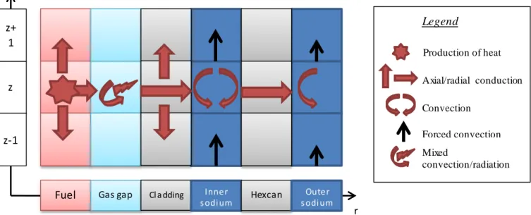
As displayed in Figure 1, the SA is modelled along a one-dimensional axial direction, by a representative pin, its surrounding coolant and its associated hexcan (as done in SAS-SFR [1]). The sodium flow is considered as unidirectional from the bottom (inlet) to the top of the SA (outlet). Variables (such as sodium density or void fraction) are space-averaged over each axial mesh.

Figure 1 – Representation of a subassembly (fuel pins region) in the analytical modelling

First, the momentum balance equation is applied to the whole SA in order to assess the inlet mass flow rate 𝑄 at each time step as explained in paragraph 2.1. Then, heating-up of sodium and structures is calculated by applying the energy balance equation to each component of the SA as described in paragraph 2.2. Outer-subassembly sodium Oz Fuel Gas gap Cladding Hexcan Inner-subassembly sodium

(4)

2.1 Flow rate decrease modelling

The momentum balance equation applied on the whole AS can be written [2]: 𝜕𝑄(𝑡)

𝜕𝑡 =

∆𝑃_𝑒𝑥𝑡(𝑡) − ∆𝑃_𝑖𝑛𝑡(𝑡) 𝑘

Equation 1

Where the following terms stand for:

- 𝑄 : inlet mass flow rate of the SA (in kg.s-1);

- ∆𝑃_𝑒𝑥𝑡 : driving (external) pressure drop (in Pa) between the two extremities of the SA (inlet and outlet) induced by the external loop (including intermediate heat exchangers and primary pumps);

- ∆𝑃_𝑖𝑛𝑡 : resistive (internal) pressure drop (in Pa) induced by a single or two-phase assuming steady-state conditions;

- 𝑘 : constant only depending on the SA’s geometry (m-1).

Calculation of the driving pressure drop (∆𝑃_𝑒𝑥𝑡)

The driving pressure drop is composed of:

- the hydrostatic pressure in the external loop (constant term corresponding to the cold sodium column weight);

- the pump pressure head (which is time-dependant). Thus, it can be expressed:

∆𝑃_𝑒𝑥𝑡(𝑡) = ∆𝑃_{𝑝𝑢𝑚𝑝}(𝑡) + ∆𝑃_{ℎ𝑦𝑑𝑟𝑜𝑠𝑡𝑎𝑡𝑖𝑐}

Equation 2

The ULOF transient is simulated by imposing a decrease of this driving pressure drop. More precisely, the pump pressure head is supposed to decrease from its nominal value down to zero following this hyperbolic law: ∆𝑃_{𝑝𝑢𝑚𝑝}(𝑡) = ∆𝑃𝑝𝑢𝑚𝑝 0 (1 + 0.91 𝑡_𝜏 1/2) 2 Equation 3

Where 𝜏_1/2 stands for the pump flow rate halving time (s) and ∆𝑃_{𝑝𝑢𝑚𝑝 0} is the initial pump pressure head (Pa). Note that the 0.91 parameter was adjusted in order to match with the flow rate decrease of CATHARE2 simulations [3].

Calculation of the resistive pressure drop (∆𝑃_𝑖𝑛𝑡)

The pressure drop along the whole SA is calculated using the following formula (assuming stead-state conditions):

(5)

Where ∆𝑃_{𝑓𝑟𝑖𝑐}, ∆𝑃_{𝑔𝑟𝑎𝑣}, ∆𝑃_𝑎𝑐𝑐 and ∆𝑃_{𝑠𝑖𝑛𝑔} respectively stand for frictional, gravitational, acceleration and singular pressure drop (in Pa).

These pressure drop terms are classically calculated in each axial mesh and then summed up on the whole SA. As far as two-phase flow is concerned, a homogeneous model approach is used: we consider an unique two-phase mixture, whose properties (such as density) are volume-averaged using the void fraction distribution. This void fraction axial distribution as the friction pressure drop is evaluated using the Lockhart-Martinelli model, which implicitly takes into account a slip between liquid and vapour phases. This model has proven to provide accurate results for sodium boiling [4]. A global disequilibrium due to radial temperature gradients in the fluid is also taken into account as recommended in [5].

Knowing the values of the resistive pressure drop (∆𝑃_𝑖𝑛𝑡(𝑡)) and of the driving pressure drop (∆𝑃_𝑒𝑥𝑡(𝑡)) at each time step, it is possible to calculate the temporal evolution of the inlet mass flow rate of the SA 𝑄(𝑡) (Equation 1). Additionally, using the conservation of the mass flow rate in the SA, it is possible to determine the sodium velocities in each axial mesh, conditioning the convection process and the cooling of the SA.

2.2 Sodium and structures heating-up and convection in the sodium flow

The energy balance equation is solved for all the SA’s elements (i.e. for the sodium, the cladding, the fuel and the hexcan), in each axial mesh of the modelling, not only to assess their heating-up, but also to calculate the quality when sodium is boiling. It is indeed necessary to determine the vapour quality distribution in order to derive the void fraction distribution from the Lockhart-Martinelli model [6].

Heat transfers that are taken into account in the energy balance equation are the followings (synthetized in Figure 2):

- 2D-conduction (axial and radial) in the fuel; - convection and radiation in the gas gap1;

- 2D-conduction (axial and radial) in the cladding; - convection in the inner-SA sodium;

- 1D-conduction (radial) in the hexcan;

- convection in the outer-SA sodium (in the inter-subassembly gap).

To quantify the convection heat transfers processes (in inner sodium as in outer sodium), the Lyon-Martinelli heat transfer correlation (referenced in [7]) is used:

𝑁𝑢 = 7 + 0.025𝑅𝑒0.8_𝑃𝑟0.8

Where 𝑁𝑢, 𝑅𝑒 and 𝑃𝑟 respectively refer to the Nusselt number, the Reynolds number and the Prandtl number.

When a single SA is considered, a constant production of heat is considered in the fuel. Note that a constant sodium inlet temperature is taken into account as a boundary condition. This assumption is reasonable at that time for modelling activities, but the core inlet temperature evolution will be considered in future applications taking into account system effects and their feed-back on core reactivity.

1

A global exchange coefficient taking into account convection and radiation is considered. Its value is currently taken from the SIMMER-III mechanistic code.

(6)

Figure 2 - Heat transfers considered in the analytical modelling (fuel pins region)

Calculating all the heat transfers occurring in the SA enables to derive space-averaged enthalpies for each component at each axial mesh. As far as two-phase flow is concerned, quality in the flow is then deduced from the sodium average enthalpy.

3. Thermal-hydraulic static, quasi-static and transient approaches

In this paragraph, some theoretical aspects of sodium boiling are firstly reported. Static stability configurations are then studied for three ULOF transients at different power levels, considering a quasi-static approach. The same transients are finally simulated with the analytical tool described in paragraph 2 to conclude about its ability to correctly reproduce the quasi-static predictions.

3.1 Definitions

The following definitions (issued from [8]) will be used in the next paragraphs.

Resistive (internal) characteristic:

The resistive characteristic is the evolution of the pressure drop along the channel (induced by a single or two-phase flow) as a function of the inlet flow rate. It is actually a succession of steady-state pressure drop measures, carried out considering constant power, outlet pressure and inlet temperature. For a sodium flow at a low pressure, the resistive characteristic is generally a “S shape” curve, as highlighted in Figure 3.

Fuel Gas gap Cl a dding Inner

s odi um Hexcan Outer s odi um z+ 1 z z-1 z r Production of heat Axial/radial conduction Convection Forced convection Mixed convection/radiation Legend

(7)

Figure 3- Typical shape of resistive (internal) characteristic in a sodium boiling channel [9] Driving (external) characteristic:

The driving characteristic is the variation in the pressure drop between the two extremities (inlet and outlet) of the SA induced by the external loop (that includes the primary pumps) as a function of the inlet flow rate of the SA.

Operating point:

An operating point is an intersection point between the resistive and the driving characteristics (for instance points A, B or C in Figure 3).

3.2 Static equilibrium criterion

An operating point is statically stable when a small disturbance on the mass flow rate does not cause a change of steady state. In other words, it is statically stable if the mass flow rate can be maintained in steady sate conditions in spite of small disturbances.

According to the Ledinegg criterion, an operating point is statically stable when the slope of the resistive characteristic curve is higher than the slope of the driving one [10]:

(𝑑∆𝑃𝑖𝑛𝑡 𝑑𝑄 ) > (

𝑑∆𝑃_𝑒𝑥𝑡 𝑑𝑄 )

Equation 4

Where ∆𝑃_𝑖𝑛𝑡 stands for the resistive (internal) pressure drop (in Pa), ∆𝑃_𝑒𝑥𝑡 for the driving pressure drop (in Pa) and Q for mass flow rate in the SA (in kg.s-1).

The operating point A in Figure 3 is statically stable according to the Ledinegg criterion. It means that it is possible to reach steady state conditions for the mass flow rate 𝑄₀.

If however this static stability criterion is not satisfied for an operating point (between point B and point D in Figure 4 for instance), a flow excursion develops from a small flow rate disturbance, also called static instability. As shown in Figure 3, the flow will decrease progressively until a new statically stable operational point is reached. Theoretically, a new stable point may be reached (point C in Figure 3), but dry-out generally occurs during the flow excursion.

(8)

Note that as far flow excursion transients are concerned, the Ledinegg criterion gives information on the initial and on the final steady states, but it provides no information about the transient between those states.

Ledinegg criterion applied to an ULOF transient leading to natural circulation:

During an Unprotected Loss Of Flow leading to natural circulation in a reactor case, the static stability criterion (Equation 4) only implies that the slope of the internal characteristics of the channels should be positive for the operating point to be statically stable:

(𝑑∆𝑃

𝑑𝑄 )_𝑖𝑛𝑡> 0

Equation 5

Indeed, at low flow rates (compared to nominal conditions), friction becomes negligible in the primary circuit. The driving characteristic is then reduced to a simple constant term (which is the cold sodium column weight) [9]. In these conditions, the driving characteristic is a horizontal line in a (Q,∆𝑃) plan.

3.3 Quasi-static approach

The quasi-static approach consists in considering the transient as a succession of steady states. In these conditions, the Ledinegg criterion enables to assess the possibilities to reach steady-state conditions. In this paragraph, this quasi-static approach is applied on a single SFR internal core SA to determine if steady-state conditions may be finally reached for:

- a low power transient (20% of the nominal power conditions2) ;

- an intermediate power transient (40% of the nominal power conditions2) ; - a high power transient (70% of the nominal power conditions2).

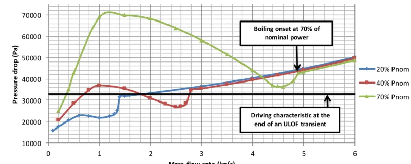
In Figure 4, resistive characteristics, calculated for each of these power levels with the analytical modelling, are presented. Pressure drops in the SA are plotted for various flow rates in steady-state conditions.

Figure 4 - Resistive characteristics of a SFR core channel calculated using the analytical tool

2

Nominal power delivered in the considered subassembly: 5.00MW. 10000 20000 30000 40000 50000 60000 70000 0 1 2 3 4 5 6 P re ss ur e dr op ( P a)

Mass flow rate (kg/s)

20% Pnom 40% Pnom 70% Pnom

Boiling onset at 70% of nominal power

Driving characteristic at the end of an ULOF transient

(9)

Description of the resistive characteristics shape:

Generally speaking, once boiling is reached (see the shape of the coloured curves on Fig. 4), if the flow rate further decreases, the pressure drop first decreases before increasing again. This phenomenon results from the balance between gravitational and frictional effects of boiling:

- when considering a quasi-static approach, boiling starts at the top of the SA for hydrostatic reasons. The voiding of the channel causes a drop of the gravitational head. In the upper part of the SA, hydraulic diameter is large (around 10cm). Frictional effects of boiling do not compensate the total pressure drop in the SA: the pressure drop globally decreases;

- if the mass flow rate is further decreased, the boiling front will enter into the pins bundle. In this part of the SA, hydraulic diameter is largely reduced (around 3mm). The significant increase of the friction pressure drop is then at the origin of the total pressure drop increase.

Conclusions regarding static stability possibilities:

The driving characteristic shown in Figure 4 corresponds to the cold sodium column weight. It represents the driving characteristic at the end of an ULOF transient, when the pressure pump head has reached zero value. At that moment, only the hydrostatic pressure in the system plays a role in the flow stability.

In these conditions (i.e. at the end of an ULOF leading to natural convection), it comes out from Figure 4 and from the Ledinegg criterion that, considering a quasi-static approach:

- under low power conditions (20% of nominal power conditions), static stability can be reached for a liquid single-phase flow (natural convection);

- under intermediate power conditions (40% of nominal power conditions), static stability can be reached for a two-phase flow (natural convection);

- under high power conditions (70% of nominal power conditions), no static stability conditions can be achieved: a flow excursion occurs during the transient.

Limits of the quasi-static approach:

A quasi-static approach however presents some limitations. Indeed, it consists in neglecting unsteady terms in the balance equations. Then, a quasi-static approach does not take into account dynamic aspects of the problem (such as thermal inertia, neutronic coupling, etc.). As far as ULOF transients are concerned, this approximation has two main consequences:

- for statically stable conditions, it is not possible to predict dynamic instabilities that may characterize the final state (such as chugging phenomenon described in [11]);

- for statically unstable conditions, it gives no information about the flow excursion transient.

The next paragraph reports transient calculations (taking into account unsteady terms in balance equations) to conclude about the analytical modelling’s ability to reproduce the quasi-static predictions and about its capability to model dynamic aspects of the problem.

3.4 Transient approach with the analytical modelling

The next transients are calculated with the analytical modelling presented in paragraph 2. ULOF transients are simulated for a single SA of the SFR internal core at constant power (no neutronic coupling is implemented yet).

(10)

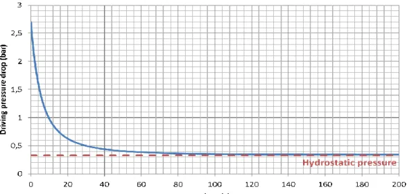
To simulate the transient, a decrease of the pump pressure head is imposed from its initial value down to zero as explained in paragraph 2.1. The halving time of the mass flow rate is 10s. The driving pressure drop then tends toward the hydrostatic pressure in the SA, as displayed in Figure 5.

Figure 5 - Driving pressure drop evolution during an ULOF transient characterized by a 10s pump halving time

This transient is simulated at three different power levels. Later on in the paper, low, intermediate and high power respectively refers to 20%, 40% and 70% of nominal power (5.00MW).

The stopping criteria for these simulations are t=500s or the first occurrence of clad melting. Note that the dry-out occurs for a specified quality of the flow (x=0.2) as demonstrated by the CASPAR calculations of the GR-19BP experiment [12].

3.4.1 Case 1: low power transient

The sodium mass flow rate evolution during the low power transient simulated with the analytical modelling is shown in Figure 6.

Figure 6 - Mass flow rate evolution during an ULOF transient (single SFR core subassembly) at constant low power (20% of its nominal value)

M as s fl ow r at e (k g. s -1 )

(11)

During this low power transient, no boiling onset is observed: the flow remains liquid. At the end of the pump pressure head decrease (i.e. when the external pressure drop has reached its hydrostatic value), the single-phase flow conditions are statically stable as predicted by the quasi-static approach and the mass flow rate naturally stabilized around 1.85 kg/s as displayed in Figure 4 (intersection of the blue resistive characteristic and the black driving one). The final steady configuration obtained with the analytical tool matches well with the quasi-static predictions at this low power case.

3.4.2 Case 2: intermediate power transient

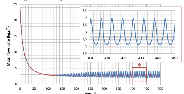
The sodium mass flow rate evolution during the intermediate power transient simulated with the analytical modelling is shown in Figure 7.

Figure 7 - Mass flow rate evolution during a ULOF transient (single SFR core subassembly) at constant intermediate power (40% of its nominal value)

From this figure, it can be seen that sodium boiling starts 127s after the pump trip. Then, stabilized boiling takes place in the SA. As predicted by the quasi-static approach, flow conditions remain statically stable in a two-phase flow regime. This is why the mass flow rate reaches its asymptotic path (red dashed line) towards its two-phase natural convection value, which is shown to be 2.8 kg/s (cf. intersection of the red resistive characteristic and the black driving one in Figure 4).

However, dynamic instabilities, which cannot be predicted with a quasi-static approach, are observed during the transient. Indeed, cyclic oscillations of the inlet mass flow rate around the steady-state value appear at the beginning of boiling until the end of the transient as seen in Figure 7. These oscillations are synchronized with the formation of vapor slugs in the channel as depicted in Figure 8. These instabilities actually correspond to a chugging phenomenon, described in [11] and observed in [3]:

- sodium boiling begins and leads to a sharp decrease of the two-phase mixture density: the internal pressure drop decreases;

- if the flow conditions are statically stable according to the Ledinegg criterion, it results in a mass flow increase in the SA, leading to a cold sodium reflooding of the two-phase zone;

- sodium reflooding leads to an increase of the gravitational component of the pressure drop; - according to the Ledinegg’s theory, it results in a decrease of the mass flow rate in the SA, and

so on... M as s fl ow r at e (k g. s -1 )

(12)

These oscillations are sustainable as long as the flow conditions are statically stable according to the Ledinegg criterion. In this intermediate power case, the boiling front never penetrates for more than 10cm inside the pins bundle (cf. Figure 8). In the part of the core where the hydraulic diameter is low, the flow remains mainly liquid. This is why the flow conditions remain statically stable.

Figure 8 - Boiling fronts evolution during an ULOF transient applied to a single SFR core subassembly at constant intermediate power (40% of its nominal value)

3.4.3 Case 3: high power transient

When simulated with the analytical modelling, this high power transient leads to the mass flow rate evolution given in Figure 9.

Figure 9 - Mass flow evolution during a ULOF transient (single SFR core subassembly) at constant high power (70% of its nominal value)

M as s fl ow r at e (k g. s -1 )

(13)

Sodium boiling starts 48s after the pump trip. As predicted by Figure 4, the two-phase flow remains stable as long as the driving pressure drop is higher than 0.36 bar. At t=62s (see Figure 5), this criterion is not satisfied anymore: a flow excursion transient occurs. The mass flow rate decreases until the theoretical high quality stable state is reached (around 𝑄 ≅ 0.5𝑘𝑔/𝑠).

Contrary to the quasi-static approach, the transient calculation gives us information about dynamic aspects of this transient. Firstly, during the stabilized boiling period (from t=48s to t=62s), the transient is characterized by dynamic instabilities corresponding to a kind of chugging. Then, the flow excursion lasts about 8s. More precisely, the mass flow rate progressively decreases until the dry-out occurrence that happens 16s after the boiling onset, causing a sharp degradation of the thermal exchange coefficient in the flow channel. As a consequence, the first clad melting is quickly observed only 3s after the first dry-out occurrence. The statically stable state, where high quality sodium boiling is theoretically possible, is not reached: degradation of the SA happens earlier.

3 Conclusion and Prospects

As part of the R&D program on GEN IV SFRs, a physico-statistical approach is currently considered to study severe accident scenarios. Within this framework, an analytical modelling devoted to the ULOF simulation is under development. It is a part of a set of tools developed by CEA to carry out uncertainty studies in parallel of the use of more complex mechanistic tools such as SIMMER and SAS-SFR. Indeed, each simulation of such complex codes requires a high CPU time, especially when neutron physics is calculated, which considerably limits the number of simulations. This prevents their direct use for uncertainty propagation and sensitivity studies, especially in the case of a high number of uncertain inputs.

In this paper, the physico-statistical tool dedicated to ULOF transients is firstly described. It is based on analytical thermal-hydraulic models and takes into account conduction in solids and convection in fluids. As far as a two-phase flow is concerned, sodium is considered as a homogeneous mixture and thermal and dynamic disequilibrium in the two-phase fluid are also taken into account. Note that only the initiating phase and the boiling transient models are presented, modelling of later steps of the accident being still under way. The analytical tool described in paragraph 2 enables low CPU-times. Simulation of transients such as described in paragraph 3.4 lasts about a minute.

For each ULOF transient (at low, intermediate and high power), the final configurations given by the analytical tool are in good agreement with the quasi-static approach predictions, regarding stabilization possibilities. In addition to that, the tool also simulates dynamic phenomena that cannot be described when considering a succession of steady states, such as chugging phenomenon or flow excursion transients. Further validation on experiments regarding these phenomena is required and is still under way.

In this paper, transients are only applied on a single SA and until the first clad melting occurrence. However, the aim of such an analytical tool is to simulate ULOF transients on the whole core and up to the end of the transient. Applications on an entire core will be performed by regrouping SAs in channels, and by computing the neutronic evolution of the fuel power using a 0D approach. The preliminary results that have already been obtained seem in good agreement with SIMMER-III results, but further analyses are still under way. In a near future, modelling of the molten cladding and fuel

(14)

relocations in the SA will be carried out (also taking into account their impacts on the global core reactivity).

4 References

[1] D. Lemasson and F. Bertrand, "Simulation with SAS-SFR of a ULOF transient on ASTRID-like core and analysis of molten clad relocation dynamics in heterogeneous subassemblies with SAS-SFR," ICAPP 2014, Charlotte, USA, 2014, April 6-9.

[2] F. Schmitt, "Contribution expérimentale et théorique à l'étude d'un type particulier d'écoulement transitoire de sodium en ébullition : la redistribution de débit", Ph.D. thesis, 1974.

[3] N. Alpy, et al. , "Phenomenological Investigation of Sodium Boiling in a SFR Core during a postulated ULOF transient with CATHARE 2 System Code: a Stabilized Boiling Case," NUTHOS-10, Okinawa, Japan, 2014, December 14-18.

[4] H. M. Kottowski, Liquid Metal THermalhydraulics, INFORUM Verlag, 1994.

[5] D. Grand, P. Mercier and J.M. Seiler, "Status of the NATREX code calculation of loss of flow transients and overpower transients in single channel geometry," 9th LMBWG, Rome, 1980, June 4-6. [6] R. W. Lockhart and R. M. Martinelli, "Proposed correlation of data for isothermal two-phase, two-component flow in pipes," Chemical Engineering Progress, vol. 45, no. 1, pp. 39-48, January 1949.

[7] F. Agosti and L. Luzzi, Heat Transfer Correlations for Liquid Metal Cooled Fast Reactors - Short Handbook, Politecnico di Milano - Department of Nuclear Engineering, 2007.

[8] J. Bouré, "Review of two-phase instability," ASME-AICHE Heat Transfert Conference, Tulsa, 1971, August 15-18.

[9] J. M. Seiler, D. Juhel and P. Dufour, "Sodium boiling stabilisation in a fast breeder reactor subassembly during an unprotected loss of flow accident," Nuclear Engineering and Design, no. 240, pp. 3329-3335, 2010.

[10] M. Ledinegg, Instability of flow during natural and forced convection, Die Warme, 1938. [11] J. M. Delhaye, Thermohydraulique des réacteurs, EDP Sciences, 2008.

[12] D. S. So and J. M. Seiler, "Sodium boiling, dryout and clad melting in a subassembly of LMFBR during a Total and Instantaneous inlet blockage accident," 11th Liquid Metal Boiling Working Group, Grenoble, 1984, October 23-26.