A continuum constitutive model for amorphous metallic materials

A Continuum Constitutive Model for Amorphous

Metallic Materials

by

Cheng Su

Submitted to the Department of Mechanical Engineering

:in partial fulfillment of the requirements for the degree of

Doctor of Philosophy

at the

MASSACHUSETTS INSTITUTE OF TECHNOLOGY

February 2007

@

Massachusetts Institute of Technology 2007. All rights reserved.

A uthor ... ...

...

Department of Mechanical Engineering

October 13, 2006

Certified by ...

...

...

Lallit Anand

Professor of Mechanical Engineering

Thesis Supervisor

Accepted by ... T ...

... .

.

Lallit Anand

Chairman, Department Committee on Graduate Students

A

ICVES

MASSACHUSETTS INSTITUTE

OF TECHNOLOo,

APR

19

2007

A Continuum Constitutive Model for Amorphous Metallic

Materials

by

Cheng Su

Submitted to the Department of Mechanical Engineering on October 13, 2006, in partial fulfillment of the

requirements for the degree of Doctor of Philosophy

Abstract

A finite-deformation, Coulomb-Mohr type constitutive theory for the elastic-viscoplastic response of pressure-sensitive and plastically-dilatant isotropic materials has been de-veloped. The constitutive model has been implemented in a finite element program, and the numerical capability is used to study the deformation response of amorphous nietallic glasses. Specifically, the response of an amorphous metallic glass in tension, compression, strip-bending, and indentation is studied, and it is shown that results from the numerical simulations qualitatively capture major features of corresponding results from physical experiments available in the literature.

The response of a Zr-based glass in instrumented plane strain indentation with a cylindrical indenter tip is also studied experimentally. The constitutive model and simulation capability is used to numerically calculate the indentation load versus depth curves, and the evolution of corresponding shear-band patterns under the in-denter. The numerical simulations are shown to compare very favorably with the corresponding experimental results.

The constitutive model is subsequently extended to the high homologous tempera-ture regime, and the response of a representative Pd-based metallic glass in tension at various strain rates and temperatures with different pre-annealing histories is studied. The model is shown to capture the major features of the stress-strain response and free volume evolution of this metallic glass. In particular, the phenomena of stress overshoot and strain softening in monotonic experiments at a given strain rate and temperature, as well as strain rate history effects in experiments involving strain rate increments and decrements are shown to be nicely reproduced by the model.

Finally, a cavitation mechanism is incorporated in the constitutive model to sim-ulate the failure phenomenon caused by the principal and hydro-static stresses. With the revised theory, the response of a prototypical amorphous grain-boundary is inves-tigated, and the result is later applied to study the deformation and failure behavior of nanocrystalline fcc metals by coupling with appropriate crystal-plasticity constitutive model to represent the grain interior.

Thesis Supervisor: Lallit Anand

Acknowledgments

First and foremost, I would like to express my sincere gratitude to Professor Lallit Anand for his support and guidance over the last six years. His demand of impeccable standards and fastidiousness for detail will continue to inspire me. I would also like to thank Professor Mary Boyce, Professor Christopher Schuh, and Professor Subra Suresh for serving on my thesis committee.

To the Mechanics and Materials group i.e. Jin Yi, Yu Qiao, Hang Qi, Nicoli Ames, Regina Huang, Christopher Gething, Suvrat Lele, Nuo Sheng, Yin Yuan, Theodora Tzianetopoulou, Rajdeep Sharma, Ethan Parsons and others, and to my lunch group, Yuetao Zhang, Yong Li, Gang Tan, Ronggui Yang, thank you very much for all the great time we have had. I wish all of you the best luck in your future endeavors.

To Ray Hardin and Leslie Regan, thank you very much for taking care of all the administ:rative details and providing me with your unerring advice.

To Yujie Wei, my colleague and most of all buddy for the last five years, thank you very much for all that you have done for me.

To Meimei, my kind and caring girlfriend, thank you very much for bringing me so much sweet memories and constantly encouraging me.

To my parents and my sister, thank you very much for your boundless love. The financial support for this work was provided by the ONR Contract

Contents

1 Introduction 15

2 A theory for amorphous viscoplastic materials undergoing finite

de-formations 20

2.1 Kinematics ... ... ... .... 20

2.1.1 Basic kinematics ... ... .. 20

2.1.2 Frame-indifference ... ... .. 23

2.2 Internal and external expenditures of power ... ... 24

2.2.1 Consequences of frame-indifference . ... 25

2.3 Principle of virtual power. Macroscopic and microscopic force balances 25 2.3.1 Principle of virtual power ... ... . . . 26

2.3.2 Macroscopic force and moment balances. Microforce balance . 27 2.4 Dissipation inequality (second law) . ... 28

2.5 Constitutive theory ... ... . 28

2.5.1 Constitutive equations ... ... 29

2.5.2 Thermodynamic restrictions . ... 31

2.5.3 Flow rule ... ... 33

2.6 Specialization of the constitutive equations . ... . . 33

2.6.1 Invertibility assumption for the flow rule . ... 33

2.6.2 Free energy function. Elastic constitutive equations ... 34

2.6.3 Kinematical hypothesis for plastic velocity gradient. Internal variables ... ... .. 36 2.6.4 Evolution equations for internal variables. Dilatancy equation 40

2.7 Final constitutive equations ... ... 42

3 Application to a Zr-based bulk metallic glasses 47 3.1 Estimates of material parameters for a zirconium-based metallic glass 47 3.2 Tension and compression of a metallic glass . ... . 50

3.3 Bending of a strip ... ... . 51

3.4 Plane-strain wedge indentation ... ... 52

3.5 Concluding remarks ... . ... 54

4 Plane strain indentation of a Zr-based metallic glass: experiments and numerical simulation 64 4.1 Introduction ... ... .. 64

4.2 Experiment procedures and results . ... 67

4.3 Simulations of plane strain indentation with a cylindrical tip .... . 70

4.3.1 Material parameters for our Zr-based metallic glass ... 70

4.3.2 Shear band patterns under the indenter . ... 73

4.4 Concluding remarks ... ... . 75

5 A viscoplastic constitutive model for metallic glasses at high homol-ogous temperatures 84 5.1 Introduction ... ... 85

5.2 Constitutive model ... ... 88

5.3 Specialization of the constitutive equations. Application to the metallic glass Pd40Ni40P20 . . . . . .. . 92

5.3.1 Scalar shearing rate v(') ... .. . 93

5.3.2 Evolution equations for p, s and 7; dilatancy function 0 . . . 93

5.4 Estimates of material parameters for Pd40Ni40P20 . . . . . . .. . . 97

5.4.1 Effects of pre-annealing history ... ... 102

5.4.2 Effects of strain rate history ... . ... 103

5.5 Finite element simulations ... . . ... 104

5.5.1 Plane strain tension ... .. ... 104

5.5.3 Micro-hot-embossing ... .... 106

5.6 Concluding remarks ... ... 107

6 A computational study of the mechanical behavior of a prototypical amorphous grain-boundary 117 6.1 Introduction ... ... . 117

6.2 Constitutive theory ... ... 121

6.2.1 The cavitation mechanism ... . 121

6.2.2 Modeling damage and failure in the cavitation mechanism . 122 6.3 Behavior of a prototypical amorphous grain-boundary ... . 123

6.4 Concluding remarks . 124 A An elastic-plastic interface constitutive model : hesive joints A.1 Introduction . . ... A.2 Interface constitutive model ... A.2.1 Specific form for the evolution equations A.2.2 Summary of time-integration procedure . A.3 Application to adhesively-bonded components . A.3.1 T-peel test . ... A.3.2 Edge-notch four-point bending specimens . A.3.3 Lap-shear test . ... A.4 Concluding Remarks ... application to ad-128 . . . . . 128 . . . . . . . 131 . . . . . 135 . . . . . 136 . . . . . 139 . . . . . . . 142 . . . . . 143 . . . . . . . 144 . . . . . . . 145

List of Figures

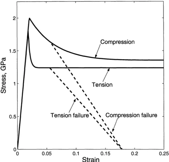
3-1 The solid lines show the stress-strain response in tension and compres-sion (absolute values) for a zirconium-based metallic glass, based on the material parameters listed in §3.1. The dashed lines show the assumed stress-strain curves when modelling failure due to shear localization. 55 3-2 Stress-strain curve from a three-dimensional tension simulation.

Con-tour plots of the equivalent plastic strain keyed to two points on the stress-strain curve are also shown: (a) in the vicinity of the peak, and

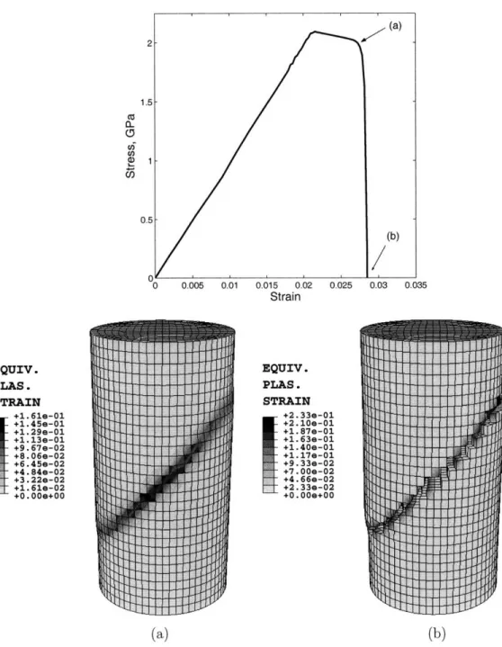
(b) at final failure. ... . ... 56 3-3 Stress-strain curve from a three-dimensional compression simulation

(absolute values). Contour plots of the equivalent plastic strain keyed to two points on the stress-strain curve are also shown: (a) in the vicinity of the peak, and (b) at final failure. ... ... 57 3-4 (a) Finite element mesh consisting of 5000 ABAQUS-CPE4R elements

for two-dimensional simulations of plane-strain tension and compres-sion. (b) Contour plot of initial value of cohecompres-sion. ... ... 58 3-5 Stress-strain curve from a two-dimensional plane-strain tension

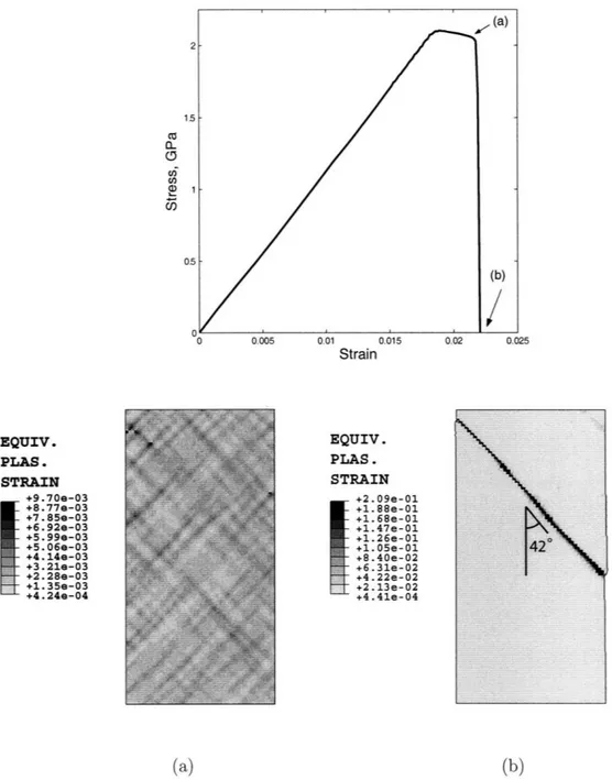
sim-ulation. Contour plots of the equivalent plastic strain keyed to two points on the stress-strain curve are also shown: (a) in the vicinity of the peak, and (b) at final failure. ... . 59 3-6 Stress-strain curve from a two-dimensional plane-strain compression

simulation (absolute values). Contour plots of the equivalent plastic strain keyed to two points on the stress-strain curve are also shown:

3-7 Simulation of bending of a strip of a metallic glass. (a) The strip is clamped between a pair of rigid dies, and then the rigid mandrel is moved upwards to bend the strip about the radius of the upper die.

(b) Deformed strip showing shear bands in the plastically-deformed region (not to scale). (c) Magnified image of a portion of the strip showing contour plots of the equivalent plastic strain. . ... . 61 3-8 Simulation of plane-strain wedge indentation of a metallic glass. (a)

The finite element mesh and indenter geometry. The mesh consists of 25,458 ABAQUS-CPE4R plane strain elements; the mesh density under the indenter is much higher than elsewhere. To approximate a Vickers indenter, the wedge half-angle is chosen to be 680. (b) Mag-nified image of the indented region under the tip showing shear-bands

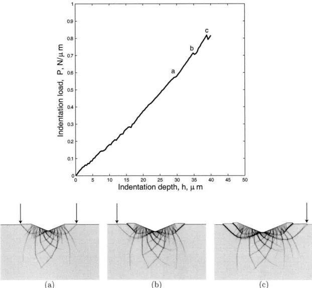
(as evidenced by contour plots of the equivalent plastic strain). ... 62 3-9 Indentation load per unit thickness P, versus indentation depth h

(ab-solute values). Distinct "load-drops" marked as events a, b, and c on the P - h curve, occur when the shear bands indicated by arrows in

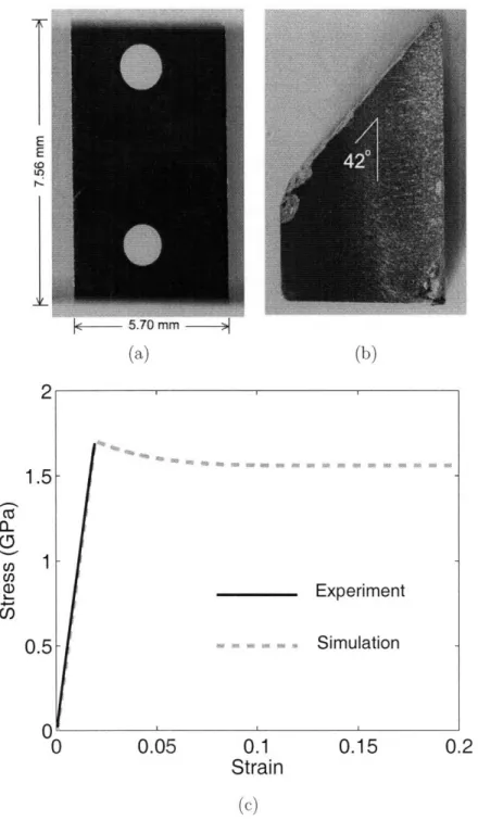
figures (a), (b) and (c) in the bottom panel intersect the free surface. 63 4-1 Simple compression experiment on a Zr-based metallic glass. (a)

Spec-imen between compression platens; the two painted dots were used as markers for an optical strain measurement system. (b) One-half of the fractured specimen. (c) The experimentally-measured stress-strain curve is shown as the solid line. The underlying strain-softening stress-strain curve used in the indentation simulations is shown as the dashed

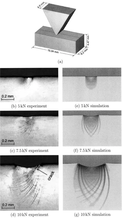
4-2 (a) Schematic of the plane-strain indentation experiment. (b) Front-view of the indenter and the substrate; the two painted dots were used a.s markers for an optical indentation depth measurement system. (c) Rectangular impression left on the surface after indentation. (d) Experimentally-measured P-h curves to load levels of 5 kN, 7.5 kN, and 10 kN are shown as solid lines. The numerically-calculated curves are shown as the dashed lines ... . . . ... .. 77 4-3 (a) Schematic of an indentation experiment on a specimen with a,

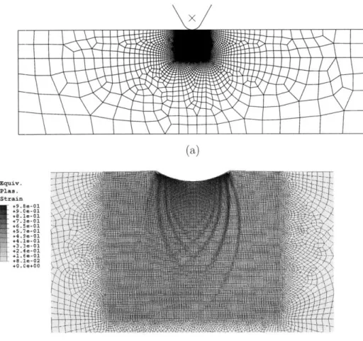
bonded-interface. (b, c, d) Optical micrographs of shear band patterns under the indenter after unloading from load levels of 5 kN, 7.5 kN, and 10 kN. (e, f, g) Corresponding numerical simulations showing contour plots of the equivalent plastic shear strain. . ... . . . 78 4-4 (a) Initial finite element mesh for the plane strain indentation

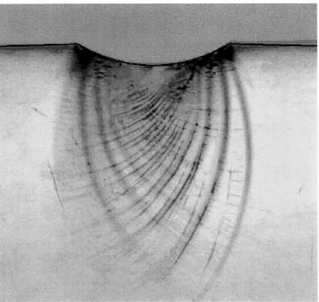
simula-tion. The region of the mesh under the indenter appears black because it has a much higher mesh density. (b) A magnified image of the area under the indenter in the deformed mesh after unloading from a 10 kN simulation. A contour plot of the equivalent plastic shear strain is also shown on this deformed mesh. ... ... . . 79 4-5 Superposition of the contour plot for the equivalent plastic shear strain

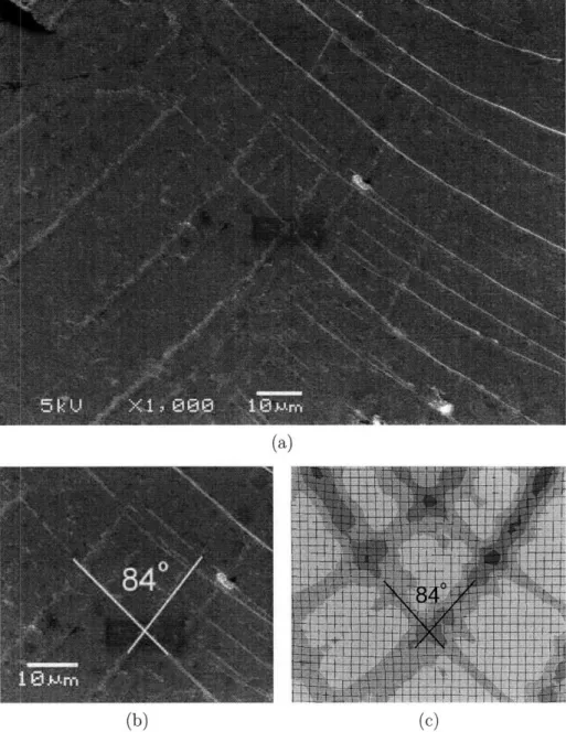
on the corresponding experimentally-observed shear band pattern un-der the indenter for the 10 kN indentation. . ... . . . 80 4-6 (a) SEM image of intersecting shear bands under the indenter; (b) the

angle between two intersecting shear bands is a 84o; (c) contour plot of the equivalent plastic strain from the numerical simulation gives essentially the same angle between two intersecting shear bands. .... 81 4-7 Contour plot of the equivalent plastic shear strain under the cylindrical

indenter showing that plastic flow first takes place at a finite distance beneath the indenter. . ... ... ... 82 4-8 Contour plots of (a) Tresca stress, (b) mean normal pressure, and (c)

5-1 True stress-strain curves for Pd40Ni40P20 from de Hey et al. (1998): (a) Pre-annealed at 564K for 5000 s, then tested at 564K at the differ-ent strain rates indicated in the figure. (b) Pre-annealed at 556K for 120, 720, and 10,000 seconds, respectively, then tested at 556K at a strain rate of

e

seconds, and then subjected to a strain rate increment-and-decrement experiment at 556K. ... ... 109 5-2 Steady state flow stress a,,, as a function of strain rate e at three

different temperatures. The symbols represent experimental results from de Hey et al. (1998), and the lines are from the model. ... 110 5-3 The normalized steady state flow defect concentration as a function

of strain rate at three different temperatures. The symbols represent experimental results from de Hey et al. (1998), and the lines are from

the model ... ... ... ... 110

5-4 The steady state free volume r*, as a function of strain rate at three different temperatures. The symbols represent experimental results from de Hey et al. (1998), and the lines are from the model. ... . 111 5-5 True stress-strain curves for Pd₄₀Ni40P20, pre-annealed at 564K for

5000 s, tested at 564K at different strain rates. The solid lines represent experimental results from de Hey et al. (1998), and the dashed lines are from the model ... ... .. .... .... 111 5-6 True stress-strain curves for Pd40Ni40P20, pre-annealed at 556K for

120s, 720s, and 10,000s, respectively, and tested at 556K and 1.7 x 10-4 _s-1

. The solid lines represent experimental results from de Hey et al. (1998), and the dashed lines are from the model. . ... 112 5-7 True stress-strain curves for Pd40Ni40P20, pre-annealed at 556K for

3600 seconds, and then subjected to a strain rate increment-and-decrement experiment at 556K. The solid lines represent experimental results from de Hey et al. (1998), and the dashed lines are from the model. ... 112

5-8 (a) Finite element mesh consisting of 5000 ABAQUS-CPE4R elements for the two-dimensional plane strain tension simulation. (b) Contour plot of the distribution of the initial free volume... .. ... ... 113 5-9 Engineering stress-strain curve from a two-dimensional plane strain

tension simulation. Contour plots of the equivalent plastic strain keyed to two points on the stress-strain curve are also shown: (a) in the vicinity of the stress peak; (b) when the stress reaches the steady state value. ... . . . ... . . .... . .. . 114 5-10 Simulation of bending of a strip of a Pd-based metallic glass at 556K.

(a) The strip is clamped between a pair of rigid dies, and then the rigid mandrel is moved upwards to bend the strip about the radius of the upper die. (b) Deformed strip showing contour plots of the equivalent plastic strain ... .. . ... . .. . . . . . . 115

5-11 (a) Initial finite element mesh for the axi-symmetric micro hot-embossing simulation. (b) Deformed mesh after the die is reversed. Contour plot of the equivalent plastic shear strain is also shown. (c) A three-dimensional view of the embossed pillar. (d) Die load versus displace-ment during embossing. Observe the sharp increase of the load when the material fully fills the die. . .. . ... ... . . ... . .. .... 116 6-1 (a) An amorphous grain-boundary region "GB" sandwiched between

elastic layers "A". The bottom edge of the sandwiched layer is held fixed, while udenotes the displacement of the top edge (b) A contour plot of the initial cohesion c assigned to the grain-boundary elements before deformation; the initial value of c for each grain-boundary ele-ment was randomly assigned a value from a list which had values of c uniformly distributed between 510 and 590 MPa. .. . . .... . . .. 125

6-2 (a) Shear response of an amorphous grain-boundary region. The bot-tom edge of the sandwiched layer is held fixed, while the top edge is displaced by uto produce a. simple shear deformation. (b) Nominal shear stress versus shear strain response of the grain-boundary region in simple shear, using representative values of material parameters for the amorphous layer. (d) A contour plot of the equivalent plastic strain, showing inhomogeneous deformation in grain-boundary region after a shear strain of 50%. ... ... 126 6-3 (a) Normal traction versus nominal normal strain of the amorphous

laver for u90 and u45. (b) Tangential traction versus nominal shear strain of the amorphous layer for u0 and u45. (c) Failure pattern of the amorphous grain-boundary region subject to normal displacement u90. (d) Failure pattern for u4 5. (e) Failure pattern for uo. . . . . 127 A-1 Schematic of interface between two bodies B+ and B-. ... . 146 A-2 Schematic of yield surfaces for the normal and shear mechanisms. . . 146 A-3 True stress-strain curve for aluminum alloy 6061-T6. . ... 147 A-4 Calibration of Al/Hysol/Al interface response. (a): Geometry of the

specimen used for measuring the traction-separation response in the direction normal to the interface; all dimensions are in mm. (b): Traction-separation curve in the normal direction from experiment, as well as the curve-fit used in subsequent simulations. (c): Geometry of the specimen used for measuring the interface traction-separation response in shear; all dimensions are in mm. (d): Traction-separation curve in the shear direction from the experiment, as well as the curve-fit used in subsequent simulations. ... ... 148

A-5 L-peel experiments: (a): Geometry of the specimen; all dimensions are in mm. (b): Photograph of a deformed specimen in an experiment. (c): Deformed mesh in a corresponding numerical simulation (outline only).

(d): Force versus displacement curves from the experiments conducted at a constant displacement rate of 4 x 10- 3 mm/sec, compared with the corresponding result from the numerical simulation. ... . 149 A-6 T-peel experiments: (a): Geometry of the specimen; all dimensions

are in mm. (b): Photograph of a deformed specimen in an experiment. (c): Deformed mesh in a corresponding numerical simulation (outline only). (d): Force versus displacement curves from the experiments conducted at a constant displacement rate of 4 x 10- 3 _mm/sec, coin-pared with the corresponding result from the numerical simulation for sheet thicknesses of 1.59 mm and 0.79 mm. . ... 150 A-7 Four-point bend experiments on bonded bi-layer edge-notch specimens:

(a): Geometry of the specimen and the four-point bend configuration; all dimensions are in mm. (b): Photograph of a deformed specimen in an experiment. (c): Deformed mesh in a corresponding numerical simulation (magnified 2). (d): Force versus displacement curves from the experiments conducted at a constant displacement rate of 4 x 10-3 mm/sec, compared with the corresponding result from the numerical

simulation. . ... ... 151

A-8 Lap-shear experiments: (a): Geometry of the specimen; all dimensions are in mm. (b): Photograph of a deformed specimen in an experiment. (c): Deformed mesh in a corresponding numerical simulation (outline only). (d): Force versus displacement curves from the experiments conducted at a constant displacement rate of 10- 3 _{mm/sec, compared} with the corresponding result from the numerical simulation for sheet thicknesses of 0.80 mm and 1.59 mm. . ... ... 152

Chapter 1

Introduction

This project focuses on modelling the finite deformation and failure behavior of amor-phous metallic materials. Amoramor-phous metals is of immense fundamental scientific and

technical interest at the present time.

Under slow to moderate cooling rates most metallic materials solidify in a poly-crystalline form; however, under high cooling rates, certain metallic alloys solidify in a disordered form, and such disordered metals are referred to as amorphous metals or

metallic glasses; they are metastable liquids that cannot find their equilibrium

crys-talline state. The first amorphous Au-Si metallic glass was developed in thin ribbon form using a very high cooling rate of 105 - 106 K/s by Klement et al. (1960), but by the late 1980s and early 1990s it was discovered that metallic glasses could be processed at relatively slow cooling rates (1 - 100 K/s) in bulk form in certain multi-component alloy systems due to sluggish crystallization kinetics (e.g., Inoue, 2000; Johnson, 1999, 2002). The current generation of bulk metallic glasses is believed to have many potential applications resulting from their unique properties: superior ten-sile strength (x 2.0 GPa), high yield strain (=2%), relatively high fracture toughness

15 - 25 MPav/¶i, and good corrosion resistance.

When a metallic glass is deformed at ambient temperatures, well below its glass transition temperature, its inelastic deformation is characterized by strain-softening which results in the formation of intense localized shear bands; fracture typically

can be achieved under states of confined compression, such as in indentation exper-iments (cf., e.g., Argon, 1979, 1993; Spaepen, 1977; Donovan, 1988, 1989; Hays et al., 2000; Vaidyanathan et al., 2001; Mukai et al., 2002). The micro-mechanisms of inelastic deformation in bulk metallic glasses are not related to dislocation-based mechanisms that characterize the plastic deformation of crystalline metals. The plas-tic deformation of amorphous metallic glasses is fundamentally different from that in crystalline solids because of the lack of long-range order in the atomic structure of these materials. The computer simulations of Argon and co-workers (cf., e.g., Deng et al., 1989; Argon, 1993) show that at a micromechanical level inelastic deforma-tion in mietallic glasses occurs by local shear transformadeforma-tions in clusters of atoms (a 30 to 50 atoms), and topologically such shear transformations require a local inelas-tic dilatation that produces an elasinelas-tic strain field in the surrounding material, that auto-catalytically then initiates similar shear transformations in neighboring volume elements, leading to the formation of shear bands.

An important consequence of the micro-mechanism of inelastic deformation in amorphous metals is that at the macroscopic level, experimentally-determined yield criteria for inelastic deformation are found not to obey the classical pressure-insensitive Mises or Tresca forms, but show a strong pressure sensitivity of plastic flow (cf., e.g., Donovan, 1988, 1989; Bruck et al., 1993; Lewandowski and Lowhaphandu, 2002). Although the experimental studies mentioned above all suggest a failure of the appli-cability of the classical Mises or Tresca yield criteria, for metallic glasses, they do not conclusively identify the form of the pressure-sensitivity. Recently, Lund and Schuh (2003) have reported on their molecular-dynamic simulations of multiaxial deforma-tion in a model metallic glass. They found that there was a pronounced asymmetry between the magnitudes of the yield strengths in tension and compression. By ex-ploring a variety of biaxial stress states, they numerically probed a plane-stress yield surface for their model metallic glass and found that it was not well-described by tra-ditional pressure-insensitive yield criteria. However, the pressure-sensitive Coulomb-MIohr yield criterion was found to describe the data from their numerical simulations quite well.

the stress required for flow of a granular material; however, the flow rule, that is, the equation which governs the flow behavior for this class of materials, is generally not agreed upon. An attractive two-dimensional (plane-strain) rate-independent flow rule for Coulomb-Mohr materials is the "double-shearing" flow rule (e.g., Spencer, 1964, 1982; Mehrabadi and Cowin, 1978; Nemat-Nasser et al., 1981; Anand, 1983). Recently, Anand and Gu (2000) have generalized this model to three-dimensions; their model includes the effects of elastic deformation, and the typical pressure-sensitive

and dilatant, hardening/softening response observed in granular materials.

In Chapter 2 we further generalize the rate-independent elastic-plastic constitu-tive model of Anand and Gu (2000) to formulate a thermodynamically consistent, finite-deformation macroscopic theory for the rate-dependent elastic-viscoplastic de-formation of pressure-sensitive, and plastically-dilatant materials, and apply it to

model the deformation of amorphous metallic glasses under isothermal conditions. We have implemented our new constitutive model in the finite element program ABAQUS/Explicit (2004) by writing a user material subroutine. Using this numerical implementation of our model, in Chapter 3 we study the response of a metallic glass in tension, compression, strip bending, and indentation, and show that results from our numerical simulations capture major features of corresponding results from physical experiments available in the literature (Anand and Su, 2005).

In Chapter 4 we report our own plane strain indentation experiments on a Zr-based bulk metallic glass. We have measured the corresponding macroscopic load (P) versus indentation depth (h) curves, and studied the evolution of the shear band patterns under the indenter. We shall show that the constitutive model and numerical simulation capability developed previously is capable of producing simulations that

quantitatively compare very favorably against the corresponding experimental results

(Su and Anand, 2006).

The relative low ductility of metallic glasses at ambient temperature makes it dif-ficult to efficiently machine metallic glass raw materials into complex shapes at the ambient temperature. However, like silica glasses, metallic glasses have low viscosities at higher homologous temperatures. Also they can endure a significant amount of plastic strain without failure at this temperature regime. Therefore it is easier to

forge a. metallic glass into desirable shapes at high temperatures. We envision preci-sion forging/embossing will be an important process in manufacturing metallic glass components for applications requiring feature size in the micron range. To make this process more time and cost efficient it is necessary to understand and to be able to simulate the response of a metallic glass at high homologous temperatures.

In Chapter 5 we extend the model developed in Chapter 2 to the high homolo-gous temperature regime and use the numerical capability to study the response of a representative Pd-based metallic glass. Specifically, the response of metallic glass Pd40Ni40P20 in tension at various strain rates and temperatures with different pre-annealing histories is studied. It is shown that results from the numerical simulations compare favorably against corresponding experimental results. The response of this representative metallic glass in a few possible manufacturing processes such as strip bending. indentation and forging is also simulated, which shows the potential capa-bility of this constitutive model in facilitating the design and manufacture of metallic glass components

It is well known that in polycrystalline metals, a substantial increase in strength and hardness can be obtained by reducing the grain size to the nanometer scale (cf., e.g., Gleiter, 1989; Suryanarayana, 1995; McFadden et al., 1999; Jeong et al., 2001; Schuh et al., 2002; Lu et al., 2000). These attributes have generated considerable interest in the use of nanocrystalline (nc) metallic materials (grain sizes less than

100 nm), for a wide variety of structural applications. The hardness, stiffness, strength and ductility of some nc-fcc metals (e.g., Cu, Ni), as measured by microin-dentation and simple tension experiments, have been reported in the recent literature (e.g., Nieman et al., 1991; Sanders et al., 1997; Ebrahami et al., 1998, 1999; Legros et al., 2000; Lu et al., 2001; Torre et al., 2002).

Both physical experiments and atomistic simulations show that for nanocrystalline materials, plasticity induced by dislocation motion inside the grain interiors becomes less significant, whereas separation and sliding of grain boundaries starts to play an important role in the overall inelastic deformation and failure response of these materials (Kumar et al., 2003).

nanocrys-talline metals, as the crystal grain size decreases to zero, in Chapter 6 we extend our amorphous constitutive theory by adding in a cavitation mechanism to model the failure phenomenon caused by the principal and hydro-static stresses. With the revised theory we studied the response of a prototypical amorphous grain-boundary.

Coupled with appropriate crystal-plasticity constitutive model to represent the grain interior, the result obtained in this chapter is applied to study the deformation and failure behavior of nanocrystalline fcc metals (Wei, Su, and Anand, 2006).

Chapter 2

A theory for amorphous

viscoplastic materials undergoing

finite deformations

2.1

Kinematics

With minor modifications for plastic compressibility, the development of the theory in §2.1-:i 2.4 closely follows the work of Gurtin (2002) and Anand and Gurtin (2003).

2.1.1

Basic kinematics

We consider a homogeneous body BR identified with the region of space it occupies in a, fixed reference configuration, and denote by X an arbitrary material point of BR. A motion of BR is then a smooth one-to-one mapping x = y(X, t) with deformation

gradient, velocity, and velocity gradient given by1

F = Vy, v = r, L = grad v = FF- 1. (2.1)

1

Notation: V and Div denote the gradient and divergence with respect to the material point X

in the rejfrence configuration; grad and div denote these operators with respect to the point x in the deformed configuration; a superposed dot denotes the material time-derivative. Throughout, we write Fe - 1 = (Fe)- 1, FP- T = (FP)- T, etc. WVe write trA, symA, skwA, A0, and sym0(A

respectively, for the trace, symmetric, skew, deviatoric, and symmetric-deviatoric parts of a tensor

A. Also, the inner product of tensors A and B is denoted by A - B, and the magnitude of A by

We base our theory on the Kroner (1960)-Lee (1969) decomposition

F = FeFP. (2.2)

Here, suppressing the argument t:

* FP(X) represents a local plastic deformation of the material at X due to "plastic mechanisms" such as the cumulative effects of inelastic transformations resulting from the cooperative action of atomic clusters in metallic glasses in a microscopic neighborhood of X; this local deformation carries the material into - and ultimately "pins" the material to - a coherent structure that resides in the

relaxed space at X (as represented by the range of FP(X));

* FP (X) represents the subsequent stretching and rotation of this coherent struc-ture, and thereby represents the "elastic mechanisms" such as stretching and rotation of the interatomic structure in metallic glasses.

We refer to FP and Fe _{as the plastic and elastic parts of F.} By (2.1)3 and (2.2),

L = Le + FeLPFe-1, (2.3) with

Le = FeFe-1, LP = FPFp - 1. (2.4)

As is standard, we define the elastic and plastic stretching and spin tensors through

D

= symLe,

We = skwLe,

(2.5)

so that :Le = De _{+ We and L}P

= Dp + WP.

With the use of (2.1), equation (2.3) may be written as

grad v = Le

The right polar decomposition of F' is given by

Fe = ReUeU _,

_(2.7)

where Re is a rotation, while Ue is a symmetric, positive-definite tensor with

(2.8)

Ce

Ue

We write

and hence, using (2.2),

J = JeP, where def det Fe, and JP =f det FP.

We refer to

tr LP= tr DP as the plastic dilatation-rate, and note that

JP = JP tr Lp.

For later use, we define the plastic volumetric strain by

def

r7

=

In

P;

(2.12)

2.1.2

Frame-indifference

Changes in frame (observer) are smooth time-dependent rigid transformations of the Euclidean space through which the body moves. We require that the theory be invariant under such transformations, and hence under transformations of the form

y(X, t) -+ Q(t)y(X, t) + q(t)

with Q(t) a rotation (proper-orthogonal tensor) and q(t) a vector at each t. under a change in observer, the deformation gradient transforms according to

F - QF.

L - QLQ

+

QQ

_.

Moreover, FeFP -- QFeFP, and hence since observers view only the deformed

config-urations2

Fee QF ,~ _{and F}P_{is invariant, (2.18)}

and, by (2.4)2

LP is invariant. Also, by (2.4)1, Le _{-- QLeQ}T₊

_QQ

D

--+ QDeQ

_,

_QQT.

(2.19)

(2.20)

QF e --+ QReUe = QVeQ TQRe,

2

That is, the reference configuration and relaxed spaces are independent of the choice of such changes in frame.

and we nmay conclude from the uniqueness of the polar decomposition that

Re -- QRe, Ve -- QVQ , Ue _{is invariant. (2.21)}

2.2

Internal and external expenditures of power

,)We write B(t) = y(BR, t) for the deformed body. We use the term part to denote an

arbitrary time-dependent subregion P(t) of B(t) that deforms with the body, so that

P(t) = Y(PR, t) (2.22)

for some fixed subregion PR of BR. The outward unit normal on the boundary OP of

P is denoted by n.

We assume that power is expended internally by a stress T power-conjugate to

Le, and a microstress TP _{power-conjugate to LP, and we write the internal power as}

4int (P)

=

Here T and TP are defined over the body for all time. The term Je-1 arises because

TP - LP is measured per unit volume in the relaxed space, but the integration is carried out within the deformed body.

The power expended on P by material or bodies exterior to P results from a

macroscopic surface traction t(n), measured per unit area in the deformed

configu-ration, and a macroscopic body force b, measured per unit volume in the deformed configuration, each of whose working accompanies the macroscopic motion of the body. Tfhe body force b is assumed to include inertial forces.3 _{We therefore write the}

external power as

/Vext (P) = t(n) - v da +

J

with t(n) (for each unit vector n) and b defined over the body for all time.

3

Inertial forces result in specific class of external body forces. Granted an inertial frame, in-ertial body forces have the form bil, = -p~. with p(x, t) > 0 the mass density in the deformed configuration.

2.2.1

Consequences of frame-indifference

Consider the internal power Wint(P) under an arbitrary change in frame. In the new frame P transforms rigidly to a region P*, T to T* and TP _{to TP*. If we transform}

the integral over P* _{to an integral over P and use the transformation laws in §2.1.2,} we find that the internal power transforms as

/nt(P*) = j T*. (QLeq T T) + e- 1T* -LP dv.

We require that the internal power be invariant under a change in frame: Wit(P*) =

Wint (P). Since P is arbitrary, this requirement yields the relation

T*. (QLeQT +

QQ

) +

Also, since the change in frame is arbitrary, if we choose it such that

Q

T -- QTQT, TP is invariant. (2.25)

On the other hand, if we assume that

Q

Q

Q

T = TT . (2.26)

Finally, using the symmetry of T, we may write the internal power as

WVint(P) = (T De + Je-lTP LP) dv. (2.27)

2.3

Principle of virtual power. Macroscopic and

microscopic force balances

The theory presented here is based on the belief that the power expended by each independent "rate-like" kinematical descriptor be expressible in terms of an associated

force system consistent with its own balance. But the basic "rate-like" descriptors, namely, v, L', and LP are not independent, as they are constrained by (2.6), and it is

not apparent what forms the associated force balances should take. For that reason, we determine these balances using the principal of virtual power.

2.3.1

Principle of virtual power

Assume that, at some arbitrarily chosen but fixed time, the fields y, Fe (and hence F and FP) are known, and consider the fields v, Le, and LP as virtual velocities to

be specified independently in a manner consistent with (2.6); that is, denoting the virtual fields by ir, L•, and LP to differentiate them from fields associated with the actual evolution of the body, we require that

grad r = Le + FeLPFe-1. (2.28)

More specifically, we define a generalized virtual velocity to be a list

S= (ILe,

L),

consistent with (2.28).

Writing

Wext(P, V) =

t(n)

da

+

b

(2.29)

int (P, V) =

j(T

respectively, for the external and internal expenditures of virtual power, the principle

of virtual power is the requirement that the external and internal powers be balanced:

given any part P,

2.3.2

Macroscopic force and moment balances. Microforce

balance

To deduce the consequences of the principle of virtual power, assume that (2.30) is satisfied. In applying the virtual balance (2.30) we are at liberty to choose any V consistent with the constraint (2.28).

Consider a generalized virtual velocity with LP = 0, so that grad 9 = Le. For this choice of V, (2.30) yields

p t(n) .- da+ p b v dv = T gradidv.

and, using the divergence theorem,

I

Since this relation must hold for all P and all 9, standard variational arguments yield the traction condition

t(n) = Tn, (2.31)

and the local force balance

div T + b = 0. (2.32)

Therefore, recalling (2.26), the symmetric stress T plays the role of the Cauchy stress,

and (2.32) and (2.26) represent the macroscopic force and moment balances.

To discuss the microscopic counterparts of these results, we next choose 9 - 0. Then the external power vanishes identically, so that, by (2.30), the internal power must also vanish. Moreover, by (2.28), Le = -FeLPFe-1, and hence

(je-1 (TP - JeFeTTF-T) .LP dv= 0.

the microJorce balance

= Tp, where Te de2 JF TTF e-T

. (2.33)

This balance characterizes the interaction between internal forces associated with the elastic response of the material and internal forces associated with inelasticity.

2.4

Dissipation inequality (second law)

We consider a purely mechanical theory based on a second law requiring that the

temporal increase in free energy of any part P be less than or equal to the power expended on P. Let

4

SPJe-1

dv

Wext (P) =

Wint

(P).

(2.34)

Since J-ldv with J = det F represents the volume measure in the reference con-figuration, and since P = P(t) deforms with the body, we find, using (2.11) and

(2.12),

j

OJe-1

dv

-=

JPJ-1

=

JPJ-1

(j + V (trLP))J

1

dv.

Thus, since P is arbitrary, we may use (2.27) to localize (2.34); the result is the local

dissipation inequality

S- JeT - De - TP L + trLP < 0. (2.35)

2.5

Constitutive theory

The macroforce balance, the microforce balance, and the dissipation inequality are basic laws, common to large classes of elastic-plastic materials; we keep such laws distinct from specific constitutive equations, which differentiate between particular

materials. We view the dissipation inequality (2.35) as a guide in the development of a suitable constitutive theory. In this regard we do not seek the most general

consti-tutive equations consistent with the dissipation inequality; instead we develop special

constitutive equations close to those upon which the classical theories of plasticity are based.

2.5.1

Constitutive equations

We introduce a list of n scalar internal state-variables on experience with existing theories assume that4

T

_{= (Fe ),}

Under a, change in frame Fe -- QFe _{and T --+ QTQT,}

and ( are invariant; thus, using a standard argument, reduces (2.36) to the specific form

S= ((1,2, .. . n), and based

(2.36)

while LP, Tp and the scalars r we see that frame-indifference

The following definitions phous) material (Anand and

T = ReT(Ue, ,)ReT, T p = TP(Lp , _{T, (),}

SZ= h'(LP, n, ().

help to make precise our Gurtin, 2003):

(2.37)

notion of an isotropic

(amor-(i) Orth- = the group of all rotations (the proper orthogonal group); 4

To avoid an overly complex presentation, our constitutive equations have been taken to de-pend on FP only through the plastic volumetric strain qr, and from the outset we have neglected a dependence of the free energy, /,, and the Cauchy stress, T, on the internal variables (.

(ii) the referential symmetry group Gref is the group of all rotations of the reference configuration that leave the response of the material unaltered;

(iii) the relaxed symmetry group Grel is the group of all rotations of the relaxed space that leave the response of the material unaltered.

We refer to the material as isotropic (amorphous) (and to the reference and relaxed spaces as undistorted) if

Gref = Orth+, Grel = Orth+, (2.38)

so that the response of the material is invariant under arbitrary rotations of the reference and relaxed spaces.5

We now discuss the manner in which the basic fields transform under such trans-formations, granted the physically natural requirement of invariance of the internal power (2.27), or equivalently, the requirement that

T De and TP -L be invariant. (2.39)

Let

Q

Fp -- FPQ and Fe is invariant, (2.40)

so that, by (2.3), Le_{, and (hence) D}e_{, and L}P _{are invariant. We may therefore use} (2.39) to conclude that T and TP are invariant.

On the other hand, let

Q

Fe -+ FeQ and F -+ QT F , (2.41)

and hence (2.3) yields the transformation law LP -- QTLPQ, and the invariance of Le_{, so that D}e

is invariant. Finally, (2.39) yields the invariance of T and the

transformation law TP -' QTTPQ.

5_{For metallic glasses this notion attempts to characterize situations in which the material has a}

We henceforth restrict attention to materials that are isotropic (amorphous) in the sense that the constitutive relations (2.36) (or equivalently, (2.37)) are invariant under all rotations of the reference configuration and, independently, under all rotations of the relaxed spaces.

Applying the former we find that our constitutive equations (2.37) are invariant to all rotations of the reference configuration.

Next, let

ce = FeTFe = (Ue)2,

and, in (2.37), replace Re by FeUe-~ and Ue by v-C; this reduces (2.37) to

V

=

O(Ce

1),

T = FeT(Ce,

7)Fe

(2.42)

TP = TP(LP, 9,

~ h'(LP,

7,

~).

Our final step is to consider invariance under rotations of the relaxed configuration using the transformation rules specified in the paragraph containing (2.41). Under a rotation Q of the relaxed space,

Ce

_{_ Q}

and the response functions

4,

2.5.2

Thermodynamic restrictions

With a view toward determining the restrictions imposed by the local dissipation

inequality, note that

UCe +y y7

Using the symmetry of 80l/&Ce

-C = (2 FeTFe) 2Fe F eT Le 2 e Fe De

Thus, using (A.24) and the result above,

=2 Fe FeT .De + _

1

YCe

a

),

If we substitute (2.42) and (2.43) into the local dissipation inequality (2.35), we find that

Fe (2 • JeT(C, )) Fe -.De- T_ (LP, q, (1+ -IP < 0. (2.44)

This inequality is to hold for all values of Ce, De_{, LP, , and (. Since D}e _appears linearly, its "coefficient" must vanish. Thus Je T= 2 0*//Ce, and we are led to the following constitutive relation for the stress:

T = 2Je-lFe Fe. (2.45)

Also, defining

Sdef )1 (2.46)

Y"(Ce LP , eTP(LP,P,) - (Ce,) + (2.46)

we must have

YP(Ce, LP, ,), LP > 0. (2.47)

The left side of (2.47) represents the rate of energy dissipation, measured per unit volume in the relaxed space. To rule out trivial special cases, we assume that the material is strictly dissipative in the sense that

YP(Ce, LP, 7, () - L > 0 whenever LP ý 0. (2.48)

In light of the dissipation inequality (2.47), we refer to YP as the dissipative flow

2.5.3

Flow rule

A central result of the theory-which follows upon using (2.46) and the microforce balance (2.33)--is the flow rule

T - ((Ce ) + (C'77 1 = YP(Ce, LP, , ). (2.49)

Using the definition (2.33)2 for T' in (2.45), we find that

Te =

2

Ce

(2.50)

aCe

We note that since 4(Ce, rj) is an isotropic function of its arguments, the principal

di-rections of &0(Ce, 77)/Ce coincide with those of Ce, and hence for isotropic materials

the tensor T' is symmetric.

Hence, defining the symmetric stress E by

E d= Te e( Ce' ) 1, E = E , _(2.51)

we may rewrite the flow rule (2.49) as

E = YP(Ce, LP, 1 , (). (2.52)

2.6

Specialization of the constitutive equations

The constitutive restrictions derived thus far are fairly general. With a view to-wards applications we now simplify the theory by imposing additional constitutive assumptions based on experience with existing theories of viscoplasticity.

2.6.1

Invertibility assumption for the flow rule

In classical theories of plasticity, the flow rule is usually specified as an equation for the plastic velocity gradient LP in terms of a suitable stress measure and other internal variables. Accordingly, we assume that for fixed state (Te, E , 17, ý), the dissipative

flow stress function YP is invertible, so that we may write

LI = LI(E, T, )

In this case, the dissipation inequality (2.48) may be written as

E -LP(E,,

) > 0 for L

0O.

Since the function YP is isotropic, we assume that

function of its arguments.

the function LP is also an isotropic

2.6.2

Free energy function. Elastic constitutive equations

Let

3 3

Ue = A Ce= ~rer, A2 ~er ra (2.55)

0=1 a=l

be the spectral representation of Ue and Ce, respectively, with {AI a = 1, 2, 3} the positive eigenvalues, and {rola = 1, 2, 3} the orthonormal eigenvectors of U'. Then, the isotropic free energy function may be expressed as a symmetric function of the principal stretches A):

O(Ce,

7)=

(A , A',

A', I).

(2.56)

Restricting our attention (for now) to the case of distinct eigenvalues {Ae ja = 1, 2, 3}, and using the chain rule we obtain

(ce

E)

a=l

al aAe

Qe

a

Then, since A' = and A,2 =

r~.

Te = 2C

O(Ce)

=

e

r0

ro.

a=1 a

(2.57) (2.53)

Let

3

Ef

Ee =f

E

ro

r.

a=l

denote the symmetric logarithmic elastic strain tensor, with principal logarithmic

elastic strains

Ea d In ln . (2.59)

Then, (2.57) may be written as

3

T =e E ra ®rc, (2.60)

from which we note that for isotropic materials the symmetric stress measure Te is power-conjugate to the logarithmic elastic strain.

Thus, for isotropic materials we may replace the free energy function 4(A~, , A~, rA ) by

(e, e)

with the stress measure Te _{given by}

e

89V(E

'77)

Te = (E (2.61)

OEe Recalling (2.33)2, we note that for isotropic materials

We FeS(JWT)FJf e -s ReT(JeT)Re . (2.62)

To describe the elastic response of the solid we consider the following simple generalization of the classical strain energy function of infinitesimal isotropic elasticity, in which we replace the infinitesimal measure of elastic strain by the logarithmic measure of finite elastic strain (Anand, 1979):

G(E,

where

G=G(ý) >0, K =~K(r,)>0 (2.64)

are the elastic shear and bulk moduli, which we have assumed to depend on plastic volumetric strain rl. In this case the constitutive equations for the stress becomes

Te = 2GEe + K (trEe)1. (2.65)

2.6.3

Kinematical hypothesis for plastic velocity gradient.

Internal variables

We assume that plastic flow occurs by shearing accompanied by dilatation (or com-paction) relative to some slip systems. Each slip system is specified by a slip direction s(" ) , and a slip plane normal m(a) (we label slip systems by integers a), with

s(a) . m(a) = 0,

Is(a), Im(a)I

and we take the plastic stretching to be made up of shearing rates v(a) on the set of potential slip systems, and assume that this shearing is accompanied by shear-induced

dilatation rates 6(a) in the directions normal to the shear directions. That is, the total plastic velocity gradient is taken as

LP

E LP(L),}

L (Q) = v(a)(s(a) ® m(M)) + J(a)(m(a) & m(a)), (a) > 0 (2.67)

where 0 is a dilatancy function. Positive values of/3 describe plastically dilatant behavior, while 03 < 0 describes behavior that is plastically compacting.

For an amorphous isotropic material there are no preferred directions other than the principal directions of stress, and accordingly we consider potential slip systems with respect to these principal directions of stress. The symmetric stress E has the

spectral representation

3

E

~

=

i

i

®

e6.

(2.68)

i= 1

where {aIoi 1= 1, 2, 3} are the principal values, and {f6i = 1, 2, 3} are the orthonormal principal directions of E. We assume that the principal stresses {oaii = 1, 2, 3} are strictly ordered such that

U1 _2 2 _3. (2.69)

First, consider potential slip in the (61, e3)-plane. Let (s(`), m(`)) denote a po-tential slip system lying in this plane and oriented such that s(c) makes an angle 6' with respect to the 61-axis

s(

a)

and let

-(a)(V) = s(O) -

Em

and a(a)(19) = _m (a) .Em (a),

denote the resolved shear stress and compressive normal traction for such a system. Then, introducing an internal variable Iu > 0 called the internal friction coefficient, we define the quantity

def

= arctan p (2.70)

called the angle of internal friction, and assume that any given instant for a fixed stress E, shearing is possible only on those slip systems for which

f(0)= {r(0) - (tan0) )a(,)},

is a, ma.imum with respect to V (Coulomb, 1773). It is easily shown that f(,9) is a maximum for

6=

+

.

(2.71)

which are symmetrically disposed about the maximum principal stress direction: s(l) _{= cos 6}

1 + sin 9•3, m( 1 ) = sin161 - cos 63,

s(2 ) = cos

6

091

with

S= (r/4) + (/2).

In an entirely analogous manner, the slip systems in the (i 1,62)-plane are

s( 3 ) = COS't1 + sin d62,

s( 4 )

= cos d•6 - sin Ve62,

while those in the (62, 63)-plane are

s(5) = cos

ie

+

796

s(6) = cos 0e2 - sin

06

Thus, the total velocity gradient is made of the six potential slip systems:

m( 3 ) = sin l 961 - cos l962, m(4) = sin

061

06.

m( 5 ) _{= sinl}

₆

2 - COS 9

0

d63.

up of contributions from shearing on each

6

LP = E V(a)

{

Om(a) 0

}

a=l

(2.76)

The shearing rates v@) ( are taken to be constitutively prescribed by a flow equation

as follows:

QT() ) 1/rn

s(a) = V0 > 0, (2.77)

c + pa(a)

where we have introduced another internal variable c > 0, called the cohesion (Coulomb,

1773). Also, vo > 0 is a reference plastic shear strain rate, such that v(") = vo when

7(0) = c + pa(

a

0 is a strain-rate sensitivity parameter. For v' > 0, the

flow equation (2.77) may be inverted to read

T (a) = (Cu(+)) ( \ V( V( m

2/

(2.75)

Thus, it is clear that the limit m -~ 0 renders the theory rate-independent.6

The dissipation inequality (2.54) requires that

6

E

-

L

[(a)

-

_3

a( )]

V)

> 0,

(2.79)

0=1

whenever plastic flow occurs. On physical grounds we require that

[T(a) - ( )] (a) > 0 _{for each a; (2.80)}

thus, whenever v(Q) > 0, we must have

[-(a) - • (0)] > 0, (2.81)

which is a, restriction that the dilatancy function 3 must satisfy.

We emphasize that we do not assume that p = 0, which (using classical terminol-ogy) would correspond to an associated/normality flow rule.

Straight-forward calculations show that the resolved shear stresses and compres-sive normal tractions on the slip systems are given by

r(1.2) L sin

(29)(a1

V

(34) sin(2)(a - a2), ( 3,4 ) -

(2)(

._(Ul + _r. 1 cos(2,d) (or (2.3))

S(5,6) = ₁ sin(279)(a_sin 2 - C73), o(5,6) = -' _{2 2+ a'} COS(2')( 2 -

a

3)+ 1 cos(2 d) _93)

Thus, from (2.77) we note that in the case of distinct principal stresses

,1) = (2) ( 3 ) = (4 ) , V(5) = V(6) if O1> > 2 > (73,

(2.83)

and in situations when the principal stresses are not distinct we have

v1,(1) = v(2) = (3) = U(4), = -(5) V(6) = 0 if 0a > 02 = U3,

(2.84)

'More elaborate forms for the dependence may be considered, but a simple power-law rate-dependence makes the structure of our theory more transparent.

1, ( 1 )

- V( 2 ) = V(5 ) = V( 6 ), (3 ) = (4 ) _{= 0,}

if U1 = U2 > U3, (2.85) and

S(1) = (2) = (3) = (4) = (5) (6)

0

(2.86)

Remark 1: When al > a2 = a3, 62 and

63

per-pendicular to 61, and we have an infinite number of potential slip systems with slip

directions s(a) lying on a cone with axis e1 and a semi-angle 9 = {(7r/4) + (0/2)}.

In enumerating our slip systems we choose an arbitrary pair of orthonormal vectors

(62, 63) perpendicular to 61; this choice, and therefore the choice of slip systems is

clearly non-unique. A similar remark concerning a non-unique choice of slip systems holds when a₁ = U2 > U₃.

Remark 2: On account of (2.83), (2.84), (2.85), we note the important result that in this flow rule for isotropic materials, the plastic spin vanishes, W P = 0.

2.6.4

Evolution equations for internal variables. Dilatancy

equation

The internal variables ( of the model are the cohesion c and the internal friction p = tan 4, for which we need to prescribe evolution equations, and we also need to specify a constitutive equation for the dilatancy function 0, which determines the evolution of the volumetric plastic strain r.

For the amorphous metallic materials under consideration we adopt the following special forms:

(1) Internal friction: The internal friction [ is taken to be a constant,

I = I• > 0. (2.87)

(2) Evolution of rl. Dilatancy Function. Evolution of c: The free-volume for an amorphous material is defined to be the difference between the actual specific volume of the material and the specific volume if the material was in a state of dense random packing. A key feature controlling the plastic deformation of