Controller design for precision magnetic bearings

Controller Design for Precision Magnetic Bearings

by

Tetsuya Kubota

B.S., Mechanical Engineering (1986) Tokyo Institute of Technology M.Eng., Mechanical Engineering (1988)

Tokyo Institute of Technology

Submitted to the Department of Mechanical Engineering in Partial Fulfillment of the Requirements for the degree of

Master of Science at the

Massachusetts Institute of Technology May, 1997

@Tetsuya

The author hereby grants to MIT permission to reproduce and to distribute publicly copies of this thesis document in whole or in part.

Signature of Author

Department of Mechanical Engineering May 9, 1997 Certified by .. s7~

/I

JUL 2 . 1997

Engr

-~rr

Controller Design for Precision Magnetic Bearings

by

Tetsuya Kubota

Submitted to the Department of Mechanical Engineering on May 9, 1997 in partial fulfillment of the

requirements for the degree of Master of Science ABSTRACT

For some uses of magnetic bearings such as precise positioning of a rotor, the ability to control the rotor actively is essential. However, the consideration of performance robustness is required for this application because of unknown parameters, unpre-dictable disturbances, and the nonlinearity of magnetic force. This thesis focuses on the achievable robustness of the system designed by linear theories and perfor-mance comparison between the linear approach and adaptive approach. First, the examples of the controller design for the magnetic bearing using the LQG design,

H, design, LQG/LTR design, and tu-synthesis are presented to show how the linear

theories achieve stability and/or performance robustness. Second, the limitations of linear controllers for the system with uncertainties are evaluated by using singular value plots and structured singular value plots. Furthermore, it is revealed that when the system reaches its limit, the gain of the controller becomes extremely high; there-fore, it should be avoided. The effect of the order reduction of the controller is also examined. Then, the robustness of the linear controller and adaptive controller using local function estimation is compared by simulations. The results show the adaptive controller can deal with wider range of uncertainties than the linear controller can, but high frequency unmodeled dynamics impose limitations on adaptive gain.

Thesis Supervisor: Dr. Kamal Youcef-Toumi

Acknowledgement

First, I would like to thank my thesis adviser. His support and guidance have led me to the proper direction in this research. I also want to thank all the students I worked with at the mechatoronics reseach laboratory. Particulary, the advice from Jake and T.-J. much helped me at the early stage of the work. I am also thankful to Kawasaki Heavy Industries, which gave me the chance to study at MIT. Finally, I thank to my parents and wife. Without my wife's support, I could not have completed my thesis.

Contents

1 Introduction

1.1 Motivation and Background . . . . 1.2 Scope and Contents of the Thesis . . . . .

2 Control of Magnetic Bearings with Linear 2.1 Introduction...

2.2 Model of the Magnetic Bearing 2.3 Design Examples ... 2.3.1 LQG Design ... 2.3.2 Hoo Design ... 2.3.3 LQG/LTR Design.... 2.3.4 p-Synthesis ... 2.4 Summary ... 14 14 16 Controllers 19 20 . . . . 22 . . . . 23 . . . . 24 . . . . 32 . . . . 36 . . . . 42

3 Limitations of Linear Controllers

3.1 Introduction.. . . . ... ... .. . .. . . . . ... . 3.2 Achievable Performance with Limited Bandwidth . . . . 3.3 Limitation with Parameter Uncertainties . . . . 3.4 Adverse Aspects of Large Uncertainties . . . . 3.5 Limitation with Parameter Uncertainties and Bandwidth Limitation . 3.6 Order Reduction of the Designed Controller . . . . 3.7 Using Prefilters to Reduce Control Input . . . . 3.8 Sum m ary . . . . 45 45 46 48 51 56 63 65 68 -

-4 Control of Magnetic Bearings with an Adaptive Approach 71

4.1 Introduction ... ... 71

4.2 Nonlinear Model of the Real Magnetic Bearing . ... 72

4.3 Equivalent Uncertainties of the Nonlinearity . ... 74

4.4 Adaptive Control Using Local Function Estimation . ... 75

4.5 Reference Model and Equivalent p-Synthesis Design . ... 78

4.6 Nonlinear Effect on the System with the Linear Controller and Adap-tive Controller ... ... .. 80

4.6.1 Effect of Large Displacement . ... 82

4.6.2 Effect of Gravity ... ... 83

4.7 Effect of High Frequency Unmodeled Dynamics . ... 86

4.8 Summary ... ... 91

5 Conclusions 95 A Design Programs using MATLAB 97 A.1 LQG Design ... . ... 97

A.2 H, Design ... . ... ... 97

A.3 LQG/LTR Design ... . .... ... 99

A.4 p-Synthesis ... ... . ... 100

List of Figures

Cross section of the turbo-pump . . . . .

Schematic of the thrust bearing . . . . Structure of an LQG controller . . . . .

Time response of the LQG designed system. Frequency response of the position sensor. Frequency response of the real system... Time response of the LQG designed system. Mixed sensitivity H, design.. . . . . Desired sensitivity function . . . . .

Multiplicative uncertainty . . . . .

Necessary robustness bound . . . . Sensitivity function of the H, designed system. 2.1 2.2 2.3 2.4 2.5 2.6 2.7 2.8 2.9 2.10 2.11 2.12 2.13 2.14 2.15 2.16 2.17 2.18 2.19 2.20 2.21 . . . . . 20 . . . . . 21 . . . . . 23 . . . . .. . 24 . . . . . 26 . . . . . 26 . . . . . 27 . . . . . 28 . . . . . 29 . . . . . 29 . . . . . 30 . . . . . 31 ed system. ... 31 . . . . . 32 Time response of the H, designed system with the sensor dynamics.

Sensitivity function of the filter loop . ... Closed-loop transfer function of the filter loop . ... Sensitivity function of the LQG/LTR designed system. ...

Closed-loop transfer function of the LQG/LTR designed system. . .

Time response of the LQG/LTR designed system . ...

Time response of the LQG/LTR designed system with the sensor dy-namics. ...

Closed-loop transfer function of the Ho design Time response of the H, designed system. . . _...

2.22 Generalized robust control design problem. .... 2.23 2.24 2.25 2.26 2.27 2.28 2.29 3.1 3.2 3.3

Parametric uncertainty of the system . . . . Block diagram of the p-synthesis structure . . . . . Structured singular values before D-scale fitting. . . D-scales and the fitted 5th order curves for A,. . . D-scales and the fitted 5th order curves for A2. . .

Structured singular values after the D-scale fitting. Sensitivity function with the various rotor masses.

Maximum singular values of Twz(s) ...

Achievable sensitivity functions with various w,.-Closed-loop transfer function of the systems ...

3.4 Structured singular values with various uncertainty ranges.. 3.5 Step responses of the system designed for m = 3.0 - 4.5

various m . . . .

kg with

3.6 Sensitivity functions designed for m = 3.0 ' 5.0 kg with various m.

3.7 Step responses of the system designed for m = 3.0 - 5.0 kg with various m . . . . 3.8 Gain plot of the controller designed by p-synthesis . . . . .

3.9 Increase of the maximum controller gain with the increase of the mass uncertainty. . . . . 3.10 Step response and the control input of the system designed for m =

3.0 - 4.5 kg . . . . 3.11 Step response and the control input of the system designed for m =

3.0 - 4.0 kg .. . . . . . . . . . 38 . . . . . 39 . . . . . 40 . . . . . 41 . . . . . 41 . . . . . 42 . . . . . 43

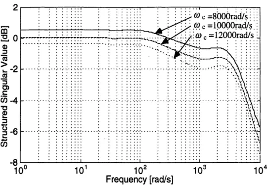
3.12 Step response and the control input of the system designed for m = 3.0 - 3.5 kg... . ... 56 3.13 Concept of p-synthesis with bandwidth limit. . ... . 57 3.14 Structured singular values of the system designed for m = 3.0 - 4.5

kg and various w... .. 58 3.15 Sensitivity functions of the system designed for w, = 20000 rad/s. . . 59

3.16 Closed-loop transfer functions of the system designed for w, = 20000 rad/s. ... .. 59 3.17 Sensitivity functions of the system designed for w, = 10000 rad/s. . . 60 3.18 Closed-loop transfer functions of the system designed for w~ = 10000

rad/s. ... .. 60 3.19 Step responses and the control inputs of the system designed for w~ =

10000 rad/s . . . . 61 3.20 Structured singular values of the system designed for m = 3.0 - 4.0

kg and various w... .. 62 3.21 Structured singular values of the system designed for m = 3.0 - 3.5

kg and various wc... .. 62 3.22 Diagonal of the gramian of the balanced-realized controller ... 64 3.23 Gain plot of the reduced controller and original controller. . ... 65 3.24 Structured singular value plot of the system with the reduced and

original controller ... ... .. 66 3.25 Sensitivity functions of the system with the reduced controller. .... 66 3.26 Gain plot of the reduced controller and original controller. . ... 67 3.27 Structured singular value plot of the system with the reduced and

original controller . ... ... 67 3.28 Concept of a prefilter ... . ... 68

3.29 Prefiltred step input. ... 69 3.30 Step responses and the control inputs of the system with the prefilter. 69

4.1 3-D plot of the magnetic force. . ... ... 73 4.2 Adaptive control scheme using local function estimation. ... 77 4.3 Sensitivity function of the reference model and performance bound. . 79 4.4 Structured singular value plot of the designed system... . 81 4.5 Sensitivity function of the designed system with m = 2.2, 3.0, and 4.5

kg . ... ... ... .. 81 4.6 A 10-pm step response of the reference model... . . . 82 4.7 Step responses of the system with a p-synthesis controller. ... . 82 4.8 100-pm step responses of the system with the linear controller with

m = 2.2 and 4.5 kg... 84 4.9 200-pm step responses of the system with the linear controller with

m = 2.2 and 4.5 kg... ... .. 84 4.10 100-pm step responses of the system with the adaptive controller with

m= 2.2 and 4.5 kg... 85 4.11 200-pm step responses of the system with the adaptive controller with

m = 2.2 and 4.5 kg... 85 4.12 10-pm step responses of the system with the linear controller with

m = 2.2 and 4.5 kg (g = 4.9 m/s2) ... 87 4.13 10-pm step responses of the system with the linear controller with

m = 2.2 and 4.5 kg (g = 9.8 m/s2)... 87 4.14 10-pm step responses of the system with the adaptive controller with

4.15 10-tm step responses of the system with the adaptive controller with

m = 2.2 and 4.5 kg (g = 9.8 m/s2). ... 4.16 Model of the rotor elasticity. . . . ...

4.17 Transfer function of the magnetic bearing with the rotor elasticity. . 4.18 Uncertainty by the rotor elasticity and the stability bound ...

4.19 Step response of the system with cl = 100 Ns/m controlled by the adaptive controller (y = 1 x 107). . ...

4.20 Step response of the system with cl = 100 Ns/m controlled by the adaptive controller (7 = 1 x 106) . . ...

4.21 Step response of the system with cl = 170 Ns/m controlled by the adaptive controller (y = 5 x 108). . . ...

4.22 Step response of the system with cl = 170 Ns/m controlled by the adaptive controller (y = 6.5 x 10). . ...

Chapter 1

Introduction

1.1

Motivation and Background

As a requirement of machines becomes faster and more precise, conventional design methods or machine elements may not be able to achieve the requirement. In this case, we must opt for an unconventional, yet practical approach to achive the requirement. Even though magnetic bearings are not as widely-used as other conventional bear-ings, they have been used in several applications because of their distinctive features. No-contact nature may be the most attractive feature of magnetic bearings. Because there is no friction, magnetic bearings are used for high rotating speed machines such as fly-wheels and turbo-pumps. Also, because no lubrication is necessary, they are used for maintenance-free machines, high speed machines in high temperature envi-ronments, high speed machines in vacuum, and machines in clean rooms. For these applications, especially for industrial applications, many research and development works have been done, and magnetic bearings are widely in use.

There is another attractive feature in magnetic bearings. The fact that magnetic bearings are actively controlled provides some useful applications. One possible ap-plication is for machines that need high speed rotation and precise positioning of the rotor simultaneously. Precise machine-tool spindles and the joints of high-speed, high-precision robot manipulators may be achieved by magnetic bearings. Active con-trol also makes force concon-trol and impedance concon-trol of moving parts possible. This feature is difficult to achieve by other conventional bearings such as ball bearings or

air bearings; therefore, using magnetic bearings largely enhances the machine's capa-bility. However, due to the nonlinearity of magnetic force and nature of instability, the use of magnetic bearings for precise machines requires more effort on designing a control system than just making the rotor levitate for the bearing purpose. Unknown factors, such as unknown load, unmodeled dynamics, or unpredictable disturbances may cause the performance degradation of the system, and to precise machines, it is not acceptable. Nevertheless, the research in the area of precise control of magnetic bearings has not yet been well explored.

In the past decade, modern control theories have evolved to deal with the uncer-tainties in systems. This development is driven by the fact that in real systems, there are many unknown factors, and without considering these factors in the design pro-cess, the closed-loop system often fails to be stabilized, or the resulting performance becomes much poorer than expected. This fact can also be applied to the control of magnetic bearings. However, the recent development of robust control theories has enabled us to design a controller that achieves the desired performance even when uncertainties exist. Moreover, these theories are now readily available as computer aided design tools [1][2]. Nonami et al. applied p-synthesis to the control design for a magnetic bearing and succeeded to robustly control the flexible-rotor magnetic bear-ing system [3]. Even though this proves that the linear robust control theory can be applicable to the real system with uncertainties, fixed gain linear controllers cannot always achieve the desired performance, and knowing the limitation of the controller designed by p-synthesis is as important as the design procedure itself. Moreover, in precise magnetic bearings, the system is affected by nonlinearity because the operat-ing point changes. However, the effect of the nonlinearity is not analyzed in [3].

Because of the strong nonlinearity, other approaches than linear controllers have been applied to magnetic bearings. For example, Shinha et al. applied sliding mode

control to the magnetic bearing even though the report does not include experimental results [4]. Yeh developed an adaptive control method using local function estimation and successfully controlled the rotor of the turbo-pump with magnetic bearings [5]. These results indicate that nonlinear approaches can deal with the strong nonlinearity of magnetic bearings and may be able to achieve performance robustness for precise control.

With these choices of control methods, we must analyze the advantages and dis-advantages of these methods in order to design a proper controller. Generally, linear controllers are most widely used and can be applied easily. However, in some cases, other methods, such as adaptive controllers, far more exceed linear controllers in terms of achievable performance. Astrim et al. discussed this issue in their literature [6]. However, it does not mention the limitation of robustness of linear controllers. With the advent of p-synthesis now, we are able to judge the limitation of linear con-trollers applied to the system with uncertainties. One of the purposes of this thesis is to provide the information about the methodology and examples of the limitation of the magnetic bearing system designed by p-synthesis along with the comparison with an adaptive method. This information helps control designers choose the proper control structure.

1.2

Scope and Contents of the Thesis

This thesis contains three schemes: linear control design examples, evaluation of limitations of linear controllers, and comparison of the linear approach and adaptive approach. By using design examples, it is shown how linear controllers are able to deal with the uncertainties that exist in the magnetic bearing system. The design methods used in this part are LQG, Hooc, LQG/LTR, and M-synthesis, and in these

methods, only p-synthesis can deal with performance robustness. Even though the design process of these theories is not trivial, commercially available CAD programs exist, and all four controllers are designed using these programs. The program codes to calculate the controllers are listed in the Appendix.

The limitation of linear controllers for the system with uncertainties are evaluated by singular value plots or structured singular value plots. In this part, the limitation by the bandwidth limit of the closed-loop system, limitation by the uncertainty of the rotor mass, and limitation by both the uncertain mass and bandwidth limit are evaluated. Also, as the adverse aspects of the robust linear controllers, high gain and high order of the designed controllers are discussed, and the effect of order reduction and prefilters is presented.

The effect of nonlinearity on the performance of the system with uncertainties is discussed by using nonlinear simulations. In this part, the adaptive control us-ing local function estimation, by which the turbo-pump with magnetic bearus-ings are controlled successfully, is briefly described to compare the linear approach and adap-tive approach. Because of the strong nonlinearity of magnetic force, the system with the linear controllers may not be able to deal with the nonlinearity whereas with the adaptive approach, which estimates the nonlinear function as well as unknown disturbances, is not affected by the nonlinearity. Also, the effect of high frequency unmodeled dynamics is examined by simulations, and the reason why the adaptive gain chosen is not always able to be used in real sytems is presented.

This thesis is organized as follows. First, design examples using linear control theories are given in Chapter 2. The design procedures and comparison table for these methods are presented. In Chapter3, the limitations and disadvantages of the linear controllers for a robust design are evaluated. Chapter 4 contains the equivalent linear uncertainties of the nonlinearity, description of the adaptive control method

using local function estimation, and comparison between the adaptive approach and linear approach. Finally, concluding remarks are given in Chapter 5.

Chapter 2

Control of Magnetic Bearings with

Linear Controllers

2.1

Introduction

In the design of a feedback controller, the structure of the controller is first sellected. There are two types of controller we can choose from: a linear controller and a nonlinear controller. Linear feedback controllers are simple. They involve only matrix calculation. There are no branch operations or special functions. Therefore, they are easy to install and debug. Thus, more reliable than nonlinear controllers. Also, the recent development of linear control design theories has made us able to deal with both stability robustness and performance robustness within the linear frame, and these theories are readily usable as a form of computer aided design software.

In this chapter, the controller design for the thrust magnetic bearing of a turbo-pump is demonstrated by using several linear control design methods. In addition, a discussion on how these methods achieve stability robustness and performance ro-bustness is presented. In the end, summary of the existing linear design methods is presented in a comparison table. Performance robustness is necessary when we apply the magnetic bearing to a precise machine spindle and try to change the rotor position precisely because the characteristics of the system changes as the position changes. The advantages and disadvantages of linear controllers are discussed in the later chapters based on the design results presented in this chapter.

2.2

Model of the Magnetic Bearing

Figure 2.1 shows a cross section of the turbo-pump. This turbo-pump is designed and manufactured to use in the semiconductor industry for creating a vacuum envi-ronment. A simplified schematic diagram of the thrust magnetic bearing is shown in Figure 2.2. In ideal situations, the magnetic force is proportional to the square

X 1, X2 ,Z : bearing local cooridinates

Radial bearings

Figure 2.1: Cross section of the turbo-pump.

Gravity

I /

Gap

sk

Sensor

Figure 2.2: Schematic of the thrust bearing.

of the input current and inversely proportional to the square of the bearing air gap. Therefore, the equation that governs the magnetic bearing is

m ko(io + uz)2 _ ko(io - uz)2 g (2.1)

(zo

)2

where z0 is the nominal air gap, k0o is the electromagnetic constant, m is the mass of

the rotor, g is the gravity acceleration, io is the bias current, and uz is the control current [7]. The numerical values of the magnetic bearing are shown in Table 2.1.

At the equilibrium position, uz = 0 and z = 0, Eq.(2.1) can be linearized and expressed as a state space form:

k = Ax+Bu (2.2)

Parameters Nominal Air Gap z o

Electromagnetic Constant k o Mass m Bias Current _{i o} Numerical Values 400 x 10-6 _m 4x 10-6 Nm2 /A2 2.0 kg 0.5 A

Table 2.1: Numerical values of the thrust bearing.

where

x

[

z

4koi2

1

Gravity is neglected to make the analysis of the examples simple. With this linearized equation, (2.2), I design controllers that stabilize the magnetic bearing, and see how they achieve the stability robustness and performance robustness.

2.3

Design Examples

In this section, I proceed a linear quadratic Gaussian (LQG) design, H, design, LQG loop transfer recovery (LQG/LTR) design, and p-synthesis. These design methods are based on optimal control theories and considered to achieve high performance.

2.3.1

LQG Design

Figure 2.3 shows the structure of an LQG controller. An LQG design chooses the state feedback gain vector K such that the performance index

J = (xTQx + uTRu)dt (2.8)

where x is a state vector, u is a control vector, and Q and R are weighting matrices, becomes minimum, and chooses the filter gain H such that the variance of the state estimation error becomes minimum with the existence of disturbances whose intensity matrix is 5 and noises whose intensity matrix is O [8]. The design aims to regulate

I I I I I I I i I i I I I I I I I I I I I I I I -r

Figure 2.3: Structure of an LQG controller.

the output against a pulse disturbance that is 50 N and lasts 2 ms within 20 ms without overshoot. E=1.0 N and O = 1.0 x 10- 1_{5 m are assumed. The fact that}

we can separately design the filter gain H and state feedback gain K makes the design process simple (the separation principle). The weighting matrices Q and R

are decided as follows with a try and error process. 1 0 0[

1.0 x 10

(2.9)

As a result, K and H are calculated as K = [1.995 x 104 69.98], H = [5.629 x

103 1.584 x 107]T. The simulation result when the pulse disturbance is applied is

shown in Figure 2.4. The output is settled within 20 ms without overshoot.

x 10-

Figure 2.4: Time response of the LQG designed system.

2.3.2

H, Design

One of the critical issues about designing a controller for a real mechanical system is stability robustness with the existence of high frequency uncertainties. These uncer-tainties include elasticity of the structure and sensor dynamics. In order to maintain the stability of the system, we have to limit the bandwidth of the closed-loop system

if unmodeled high frequency dynamics exist. Since the LQG design developed in the previous section does not limit the bandwidth to a specific frequency, I need to an alternative design method needs to be considered if we have to limit the bandwidth to maintain the stability.

For example, suppose the position sensor of the magnetic bearing has dynamics described as

40002

G,(s)

=

(2.11)

The magnitude plot of the sensor dynamics is shown in Figure 2.5. Then, the real transfer function of the magnetic bearing becomes different from the ideal transfer function as described in Figure 2.6 in a frequency domain. If we design a controller without considering these dynamics, the closed loop system may become unstable. Figure 2.7 shows the time response when the same disturbance of Figure 2.4 is applied but the sensor dynamics exist. As can be seen from Figure 2.7, the closed-loop system becomes unstable because there is no stability margin in this system.

The so-called H, design is a design method that can minimize the maximum value of a principle gain throughout the frequency domain [8]. With a certain fre-quency weighting function, an H, design method can achieve an optimal nominal performance while limiting the bandwidth. Figure 2.8 shows the concept of an H" mixed sensitivity design described in a block diagram. While limiting the high fre-quency gain of the closed-loop transfer function by the weighting function W2(s),

the design procedure maximize the performance by shaping the sensitivity function to the sensitivity weighting function W (s). The theory can also judge the existence of the controller that achieves the desired sensitivity function. If the controller does not exist, the specification must be changed to realize the controller.

weight-101 102 ₁₀3 ₁₀4

Frequency [rad/s]

Figure 2.5: Frequency response of the position sensor.

101 102 103 104

Frequency [rad/s]

Figure 2.6: Frequency response of the real system.

rn--20 a0 -40 -An 105 -50 -100 c -150 -200 100 105 100 -9n

2

x

10-

0

0.01

0.02

0.03

0.04

0.05

Time

[sec]

Figure 2.7: Time response of the LQG designed system.

ing function Wi(s) is chosen as shown in Figure 2.9. The designed controller must achieve the smaller sensitivity function than the curve shown in Figure 2.9 in the low frequency region. However, because of the relation between the settling time t, and a dominant pole Pd, ts r -4/pd, the frequencies over 200 rad/s of the sensitivity func-tion do not count to achieve the settling time of 20 ms. Therefore, we must choose the weighting function as simple as possible while it covers the frequency area under 200 rad/s because the order of WMl(s) is added to the order of the controller designed by the Ho design method. The dotted line in Figure 2.9 is the inverse of the selected weighting function:

9 x 40000

s2 + 400s + 40000

One way of describing uncertainties is to use a multiplicative error A(s) from the nominal plant. Figure 2.10 shows the block diagram of a multiplicative uncertainty. If we can asses that the sensor dynamics in Figure 2.5 is the worst deviation from

Figure 2.8: Mixed sensitivity H, design.

the nominal plant, we can consider A(s), the solid line in Figure 2.10, as Gs(s) - I, where G,(s) is a transfer function of the sensor and I is a unit matrix. Then, we can choose the weighting function for the closed-loop transfer function to cover A(s) in the high frequency region as the dotted line in Figure 2.11:

W2(S) = (2.13)

14002

Again, since the order of W 2 (s) is added to the order of the controller, we should not

choose a high order transfer function for W2(s). In addition, W2(s) can be improper,

but the relative order of the combination of W2(s) and the plant cannot be negative.

Once we choose the weighting functions, we can calculate the controller by using the commercially available MATLAB m-files. What the program does is to find the controller that achieves the following inequality:

W2(s)S(s) _{< 1 (2.14)}

W.14) does not exit, we have to revise the specifica-2

specifica-4.' CO0 ", 1--10 _Ot, 100 101 102 103

Frequency

[rad/s]

Figure 2.9: Desired sensitivity function.

Figure 2.10: Multiplicative uncertainty.

tion. In fact, the controller that satisfies the specification, Eq.(2.12) and Eq.(2.13), simultaneously does not exist. Therefore, the performance specification needs to be revised in terms of Wi(s), not W2(s), because stability must be maintained. This

revision can be either to make the gain lower, to make the dominant pole slower, or both. The procedure to find a controller by making the gain of Wl(s) lower is called "gamma iteration," and it is also commercially available as a MATLAB m-file. Figure 2.12 shows a sensitivity function bode plot of the designed closed system. The dotted

.d dI% I UU 50 Ca aV 00

oC

-9nf

Frequency

[rad/s]

Figure 2.11: Necessary robustness bound.

line is the revised weighting function used for the design. Instead of using W1(s) of Eq.(2.12), the following W1(s), whose gain is lowered to make the controller exist, is

used.

6.1 x 40000

W1 (s) = 2 + _{400s + 40000}

The closed-loop transfer function of the designed system is shown in Figure 2.13, and the inverse of the weighting function W2(s) is shown in Figure 2.13 as a dotted line.

The closed-loop transfer function is lower than W2(s) throughout all frequencies. The

response of the rotor when the same disturbance as Figure 2.4 is applied to the system is shown in Figure 2.14. In this simulation, the sensor dynamics are not included in the plant. Even though it achieves almost the same settling time as Figure 2.4, the performance is not as good as the system designed by the LQG method. However, as can be seen in Figure 2.15, even when the sensor dynamics exist, the closed-loop system maintains stability.

102

103

Frequency [rad/s]

Figure 2.12: Sensitivity function of the H, designed system.

102

10

Frequency [rad/s]

Figure 2.13: Closed-loop transfer function of the Hc designed system.

40

20

. . . . :. . .. : i ] . . . .. . . i .. . .] i ii: . .i . .i . . .. .i ii i i i/ . . . . . . . .-"'! . .p .. .. iii . .. . . . .! i ii/. . . ... .. .. . , . ., , , , . . . . . .. .. . . . . . . . . . . . .' . .. . . .. . . .. . . . r . .. . . . . . . . . --- '--'-:-:: -.T.TI--''- - I -' " :··'''''- -:·· ::::- ---- :. : : ::: :: ·--- ·- : · · · ·- ·: : : : :

-20

10

10

50

-6

Closed-Loop Transfer Function . . ....

.. .. ... . .... .. ... ... ... ... ••,, ... . . . . ... • -50 -100

1

₁₀

₁₀

0.01 0.02 0.03 0.04

Time [sec]

Figure 2.14: Time response of the H. designed system.

0.01 0.02 0.03 0.04

Time [sec]

Figure 2.15: Time response of the H, designed system with the sensor dynamics.

2.3.3

LQG/LTR Design

An LQG/LTR design is the other approach to achieve stability robustness. The LTR method recovers the closed loop system to the filter loop. Therefore, we first design

x 10-

6

c4

o

0.05

x 10-

0.05

the filter loop that has the characteristics the closed-loop system is supposed to have, and next, approximate the system by the solution of the cheap control LQR problem

[8].

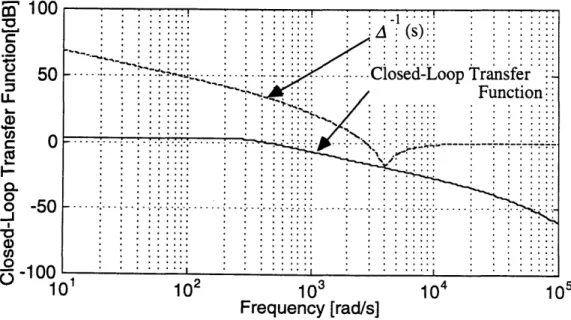
The structure of the controller is the same as that in Figure 2.3. First, the filter gain H is chosen to have the desired characteristics. By tuning the gain of the filter to make the gain of the closed-loop transfer function smaller than A-l(s) and make the sensitivity function close to the one in Figure 2.12, H = [4.66 x 102 1.09 x 105]T . is

chosen. The sensitivity function and the closed-loop transfer function of the filter loop are shown in Figure 2.16 and Figure 2.17. Figure 2.18 and Figure 2.19 are the bode plots of the sensitivity function and closed-loop transfer function of the recovered closed-loop system. Both functions are almost the same as those of the filter's. As a result, we obtain a time response that is similar to but slightly slower than the response in Figure 2.12 (Figure 2.20). The disturbance applied to the system is the same disturbance mentioned in Section 2.3.1, which is the pulse whose amplitude is 50 N and that lasts 2 ms. The stability robustness is also satisfied because the bandwidth of the closed-loop system is properly limited, and as Figure 2.21 shows, even when the sensor dynamics exist, the closed-loop system is stable (However, it shows oscilations because the system is almost on the stable limit).

The problem of the LQR/LTR design is that it is not easy to find the filter gain that realizes the desired filter loop. Moreover, it is difficult to estimate the limitation of the performance we can achieve with the LQG/LTR design procedure. In this example, the limitation of achievable performance was known from the result in the previous section. However, in general case, we might waste a time to select a filter gain by pursuing the impossible performance.

102 103 104

Frequency [rad/s]

Figure 2.16: Sensitivity function of the filter loop.

102 103 104

Frequency [rad/s]

Figure 2.17: Closed-loop transfer function of the filter loop. -5 -10 10

10

Z"-

_Q

10

1A

5r

10 q0 1m o -10 Co -o0 102

10

10

Figure 2.18: Sensitivity function of the LQG/LTR designed system.

102

103

10

Frequency [rad/s]

Figure 2.19: Closed-loop transfer function of the LQG/LTR designed system.

105

oS-50

.I-o

₁₀

t

0.01

0.02

0.03

0.04

Time [sec]

Figure 2.20: Time response of the LQG/LTR designed system.

0.01 0.02 0.03 0.04

Time [sec]

Figure 2.21: Time response of the LQG/LTR designed system with the sensor dy-namics.

2.3.4

p-Synthesis

The H, design and LQG/LTR design can achieve only stability robustness. p-Synthesis has the potential of solving the overall robust control problem including

x 10-

x 10-

0.05

0

0.05

performance robustness. Dyle et al showed performance robustness is expressed in the form of fictitious uncertainties and the small gain theorem [9]. Therefore, the ro-bust control problem can be considered to solve a problem described in Figure 2.22 as a generalized form, and using structure singular values as judging values, we can de-sign a controller that achieves performance robustness as well as stability robustness

[1].

Figure 2.22: Generalized robust control design problem.

In order to demonstrate performance robustness, suppose the case that the mass of the rotor is unknown, but the maximum mass does not exceed 4.5 kg and minimum mass does not become less than 3.0 kg. I try to achieve a sensitivity function lower than the bound described below in Eq.(2.16) no matter how much the mass is within the range from 3.0 kg to 4.5 kg.

10 x 200

s + 200 (2.16)

and D2 in Figure 2.23 as 0 B2 = 4koi2 zo

C2 =

1 0

Then, the system matrices A and B can be written as

0

B

is

the nominal

of the mass of

value

where m, is the nominal value of the mass of

(2.17) (2.18) (2.19)

A2) 0 (2.20)

A2)] (2.21)

the rotor. Then, the corresponding

Figure 2.23: Parametric uncertainty of the system.

nominal mass mn and A2 to m = 3.0 -4.5 kg become the values in Table 2.2.

Figure 2.24 shows the block diagram for this robust performance problem. Once we can describe the problem as this canonical form. we can use the computer aided

Numerical Values

Nominal Mass

Uncertainty

3.6 kg

A 2 5.556 x 10 -2

Table 2.2: Nominal mass and uncertainty.

Figure 2.24: Block diagram of the p-synthesis structure.

design tool to design the controller. p-Synthesis consists of the iteration of an Ho optimal design and curve fitting (D-scale fitting). The design completes when the structured singular values become less than one throughout the all frequencies [1]. Figure 2.25 shows the structured singular value plot before the D-scale fitting has not been done. With the D-scale fitting, I try to minimize the maximum structured singular value and make it less than one. D-scale must be approximated with finite systems. The order of the approximated system should be as low as possible because

eV (Dl o = 10 -i ~J-10 L. 101 102 ₁₀3 ₁₀4 Frequency [rad/s]

Figure 2.25: Structured singular values before D-scale fitting.

the order of the controller becomes huge if we choose a high-order approximation. In this case, a 5th order system is appropriate to approximate the D-scale derived in the process of calculating the structured singular values (Figure 2.26 and Figure 2.27). This D-scale fitting leads the maximum structured singular value of the closed-loop system less than one. How the maximum structured singular value is lowered is shown in Figure 2.28. As seen in Figure 2.28, the structured singular values in the frequency domain become flat (all pass) with the iteration of the Ho optimization and D-scale optimization.

In general case, structured singular values cannot be directly obtained. Only if the number of the blocks, Ai, is less than or equal to three, the structured singular value can be evaluated. Otherwise, we can only evaluate performance robustness by the upper bounds of structured singular values. Yet, the research indicates that even if the number of Ai is more than three, the difference between the upper bound obtained by D-scale fitting and the structured singular value is usually less than 5 %

,. .. . . ... ... - ... ... . .... _ ... . . . .. . .. . . .. ~ .... ... . .

40

20

102

Frequency [rad/s]

10

3

₁₀

Figure 2.26: D-scales and the fitted 5th order curves for A1.

Frequency [rad/s]

Figure 2.27: D-scales and the fitted 5th order curves for A2.

41 * 5th order fit D-scale for A

i

!i

ili

i~

i~

i

,,7,._

i i00

100

-50

-100

1

... ...

..-

..

.

.

.i-i-.

.. ...

20 -10 L. o S-10 C.) L_ . ... .. .... . ...

Before Optimized over D-scales .

101... O1 i 02i D

_ie

,,.,

100 101 102 103 104

Frequency [rad/s]

Figure 2.28: Structured singular values after the D-scale fitting.

[8]. In this case, the number of Ai is two; therefore, the result of the P-synthesis is

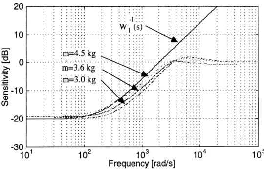
not conservative. Figure 2.29 is the magnitude plot of the sensitivity functions with three different rotor masses. The i-synthesis makes all the sensitivity functions less than the sensitivity bound set as a specification.

2.4

Summary

In this chapter, several controller design methods based on the linear theories were demonstrated. Many of the existing design methods are based on linear theories, and we can choose one of them to achieve the specific purpose such as to minimize the quadratic function of the time response or to guarantee the response time even when uncertainties exist in the system.

In the case of magnetic bearings, stability robustness is essential because of their unstable nature. Moreover, when we use the magnetic bearing for precise

position-tU 20 > 0 Cm C, -20 -An . ..1 .. .I .. . ... .... I .. . ... ... Sensitivity Bound .

-.

.- .. .

-

_.

k

ii

Frequency [rad/s]

Figure 2.29: Sensitivity function with the various rotor masses.

ing, performance robustness is required as well as the stability robustness. For this purpose, M-synthesis is suitable to achieve uniformed responses when uncertainties exist. This robust performance issue is the result of relatively recent researches; thus, there still is an immaturity in the process of design. However, in this chapter, it was demonstrated that the designed system is guaranteed the performance robustness even though conservativeness may exist in some cases.

Table 2.3 shows the comparison among the most often-used linear design meth-ods. As design specifications become complicated, more sophisticated calculations are required. However, most of the design sequences in Table 2.3 are programmed in MATLAB m-files as listed and commercially available. Therefore, all we have to do is to formulate the problems as a canonical form that can fit the computer aided design. The Matlab programs that are used to design the controllers in this chapter are attached in Appendix.

CD3 0 B CI) 0 0 cD '-1~s 0 0 0 cD cD c-0

Features Guarantees Disadvantages MATLAB Commands

* acker (SISO)

Pole Placement - Uses pure gain controller Stability * Need full-state feedback (Control System Toolbox) * Places the closed loop poles * Cannot specify the trade-off - place (MIMO)

(Control System Toolbox)

Eigenstructure * Uses pure gain controller * Need full-state feedback Assignment * Assignes the closed loop poles and - Stability * Cannot specify the trade-off

eigenvectors

LQR Uses a quadratic performance index * Stability margin Need full-state feedback * Iqr

L Uses pure gain controller (gain o, phase 60) Need accurate model (Control System Toolbox) • Possibly many iterations

* Uses a quadratic performance index * Need accurate model • lqr & Iqe

LQG * Uses available noise information in - Stability * No stability margin guaranteed (Control System Toolbox)qg

plant and measurement * Possibly many iterations lqg

(Robust Control Toolbox)

SRecovers High gain controller the target filter loop * ltru

LQG/LTR * Recovers the target filter loop * Robust stability * Minimum phase plant only (Robust Control Toolbox)

* hinf

* Specifies the performance and * Restrictions exist in the form of (Robust Control Toolbox) Hoo robust stability by Hoo norms * Robust stability an augmented plant * hinfsyn

* Exact loop shaping _{(I-Analysis and Synthesis Toolbox)}

* mInusyn

* Uses structured singular values * Robust stability * Problem is nonconvex (Robust Controll Toolbox) -Synthesis Has potential to solve the overall * Robust performance Controller size is huge * dkit

Chapter 3

Limitations of Linear Controllers

3.1

Introduction

In Chapter 2, it was shown that it is possible to design a controller that satisfy the specification with p-synthesis even when uncertainties exist. This performance robustness is especially necessary for the precision magnetic bearings for machining center spindles or the joints of robot manipulators because pay load changes as the machining tool is changed or the configuration of the manipulator changes. We can implement uncertainties in the design specification, and p-synthesis guarantees the uniformed responses within the specified uncertain range. However, if uncertainties are large, linear controllers may not be able to satisfy the specification. The existence of the linear controller that satisfies the specification when uncertainties exist is of interest because if we cannot achieve the specification with linear controllers, we must consider an alternative method. The H, design method can judge the existence of the controller that satisfies the specification. Since p-synthesis is a combination of the

H,, optimal design and D-scale fitting, it has the potential to judge the limitations

of linear controllers for overall robustness problems.

In this chapter, it is first shown how the limitation of the linear controllers is determined by the Ho, design method. Then, the effect of the range of the uncertainty, which is used in Chapter 2 as a design example is examined. In addition, we try to reveal the limitations by using the structured singular value plot. Finally, the possible adverse aspects are listed and how to avoid these disadvantages is discussed.

3.2

Achievable Performance with Limited

Band-width

The H, optimal design method is known to shape the closed-loop transfer function (or sensitivity function) exactly the same shape we plan to be as a shape of the weighting functions. In addition, it gives us the information about the existence of the controller that satisfies the specification given as a shape of weighting functions within the linear frame. For example, consider the case to design a controller for the magnetic bearing that has the parameters shown in Table 2.1. Suppose the sensitivity bound (performance specification) Wi(s) is given as

10 x 200

Wi(s) = (3.1)

s + 200

and the bandwidth of the closed-loop system and the roll-off at the high frequencies are defined as

82

W2(s) = S (3.2)

The performance bound is set to achieve the settling time of about 1 ms and reasonably-small steady state error. The parameter wc is decided by the unmodeled dynamics that exist in the high frequency region as shown in Chapter 2. The stability must be maintained; therefore, the closed-loop transfer function of the designed system must have lower gain than W2-(s) in Eq.(3.2). Thus, the design is proceeded to make the

H,-norm of the closed-loop system

= W_{1(s) (s)}

(3.3)

W2(s)T (s)

less than one, where S(s) is the sensitivity function and T(s) is the closed-loop transfer function. If y exists such that y > 1 and J < 1, the controller that satisfies the specification exists. However, if it does not exist, we have to revise the specification.

The socalled yiteration automatically changes the 7y and evaluates the maximum -that leads J < 1. The maximum singular values of the transfer function from w to z

T(s)

=[

W2(s)T(s)

_(3.4)

of the system designed by -y-iteration are plotted in Figure 3.1 with several ýc. From this figure, we can observe that the limitation of a linear controller that satisfies the performance specification, Eq.(3.1), is somewhere between wu = 3000 rad/s and

wC = 4000 rad/s. In this calculation, the tolerance of y is set to 0.001. The reason why the maximum singular values of Tw, at the high frequencies rolls off is that the optimization is not perfectly done. If a tighter tolerance is chosen, the maximum singular values of Tw, become flat for all frequencies. However, that is not necessary because the tolerance of 0.001 covers all the necessary frequencies.

-5 -1 10 me = 2000 0 c.= 3000

0

::: 4000

Frequency

[rad/s]

Figure 3.1: Maximum singular values of T., (s).

_ __ _~___~ i I I I--U T ·-· •.< - - . .... .. . ' N ,: ...

....

This limitation forces us to revise the performance specification. Figure 3.2 shows the achievable performances with several bandwidth limits wc, and the corresponding closed-loop transfer functions are shown in Figure 3.3.

This feature, to judge the existence of the controller, of the H, design method is powerful because it reveals the limitation of linear controllers with bandwidth limit.

3.3

Limitation with Parameter Uncertainties

In Chapter 2, I showed that we can judge performance robustness by structured singular values. Even though there still is a room to improve, p-synthesis gives us an insight of the limitation of linear controllers when we try to achieve performance robustness. Consider the case given in Section 2.3.4. A controller that satisfies the performance specification even when the mass of the rotor changes at the range of 3.0 to 4.5 kg was designed. Here, how wide range the linear controller can tolerate is of interest because if there are no linear controllers that can achieve the performance robustness, we have to consider other approaches.

Figure 3.4 shows the structured singular value plot of the closed-loop system designed by p-synthesis with various uncertainties. As can be seen from the figure, we can design the controller that satisfies the performance bound, Eq.(3.1), even if the mass of the rotor is unknown but within the range of 3.0 to 4.5 kg. Figure 3.5 shows 10-pm step responses of the closed-loop system with the cases of m = 3.0 kg, m = 3.6 kg (nominal mass), and m = 4.5 kg. Even though the mass increases

50 %, the shapes of the responses are uniformed, and the settling time keeps 1 ms for all three cases. However, if the upper bound of the uncertainty exceeds 4.5 kg, the maximum structured singular value becomes more than one. That means the designed system does not satisfy the specification for the specified uncertainty range.

20 10 -10 -20 30~f 101 102 103

Frequency [rad/s]

10

Figure 3.2: Achievable sensitivity functions with various we.

.:.. . i- c , ("eC ,... ... ... . .... . ... .. =4000 rad/s =

3000

"

o00

rad/s

Frequency [rad/s]

10

Figure 3.3: Closed-loop transfer function of the systems.

49 -7 -· - *: ! : : : ::: :: ._{.. . ...} : : : : : :: .::: _{: :"}: : :. .c = 2000 rad/s co c 3000 rad/s ... o = 4000 rad/s

..

105

-6

100

₁₀

... ·...

-m=3.0-5.0kg

M 0

m=3.0-3.5kg

m=3.

.

4. k

Cn

Frequency [rad/s]

Figure 3.4: Structured singular values with various uncertainty ranges.

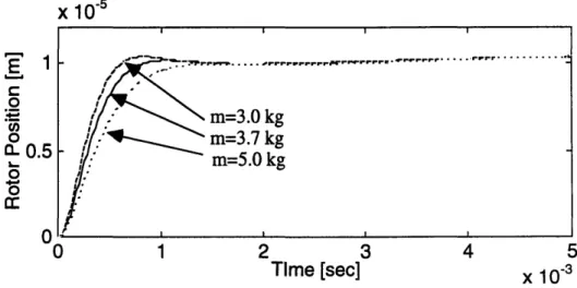
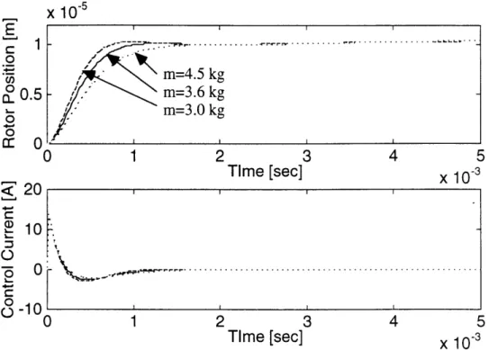
Therefore, if the uncertainty range of the mass is 3 to 5 kg, the resultant sensitivity function by p-synthesis does not become less than W- (s) for all frequencies (Figure 3.6). As a result, in the 10-iLm step response, the shape of the response can have overshoot, or the settling time can take more than 1 ms (Figure 3.7).

When looking into Figure 3.4, we observe that the structured singular values are not flat for all the frequencies. That means the design is not perfectly optimized in terms of lowering the maximum structured singular value. The limitation of linear controllers is precisely estimated when we can obtain an all-pass structured singular values. However, it requires more precise (higher order) approximation for D-scale fitting and smaller tolerance for H. optimization in the p-synthesis process. In this case, a 5th-order approximation for D-scale fitting and a tolerance of 0.01 for

o

x

10-

Time

[sec]

Figure 3.5: Step responses of the system designed for m = 3.0 - 4.5 kg with various

m.

7-iteration are used, and limitations are reasonably estimated.

3.4

Adverse Aspects of Large Uncertainties

It is easily imagined that the robust controller designed by P-synthesis achieves the performance robustness by making the loop gain high. High gain is inevitable within the linear frame to make the system robust. However, high gain causes three adverse effects: high control input, noise magnification, and instability due to unmodeled dynamics. High control input may cause actuator saturation.

It is also imagined that the larger uncertainties the plant has, the higher gain the controller has. Figure 3.8 shows the gain plot of the controller designed by three p-synthesis cases: ma = 0.5 kg, ma = 1.0 kg, and ma = 1.5 kg for

m = 3.0 + mA (kg) (3.5)

As expected, the gain becomes higher when the uncertainty becomes larger. It is also said that the increase of the gain is not proportional to the increase of the uncertainty;

-10 -15

-9

10

Figure 3.6: Sensitivity functions designed for m = 3.0 - 5.0 kg with various m.

x

10-1 2 3 4

Time [sec]

_{x 10-3}

Figure 3.7: Step responses of the system designed for m = 3.0 , 5.0 kg with various

m. lE o S0.5 o 0w

the gain plots of the controller designed for mA = 0.5 kg and mA = 1.0 kg are almost the same shape whereas the gain of the controller designed for mA = 1.5 kg is more than 20 dB higher than the other two cases in high frequencies. This fact is more

130 120 ~' 110 CD 100 90 100 102 104 Frequency [rad/s] 106

Figure 3.8: Gain plot of the controller designed by p-synthesis.

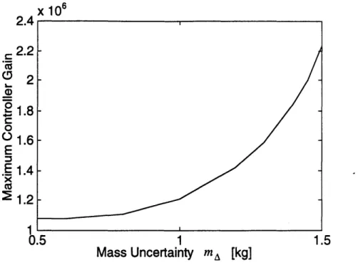
clearly shown in Figure 3.9 that shows how high the maximum gain (H, norm of the controller) becomes when mA increases. As it was mentioned in the previous section, if the uncertainty of the mass exceeds 4.5 kg (ma becomes more than 1.5 kg), the controller that satisfies the specification does not exist. However, even though the controller exists at mA < 1.5 kg, the gain of the controller becomes significantly higher when mA becomes close to the limitation, especially in the high frequency region.

The effect of this high gain can be seen in the control input of step responses. Figure 3.10, 3.11, and 3.12 respectively show the 10-pm step responses of the system

x 106

2.2

o

1.6

E

.E

1.4

Mass Uncertainty

mA

[kg]

Figure 3.9: Increase of the maximum controller gain with the increase of the mass uncertainty.

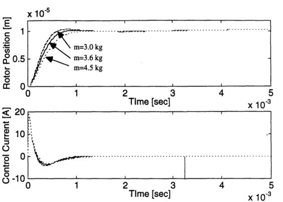
designed for m = 3.0 - 3.5 kg, m = 3.0 , 4.0 kg, and m = 3.0 - 4.5 kg. The systems designed for m = 3.0 - 3.5 kg and m = 3.0 - 4.0 kg show the slow responses at

m = 4.5 kg. However, the control input in both cases does not exceed 10 A whereas in the system designed for m = 3.0 - 4.5 kg, the control input almost reaches 20 A.

The reason why the gain is high when the uncertainties become close to the limitation is that in the optimization process, p-synthesis tries to make the gain highest to make the system insensitive for the parameter change as long as it does not violate the stability robustness. If the uncertainties are not close to the limitation, the system satisfies the specification far before the gain becomes as high as possible. Therefore, we should avoid to design the system that is close to the limitation if we try to use linear controllers in order to avoid the adverse effects that high gain controllers cause.

x

10-s

Time [sec]

x 10-

Time

[sec]

_{x 10}

Step response and the control input of the system designed for m =

x 10-

S10

0-0

Time

[sec]

Figure 3.11: Step response and the control input of the system designed for m = 3.0 - 4.0 kg. E 1. . 0.5 L-o n-" 0 0 20 10 o I-O 0-rt-10 I~~ I V w E U