HAL Id: lirmm-00652293
https://hal-lirmm.ccsd.cnrs.fr/lirmm-00652293
Submitted on 20 Dec 2011
HAL is a multi-disciplinary open access
archive for the deposit and dissemination of
sci-entific research documents, whether they are
pub-lished or not. The documents may come from
teaching and research institutions in France or
abroad, or from public or private research centers.
L’archive ouverte pluridisciplinaire HAL, est
destinée au dépôt et à la diffusion de documents
scientifiques de niveau recherche, publiés ou non,
émanant des établissements d’enseignement et de
recherche français ou étrangers, des laboratoires
publics ou privés.
Efficient Evaluation of SUM Queries Over Probabilistic
Data
Reza Akbarinia, Patrick Valduriez, Guillaume Verger
To cite this version:
Reza Akbarinia, Patrick Valduriez, Guillaume Verger. Efficient Evaluation of SUM Queries Over
Probabilistic Data. IEEE Transactions on Knowledge and Data Engineering, Institute of Electrical
and Electronics Engineers, 2013, 25 (4), pp.764-775. �lirmm-00652293�
1
Efficient Evaluation of SUM Queries over
Probabilistic Data
*
Reza Akbarinia
1, Patrick Valduriez
1, Guillaume Verger
2INRIA and LIRMM, Montpellier, France
1
[email protected], [email protected]
Abstract— SUM queries are crucial for many applications that need to deal with uncertain data. In this paper, we are interested in the
queries, called ALL_SUM, that return all possible sum values and their probabilities. In general, there is no efficient solution for the problem of evaluating ALL_SUM queries. But, for many practical applications, where aggregate values are small integers or real numbers with small precision, it is possible to develop efficient solutions. In this paper, based on a recursive approach, we propose a new solution for this problem. We implemented our solution and conducted an extensive experimental evaluation over synthetic and real-world data sets; the results show its effectiveness.
Index Terms— Database Management, Systems, Query processing.
—————————— ——————————
1
I
NTRODUCTIONAggregate (or aggr for short) queries, in particular SUM queries, are crucial for many applications that need to deal with uncertain data [14] [20] [28]. Let us give two motivating examples from the medical and environ-mental domains.
Example 1: Reducing the usage of pesticides. Consider a plant monitoring application on which we are working with scientists in the field of agronomy. The objective is to observe the development of diseases and insect attacks in the agricultural farms by using sensors, aiming at using pesticides only when necessary. Sensors periodically send to a central system their data about different measures such as the plants contamination level (an integer in [0..10]), temperature, moisture level, etc. However, the data sent by sensors are not 100% certain. The main rea-sons for the uncertainty are the effect of climate events on sensors, e.g. rain, unreliability of the data transmission media, etc. The people from the field of agronomy with which we had discussions use some rules to define a de-gree of certainty for each received data. A decision sup-port system will analyze the sent data, and trigger a pesti-cide treatment when the sum of contamination since the last treatment is higher than a threshold with a high probability. An important query for the decision support system is “given a contamination threshold s, what is the cumulative probability that the contamination sum be higher than s?”. The treatment starts when the query result is higher than a predefined probability.
Example 2: Remote health monitoring. As another ex-ample, we can mention a medical center that monitors key biological parameters of remote patients at their
* Work partially sponsored by the DataRing project of the Agence
Nationale de la Recherche.
Possible Worlds Prob. SUM
w1={t1,t2,t3} 0.16 3 w2={t1,t2} 0.16 1 w3={t1,t3} 0.24 3 w4={t2,t3} 0.04 2 w5={t1} 0.24 1 w6={t2} 0.04 0 w7={t3} 0.06 2 w8={} 0.06 0
Figure 2. The possible worlds and the results of SUM
query in each world, for the database of Figure 1.
Figure 3. Cumulative distribution function for the SUM
query results over the database shown in Figure 1. Tuple Patient Required
nurses … Probability t1 PID1 1 … 0.8 t2 PID2 0 … 0.4 t3 PID3 2 … 0.5
homes, e.g. using sensors in their bodies. The sensors periodically send to the center the patients’ health data, e.g. blood pressure, hydration levels, thermal signals, etc. For high availability, there are two or more sensors for each biological parameter. However, the data sent by sensors are uncertain, and the sensors that monitor the same parameter may send inconsistent values. There are approaches to estimate a confidence value for the data sent by each sensor, e.g. based on their precision [15]. According to the data sent by the sensors, the medical application computes the number of required human resources, e.g. nurses, and equipments for each patient. Figure 1 shows an example table of this application. The table shows the number of required nurses for each pa-tient. This system needs to have sufficient human re-sources in order to assure its services with a high prob-ability. One important query for the system is “given a threshold s, return the cumulative probability that the sum of required nurses be at most s”.
Based on the data in Figure 1, we show in Figure 2 the possible worlds, i.e. the possible database instances, their probabilities, and the result of the SUM query in each world. In this example, there are 8 possible worlds and four possible sum values, i.e. 0 to 3.
In this paper, we are interested in the queries that re-turn all possible sum values and their probabilities. This kind of query, which we call ALL_SUM, is also known as sum probability distribution. For instance, the result of ALL_SUM (required nurses) for the database shown in Figure 1 is {(3, 0.40), (2, 0.10), (1, 0.40), (0, 0.10)}, i.e. for each possible SUM result, we return the result and the probability of the worlds in which this result appears. For instance, the result sum=3 appears in the worlds w1 and
w3, so its probability is equal to P(w1) + P(w3) = 0.16 + 0.24 = 0.40.
By using the results of ALL_SUM, we can generate the cumulative distribution functions, which are important for many domains, e.g. scientific studies. For example to answer the query stated in Erreur ! Argument de commu-tateur inconnu., we need to be able to compute the cumu-lative probability for possible contamination sums that are higher than the threshold s. Similarly, for the query described in Erreur ! Argument de commutateur incon-nu., we should compute the cumulative probability when the sum value is lower than or equal to the threshold. In
Figure 1, by using the results of ALL_SUM, the cumula-tive distribution function of sum values over the data of Figure 1 is depicted.
A naïve algorithm for evaluating ALL_SUM queries is to enumerate all possible worlds, compute sum in each world, and return the possible sum values and their ag-gregated probability. However, this algorithm is expo-nential in the number of uncertain tuples.
In this paper, we deal with ALL_SUM queries and propose pseudo-polynomial algorithms that are efficient in many practical applications, e.g. when the aggr attrib-ute values are small integers or real numbers with small precision, i.e. small number of digits after decimal point. These cases cover many practical aggregate attributes, e.g. temperature, blood pressure, needed human resources per patient in medical applications. To our knowledge, this is the first proposal of an efficient solution for return-ing the exact results of ALL_SUM queries.
1.1 Contributions
In this paper, we propose a complete solution to the prob-lem of evaluating SUM queries over probabilistic data: • We first propose a new recursive approach for
evalu-ating ALL_SUM queries, where we compute the sum probabilities in a database based on the probabilities in smaller databases.
• Based on this recursive approach, we propose a pseudo-polynomial algorithm, called DP_PSUM that efficiently evaluates ALL_SUM queries for the appli-cations where the aggr attribute values are small inte-gers or real numbers with small precision. For exam-ple, in the case of positive integer aggr values, the exe-cution time of DP_PSUM is O(n2×avg) where n is the number of tuples and avg is the average of the aggr values.
• Based on this recursive approach, we propose an algo-rithm, called Q_PSUM, which is polynomial in the number of SUM results.
• We validated our algorithms through implementation over synthetic and real-world data sets; the results show the effectiveness of our solution.
The rest of the paper is organized as follows. In Section 2, we present the probabilistic data models, which we consider and define formally the problem we address. In Sections 3 and 4, we describe our Q_PSUM and DP_PSUM algorithms for evaluating ALL_SUM queries under a simple and frequently used model. In Sections 5 and 6, we extend our solution for a more complex model with some correlations. We also extend our solution for evaluating COUNT queries in Section 6. In Section 7, we report on our experimental validation over synthetic and real-world data sets. Section 8 discusses related work. Section 9 concludes and gives some directions for future work.
2
P
ROBLEMD
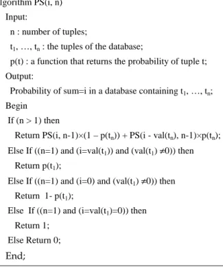
EFINITIONIn this section, we first introduce the probabilistic data Tuple Probability
t1 p1
t2 p2
… …
(a)
Tuple Possible values of aggr attribute, and their probabilities
t1 (v1,1, p1,1), (v1,2, p1,2), …, (v1,m1, p1,m1) t2 (v2,1, p2,1), (v2,2, p2,2), …, (v2, m2, p2,m2)
… …
(b)
Figure 4. Probabilistic data models; a) Tuple-level; b) Attribute-level model
3
models that we consider. Then, we formally define the problem that we address.
2.1 Probabilistic Models
The two main models, which are frequently used in our community, are the tuple-level and attribute-level models [9]. These models, which we consider in this paper, are defined as follows.
Tuple-level model. In this model, each uncertain table T has an attribute that indicates the membership probability (also called existence probability) of each tuple in T, i.e. the probability that the tuple appears in a possible world. In this paper, the membership probability of a tuple ti is denoted by p(ti). Thus, the probability that ti does not appear in a random possible world is 1- p(ti). The data-base shown in Figure 4.a is under tuple-level model.
Attribute-level model. In this model, each uncertain tuple ti has at least one uncertain attribute, e.g. α, and the value of α in ti is chosen by a random variable X. We as-sume that X has a discrete probability density function (pdf). This is a realistic assumption for many applications [9], e.g. sensor readings [12] [22]. The values of α in ti are m values vi,1, …, vi,m with probabilities pi,1, …, pi,m respec-tively (see Figure 4.b). Note that for each tuple we may have a different pdf.
The tuples of the database may be independent or cor-related. In this paper, we first present our algorithms for databases in which tuples are independent. We extend our algorithms for correlated databases in Section 6.1.
2.2 Problem Definition
ALL_SUM query is defined as follows.
Definition 1: ALL_SUM query. It returns all possible sum results together with their probability. In other words, for each possible sum value, ALL_SUM returns the cumulative probability of the worlds where the value appears as a result of the query.
Let us now formally define ALL_SUM queries. Let D be a given uncertain database, W the set of its possible worlds, and P(w) the probability of a possible world
w∈W. Let Q be a given aggr query, f the aggr function stated in Q (i.e. SUM), f(w) the result of executing Q in a world w∈W, and VD,f the set of all possible results of exe-cuting Q over D, i.e. VD,f = {v∃w∈W ∧ f(w)=v}. The cumu-lative probability of having a value v as the result of Q over D, denoted as P(v, Q, D), is computed as follows:
P(v,Q,D)= P(w) w∈W and f (w )=v
∑
Our objective in this paper is to return the results of ALL_SUM as follows:
ALL_SUM (Q, D) = {(v, p) v∈VD,f∧ p= P(v, Q, D)}
3
ALL_SUM
UNDERT
UPLE-
LEVELM
ODELIn this section, we propose an efficient solution for evalu-ating ALL_SUM queries. We first propose a new recur-sive approach for computing the results of ALL_SUM. Then, using the recursive approach we propose our Q_PSUM algorithm.
We assume that the database is under the tuple-level model defined in the previous section. Our solution is extended for the attribute-level model in Section 5. We adapt our solution to process COUNT queries in Section 6.3.
3.1 Recursive Approach
We develop a recursive approach that produces the re-sults of ALL_SUM queries in a database with n tuples based on the results in a database with n-1 tuples. The principle behind it is that the possible worlds of the data-base with n tuples can be constructed by adding / not adding the nth tuple to the possible worlds of the data-base with n-1 tuples.
Let DBn be a database involving the tuples t
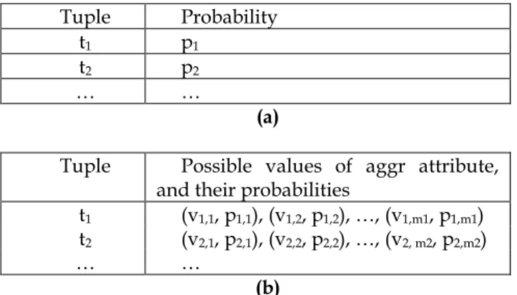
1, …, tn, and ps(i,n) be the probability of having sum = i in DBn, We develop a recursive approach for computing ps(i, n). SUM values and their probabilities in
DBn-1, i.e. a db containing tuples t1, …, tn-1 : 0 : ps(0, n-1) 1 : ps(1, n-1) … i : ps(i, n-1) … DBn-1 0 : ps(0, n-1) × (1 - p(tn)) 1 : ps(1, n-1) × (1 - p(tn)) … i : ps(i, n-1) × (1 - p(tn)) … 0 : 0 … val(tn) – 1 : 0 val(tn) : ps(0, n-1) × p(tn)
i : ps(i - val(tn), n-1) × p(tn), if i≥ val(tn) …
SUM values and their probabilities in DBn DBn
In W1n, i.e. worlds not containing
In W2n, i.e. worlds containing tn Add tuple
tn to the db
Figure 5. Recursively computing the probabilities of SUM
values by adding the nth tuple, i.e. tn, to a db containing n-1 tuples, i.e. DBn-1. The function ps(i, n) denotes the probabil-ity of having sum = i in DBn. The value val(tn) is the aggr value of tuple tn.
3.1.1 Base
Let us first consider the recursion base. Consider DB1, i.e. the database that involves only tuple t1. Let p(t1) be the probability of t1, and val(t1) be the value of t1 in aggr at-tribute. In DB1, there are two worlds: 1) w1={}, in which t1 does not exist, so its probability is (1- p(t1)); 2) w2={t1}, in which t1 exists, so the probability is p(t1). In w1, we have
sum=0, and in w2 we have sum=val(t1). If val(t1) = 0, then we always have sum=0 because in both w1 and w2, sum is zero. Thus, in DB1, ps(i, 1) can be written as follows:
ps (i,1)=
p ( t1) if i=val ( t1) and val ( t1)≠0
1− p ( t1) if i=0 and val ( t1)≠0 1 if i=val ( t1)=0 (1) 0 otherwise 3.1.2 Recursion Step
Now consider DBn-1 , i.e. a database involving the tuples t1, …, tn-1. Let Wn-1 be the set of possible worlds in DBn-1.
We construct DBn by adding tn to DBn-1. Notice that the set of possible worlds in DBn, denoted by Wn, is con-structed by adding / not adding the tuple tn to each world of Wn-1. Thus, in Wn, there are two types of worlds (see Figure 5): 1) the worlds that do not contain tn, de
noted as Wn1; 2) the worlds that contain tn, denoted as Wn2.
For each world w∈ Wn1, we have the same world in DBn-1,say w'. Let p(w) and p(w') be the probability of worlds w and w'. The probability of w, i.e. p(w), is equal to p(w')×(1 – p(tn)), because tn does not exist in w even though it is involved in the database. Thus, in Wn
1 the
sum values are the same as in DBn-1, but the probability of sum=i in Wn1 is equal to the probability of having sum=i in DBn-1 multiplied by the probability of non-existence of tn. In other words, we have:
In Wn1: (probability of sum=i) = ps(i, n-1)×(1 – p(tn)) (2)
Let us now consider Wn
2. The worlds involved in Wn2 are constructed by adding tn to each world of DBn-1. Thus, for each sum value equal to i in DBn-1 we have a sum value equal to (i + val(tn)) in Wn2, where val(tn) is the value of aggr attribute in tn. Therefore, the probability of sum= i
+ val(tn) in Wn2 is equal to the probability of sum=i in DBn-1 multiplied by the existence probability of tn. In other words, we have:
In Wn2: (probability of sum=i) = ps(i - val(tn), n-1)×p(tn) (3)
The probability of sum=i in DBn is equal to the prob-ability of sum=i in Wn1 plus the probability of sum=i in Wn
2. Thus, using the Equations 2 and 3, and using the base of the recursion, i.e. Equation 1, we obtain the fol-lowing recursive formula for the probability of sum=i in DBn, i.e. ps(i, n) :
ps(i,n)=
ps(i,n−1)×(1−p(tn))+ps(i−val(tn), n−1)×p(tn) if n>1 1−p(t1) if n=1 and i=0 and val(t1)≠0
p(t1) if n=1 and i=val(t1) and val(t1)≠0
1 if n=1 and i=val(t1)=0 (4) 0 otherwise
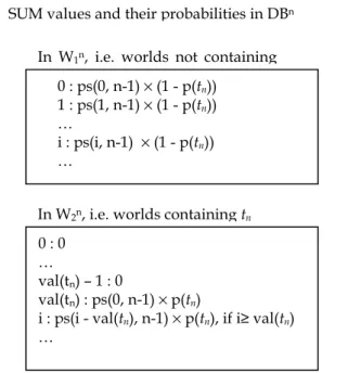
Based on the above recursive formula, we can develop a recursive algorithm for computing the probability of sum=i in a database containing tuples t1, …, tn (see the pseudocode in Figure 6). However, the execution time of the algorithm is exponential in the number of uncertain tuples, i.e. due to the two recursive calls in the body of the algorithm.
3.2 Q_PSUM Algorithm
In this section, based on our recursive definition, we pro-pose an algorithm, called Q_PSUM, whose execution time is O(n × N) where n is the number of uncertain data, and N is the number of distinct sum values.
Q_PSUM uses a list for maintaining the computed pos-sible sum values and their probabilities. It fills the list by starting with DB1, i.e. a database containing only t1, and then it gradually adds other tuples to the database and updates the list.
Let Q be a list of pairs (i, ps) such that i is a possible sum value and ps its probability. The Q_PSUM algorithm proceeds as follows (see the pseudocode in Appendix C). It first initializes Q for DB1 by using the base of the recur-sive definition. If val(t1) = 0, then it inserts (0, 1) into Q, else it inserts (0, 1 - p(t1)) and (val(t1), p(t1)). By inserting a pair to a list, we mean adding the pair to the end of the list.
Then, in a loop, for j=2 to n, the algorithm adds the tu-ples t2 to tn to the database one by one, and updates the list by using two temporary lists Q1 and Q2 as follows. For
Algorithm PS(i, n) Input:
n : number of tuples;
t1, …, tn : the tuples of the database;
p(t) : a function that returns the probability of tuple t; Output:
Probability of sum=i in a database containing t1, …, tn;
Begin If (n > 1) then
Return PS(i, n-1)×(1 – p(tn)) + PS(i - val(tn), n-1)×p(tn);
Else If ((n=1) and (i=val(t1)) and (val(t1) ≠0)) then
Return p(t1);
Else If ((n=1) and (i=0) and (val(t1) ≠0)) then
Return 1- p(t1);
Else If ((n=1) and (i=val(t1)=0)) then
Return 1; Else Return 0;
End;
Figure 6. Recursive algorithm for computing the probability of sum=i in a database containing t1, …,
5
each tuple tj, Q_PSUM removes the pairs involved in Q one by one from the head of the list, and for each pair (i, ps)∈Q, it inserts (i, ps×(1 – p(tj)) into Q1 and (i+val(tj),
ps×p(tj)) into Q2. Then, it merges the pairs involved in Q1 and Q2, and inserts the merged results into Q.
The merging is done on the sum values of the pairs. That means that for each pair (i, ps1)∈Q1 if there is a pair
(i, ps2) ∈Q2, i.e. with the same sum value, then Q_PSUM removes the pairs from Q1 and Q2 and inserts (i, ps1 + ps2) into Q. If there is (i, ps1)∈Q1 but there is no pair (i, ps2) ∈Q2, then it simply removes the pair from Q1 and inserts it to Q.
Let us now analyze the complexity of Q_PSUM. Let N be the number of possible (distinct) sum results. Suppose the lists are implemented using a structure such as linked list (with pointers to the head and tail of the list). The cost of inserting a pair to the list is O(1), and merging two lists is done in O(N)1. For each tuple, at most N pairs are in-serted to the lists Q1 and Q2, and this is done in O(N). The merging is done in O(N). There are n tuples in the data-base, thus the algorithm is executed in O(n × N). The space complexity of the algorithm is O(N), i.e. the space needed for the lists.
4
DP_PSUM
A
LGORITHMIn this section, using the dynamic programming tech-nique, we propose an efficient algorithm, called DP_PSUM, designed for the applications where aggr values are integer or real numbers with small precisions. It is usually much more efficient than the Q_PSUM algo-rithm (as shown by the performance evaluation results in Section 4.5).
Let us assume, for the moment, that the values of aggr attribute are positive integer numbers. In Section 4.3, we adapt our algorithm for real numbers with small preci-sions, and in Section 4.4, we deal with negative integer numbers.
4.1 Basic Algorithm
Let MaxSum be the maximum possible sum value, e.g. for positive aggr values MaxSum is the sum of all values. DP_PSUM uses a 2D matrix, say PS, with (MaxSum + 1) rows and n columns. DP_PSUM is executed on PS, and when it ends, each entry PS[i, j] contains the probability of sum=i in a database involving tuples t1, …, tj.
DP_PSUM proceeds in two steps as follows (the pseu-docode is shown in Appendix C). In the first step, it ini-tializes the first column of the matrix. This column repre-sents the probability of sum values for a database involv-ing only the tuple t1. DP_PSUM initializes this column using the base of our recursive formula (described in Equation 1) as follows. If val(t1) = 0, then PS[0, 1] = 1. Otherwise, PS[0, 1] = (1 – p(t1)) and PS[val(t1), 1] = p(t1). The other entries of the first column should be set to zero, i.e. PS[i, 1] = 0 if i≠0 and i≠val(t1).
In the second step, in a loop, DP_PSUM sets the values
1 Notice that the pairs involved in Q1 and Q2 are systematically ordered
according to sum values, because they follow the same order as the values in Q which is initially sorted.
of each column j (for j=2 to n) by using our recursive definition (i.e. Equation 4) and based on the values in column j-1 as follows:
PS[i, j] = PS[i, j-1]×(1 – p(tj)) + PS[i – val(tj), j-1] ×p(tj) Notice that if (i < val(tj)), then for the positive aggr values we have PS[i – val(tj), j-1]=0, i.e. because there is no possible sum value lower than zero. This is why, in the algorithm only if (i ≥ val(tj)), we consider PS[i – val(tj), j-1]
×p(tj) for computing PS[i, j].
Theorem 1. DP_PSUM works correctly if the database is under the tuple-level model, and the aggr attribute values are positive integers, and their sum is less than or equal to MaxSum.
Proof. Implied by using the recursive formula in Equa-tion 4. □
Let us now illustrate DB_PSUM using the following example.
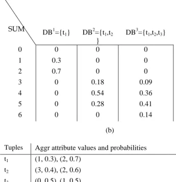
Example 3. Figure 7.b shows the execution of DP_PSUM over the database shown in Figure 7.a. In the first column, we set the probability of sum values for DB1, i.e. a database that only involves t1. Since the aggr value of t1 is equal to 1 (see Figure 7.a), in DB1 there are two possible sum values, sum=1 and sum=0 with probabilities 0.3 and (1 – 0.3) = 0.7 respectively. The probabilities in other columns, i.e. in 2nd and 3rd, are computed using our recursive definition. After the execution of the algorithm, the 3rd column involves the probability of sum values in the entire database. If we compute ALL_SUM by enu-merating the possible worlds, we obtain the same results.
4.2 Complexity
Let us now discuss the complexity of DP_PSUM. The first step of DP_PSUM is done in O(MaxSum), and its second step in O(n×MaxSum). Thus, the time complexity of DP_PSUM is O(n×MaxSum), where n is the number of uncertain tuples and MaxSum the sum of the aggr values of all tuples. Let avg be the average value of aggr values of tuples, then we have MaxSum = n×avg. Thus, the com-plexity of DP_PSUM is O(n2×avg) where avg is the aver-age of the aggr values in the database.
Notice that if avg is a small number compared to n, then DP_PSUM is done in a time quadratic to the input. But, if avg is exponential in n, then the execution time becomes exponential. Therefore, DP_PSUM is a pseudo polynomial algorithm.
The space requirement of DP_PSUM is equivalent to a matrix of (MaxSum + 1) × n, thus the space complexity is O(n2×avg). In Section 4.2.1, we reduce the space complex-ity of DP_ PSUM to O(n×avg).
4.2.1 Reducing space complexity
In the basic algorithm of DP_PSUM, for computing each column of the matrix, we use only the data that are in the precedent column. This observation gave us the idea of using two arrays instead of a matrix for comput-ing ALL_SUM results as follows. We use two arrays of size (MaxSum + 1), e.g. ar1 and ar2. First, we initialize ar1 using the recursion base (like the first step of the basic version). Then, for i =2, …, n steps, DP_PSUM fills ar2 using the probabilities in ar1, based on the recursion step, then it copies the data of ar2 into ar1, and starts the next
step. Instead of copying the data from ar2 into ar1, we can simply change the pointers of ar1 to that of ar2, and renew the memory of ar2.
The space requirement of this version of DP_PSUM is O(MaxSum) which is equivalent to O(n×avg) where avg is the average value of aggr values.
4.3 Supporting real attribute values with small precisions
In many applications that work with real numbers, the precision of values, i.e. the number of digits after decimal point, is small. For example, in medical applications the temperature of patients requires real values with one digit of precision. DP_PSUM can be adapted to work for those applications as follows. Let DB be the input data-base, and c be the number of precision digits in the aggr values. We generate a new database DB' as follows. For each tuple t in the input database DB, we insert a tuple t' to DB' such that the aggr value of t', say v', is equal to the aggr value of t, say v, multiplied by 10c, i.e. v' = v×10c. Now, we are sure that the aggr values in DB' are integer, and we can apply the DP_PSUM algorithm on it. Then, for each ALL_SUM result (v'i, p) over DB', we return (v'i
/10c, p) as a result of ALL_SUM in DB.
The correctness of the above solution can be implied by the fact that, if we multiply all aggr values of a DB by a constant k, then every possible sum result is multiplied by k.
The time complexity of this version of DP_PSUM for aggr attribute values with c digits of precision is O(n×MaxSum×10c) which is equivalent to O(n2×avg×10c) where avg is the average of the aggr attribute values. The space complexity is O(n×avg×10c).
4.4 Dealing with negative integer values
The basic version of DP_PSUM assumes integer values that are positive, i.e. ≥ 0. This assumption can be relaxed as follows. Let MinNeg be the sum of all negative aggr values. Then, the possible sum values are integer values in [MinNeg … MaxSum] where MaxSum is the maximum possible sum value, i.e. the sum of positive aggr values. Thus, to support negative values, the size of the first di-mension of the matrix should be modified to (MaxSum + 1 + MinNeg). In addition, the algorithm should scan the possible sum values from MinNeg to MaxSum, instead of 0 to MaxSum. Morever, since the index in the matrix can-not be negative, we should shift the index of the first dimension by MinNeg.
4.5 Leveraging GCD
For the case of integer aggr values, if the greatest common divisor (GDC) of the values is higher than 1, e.g. when the values are even, then we can significantly improve the performance of the DP_PSUM algorithm as follows. Let DB be the given database, and g be the GCD of the aggr values. We generate a new database DB' in which the tuples are the same as in DB except that the aggr values are divided by g. Then, we apply DP_PSUM on DB', and for each sum result (v'i, p), we return (v'i × g, p) to the user.
In most cases, the GCD of aggr values is 1, so the above
approach is not applicable. However, when we know that GCD is higher than one, using this approach can reduce the time and space complexities of DP_PSUM by an order of GCD, i.e. since the average of the aggr values in data-base DB' is divided by GCD. For example, if the aggr values in DB are {10, 20, 30}, then in the database DB' the aggr values are {1, 2, 3}, i.e. GCD=10. Since the average of aggr values is reduced by 10, the space and time complex-ity of the DP_SUM algorithm will be reduced by an order of 10.
4.6 Skipping Zero Points
During execution of the basic version of our DP_PSUM algorithm, there are many cells (of the matrix) with zero points, i.e. zero probability values. Obviously, we do not need to read zero points because they cannot contribute to non-zero probability values. We can avoid accessing zero points using the following approach. Let L be a list that is initially set to zero. During the execution of the algorithm we add the index of non zero points to L, and for filling each new column, we take into account only the cells whose indices are in L.
This approach improves significantly the performance of DP_PSUM, in particular when the number of tuples is very small compared to the average of aggr values, i.e. avg. For example, if there are only two tuples and avg is equal to 10, then each column of the matrix has about 20 cells. However, there are at most 6 non-zero cells in the matrix, i.e. 2 in the first and at most 4 in the 2nd. Thus, the above approach allows us to ignore almost 70% of the cells.
5
ALL_SUM
UNDERA
TTRIBUTE-L
EVELM
ODELDue to the significant differences between the tuple-level and the attribute-level models it is not trivial to adapt our yet proposed algorithms for the attribute-level model.
(b)
Figure 7. a) A database example in tuple-level model; b) Execution of DP_PSUM algorithm over these exam-ple Tuples Aggr Attribute Value Membership Probability t1 1 0.3 t2 3 0.4 t3 2 0.5 (a SUM DB 1 ={t1} DB2={t1,t2} DB3={t1,t2,t3} 0 0.7 0.42 0.21 1 0.3 0.18 0.09 2 0 0 0.21 3 0 0.28 0.23 4 0 0.12 0.06 5 0 0 0.14 6 0 0 0.06
7
In this section, we propose our solution for computing ALL_SUM results under the attribute-level model.
5.1 Recursive Approach
We propose a recursive approach for computing ALL_SUM under the attribute-level model. This approach is the basis for a dynamic programming algorithm that we describe next. We assume that all tuples have the same number of possible aggr values, say m. This as-sumption can be easily relaxed as we do in Appendix B. We also assume that, in each tuple ti, the sum of the prob-abilities of possible aggr values is 1, i.e. pi,1 + pi,2 + … + pi,m
= 1. In other words, we assume that there is no null value. However, this assumption can be relaxed as in Appendix A.
5.1.1 Recursion Base
Let us consider DB1, i.e. a database that only involves t1. Let v1,1, v1,2, …, v1,m be the possible values for the aggr attribute of t1, and p1,1, p1,2, …, p1,m their probabilities, re-spectively. In this database, the possible sum values are the possible values of t1. Thus, we have:
ps(i,1)= p1,k if∃k such that v1,k =i
0 otherwise (5) 5.1.2 Recursion Step
Now consider DBn-1, i.e. a database involving the tuples t1, …, tn-1. Let Wn-1 be the set of possible worlds for DBn-1. Let
ps(i, n-1) be the probability of having sum=i in DBn-1, i.e. the aggregated probability of the DBn-1 worlds in which we have sum=i. Let vn,1, .. vn,m be the possible values of tn’s aggr attribute, and pn,1, .. pn,m their probabilities. We con-struct DBn by adding tn to DBn-1. The worlds of DBn are constructed by adding to each w∈ Wn-1, each possible value of tn. Let Wnk ⊆Wn be the set of worlds which are constructed by adding the possible value vn,k of tn to the worlds of Wn-1. Indeed, for each world w∈Wn-1 there is a corresponding world w'∈Wn
k such that w' = w + {tn} where the possible aggr value of tn is equal to vn,k. This implies that for each possible sum=i with probability p in Wn-1, there is a possible sum = i + vn,k with probability p × pn,k in Wnk. Recall that ps(i, n-1) is the aggregate probabil-ity of the DBn-1 worlds in which sum = i. Then we have:
Probability of sum=i in Wnk = ps(i – vn,k, n-1) × pn,k;
for k=1, …, m (6)
Let ps(i, n) be the probability of sum=i in DBn. Since we have Wn = Wn1 ∪ Wn2 ∪ … ∪ Wnm, the probability of sum=i in Wn is equal to the sum of the probabilities of sum=i in Wn1, Wn2, … and Wnm. Thus, using Equation 6 and the recursion base of Equation 5, the probability of sum=i in DBn, i.e. ps(i, n), can be stated as follows:
ps(i, n)=
ps(i−
k=1
m
∑
vn,k, n−1)×pn,k if n>1p1,k if n=1and∃k such that v1,k =i
0 otherwise (7)
5.2 Dynamic Programming Algorithm for Attribute-level Model
Now, we describe a dynamic programming algorithm, called DP_PSUM2, for computing ALL_SUM under the attribute-level model. Here, similar to the basic version of DP_PSUM algorithm, we assume integer values. How-ever, in a way similar to that of DP_PSUM, this assump-tion can be relaxed. Let PS be a 2D matrix with (MaxSum + 1) rows and n columns, where n is the number of tuples and MaxSum is the maximum possible sum, i.e. the sum of the greatest values of aggr attribute in the tuples. At the end of DP_PSUM2 execution, PS[i,j] contains the probability of sum=i in a database involving tuples t1, …,
tj.
DP_PSUM2 works in two steps. In the first step, it ini-tializes the first column of the matrix, by using the base of the recursive definition, as follows. For each possible aggr value of tuple t1, e.g. v1,k, it sets the corresponding entry equal to the probability of the possible value, i.e. it sets P[v1,k, 1]=p1,k for 1≤k≤m.
In the second step, DP_PSUM2 sets the entry values of each column j (for 2≤j≤n) by using the recursion step of the recursive definition, and based on the values yet set in precedent column. Formally, for each column j and row i it sets PS[i, j] = ∑ (PS[i - v1,k, j-1] × pj,k) for 2≤k≤m such that i ≥ v1,k.
Let us now analyze the complexity of the algorithm. Let avg=MaxSum/n, i.e. the average of the aggregate at-tribute values. The space complexity of DP_PSUM2 is exactly the same as that of DP_PSUM, i.e. O(n2×avg). The time complexity of DP_PSUM2 is O(MaxSum×n×m). In other words its time complexity is O(m×n2×avg).
Let us now illustrate the DB_PSUM2 algorithm using (b) SUM DB1 ={t1} DB 2 ={t1,t2 } DB3={t1,t2,t3} 0 0 0 0 1 0.3 0 0 2 0.7 0 0 3 0 0.18 0.09 4 0 0.54 0.36 5 0 0.28 0.41 6 0 0 0.14
Tuples Aggr attribute values and probabilities
t1 (1, 0.3), (2, 0.7)
t2 (3, 0.4), (2, 0.6)
t3 (0, 0.5), (1, 0.5)
(a)
Figure 8. a) A database example in attribute-level model;
b) Execution of DP_PSUM algorithm over these exam-ples
an example.
Example 4. Consider the database in Figure 8.a which is under attribute-level model. The execution of the DP_PSUM2 algorithm is shown in Figure 8.b. The first column of the matrix is filled using the probabilities of the possible aggr values of t1. Thus, we set 0.3 and 0.7 for sum values 1 and 2 respectively. The other columns are filled by using our recursive definition. After the execution of the algorithm, the 3rd column shows the probability of all sum results for our example database.
6
E
XTENSIONSIn this section, we extend our algorithm to deal with the x-relation model, and correlated databases with mutual exclusions. We also show how our ALL_SUM algorithms can be used for computing the results of COUNT aggre-gate queries.
6.1 ALL_SUM in X-Relation Model
In the X-Relation model [1], a probabilistic table is com-posed of a set of independent tuples, such that each x-tuple consists of some mutually exclusive x-tuples, called alternatives. Each alternative is associated with a prob-ability. If every x-tuple consists of only one alternative, then the x-relation is equivalent to our tuple-level model. In this case, ALL_SUM query processing can be done using the algorithms developed for tuple-level model.
Let us deal with the problem of evaluating ALL_SUM queries for the case of multiple alternative x-tuples. This problem can be reduced to a problem in the attribute-level model as follows. Let Q be the ALL_SUM query, and α be the aggr attribute. Let D be the given database in the x-relation model. We convert D to a database D' in the attribute-level model such that the result of the query Q in D’ be the same as that of D. The database D’ is con-structed as follows. For each x-tuple x in D, we create a tuple t' in D' with an attribute α. Let T be the set of x’s alternative tuples. Let T’⊆T be the set of tuples in T that satisfy the Q’s predicates. The values of the attribute α in t’ will be the distinct values of this attribute in the tuples involved in T’, and probability of each value is computed in a similar way as a projection on α. In other words, if a value appears in only one alternative of x, then its prob-ability is equal to the probprob-ability of the alternative. Oth-erwise, i.e. when a value appears in multiple alternatives, its probability is equal to the probability that at least one of the alternatives exists.
Now, the database D' is under the attribute-level model, and we can apply our ALL_SUM algorithms to evaluate ALL_SUM queries over it.
6.2 ALL_SUM over Correlated Databases
In previous sections, we assumed that the tuples of the database are independent. Here, we assume mutual ex-clusion correlations, and show how to execute over ALL_SUM algorithms over databases that contain such correlation. Two tuples t1 and t2 are mutually exclusive, iff they cannot appear together in any instance of the database (i.e. possible world). But, there may be instances in which none of them appear. As an example of mutual exclusive
tuples we can mention the tuples that are produced by two sensors that monitor the same object at the same time. In this example, at most one of the produced tuples can be correct, so they are mutually exclusive.
It has been shown that the tuples of a correlated data-base with mutual exclusions can be grouped to a set of blocks such that there is no dependency between any two tuples that belong to two different blocks, and there are closure dependencies between any two tuples of each block [11]. These blocks are in fact x-tuples with multiple alternatives. Thus, to evaluate ALL_SUM queries on them, it is sufficient to convert the given database to a database D’ in the attribute-level model as shown in Sec-tion 6.1, and then apply an ALL-SUM algorithm that works on the attribute-level model.
6.3 Evaluating ALL_COUNT Queries Using ALL_SUM Algorithms
We now show how we can evaluate ALL_COUNT que-ries, i.e. all possible counts and their probabilities, using the algorithms that we proposed for ALL_SUM. Under the attribute-level model, all tuples are assumed to exist, thus the result of a count query is always equal to the number of tuples that satisfy the query. However, under the tuple-level model, the problem of evaluating ALL_COUNT is harder because there may be (n+1) pos-sible count results (i.e. from 0 to n) with different prob-abilities, where n is the number of uncertain tuples. This is why we deal with ALL_COUNT only under the tuple-level model.
The problem of ALL_COUNT can be reduced to that of ALL_SUM in polynomial time as follows. Let D be the database on which we want to execute ALL_COUNT. We generate a new database D' as follows. For each tuple t∈D we generate a tuple t' in D' such that t' involves only one attribute, e.g. B, with two possible values: v1=1 and
v2=0. We set p(v1) equal to the membership probability of
t. We set p(v2)= 1 – p(v1). Now, if we apply one of our ALL_SUM algorithms over B as aggr attribute in D', the result is equivalent to applying an ALL_COUNT algo-rithm over the aggr attribute in D. This is proven by the following theorem.
Theorem 2. If the database D is under the tuple-level model, then the result of ALL_SUM over the attribute B in database D' is equivalent to the result of ALL_COUNT over the aggregate attrib-ute of the database D.
Proof. If the database D is under the tuple-level model, its membership probability in D is equal to the probabil-ity of value v1=1 in attribute B of D'. Thus, the contribu-tion of a tuple t to COUNT in the database D is equal to the contribution of its corresponding tuple t' to SUM in the database D'. In other words, the results of ALL_SUM over D' is equivalent to the results of ALL_COUNT over D. □
7
E
XPERIMENTALV
ALIDATIONTo validate our algorithms and investigate the impact of different parameters, we conducted a thorough experi-mental evaluation. In Section 7.1, we describe our
ex-9
perimental setup, and in Section 7.2, we report on the results of various experiments to evaluate the perform-ance of the algorithms by varying different parameters.
7.1 Experimental Setup
We implemented our DP_PSUM and Q_PSUM algo-rithms in Java, and we validated them over both real-world and synthetic databases.
As real-world database, like some previous works, e.g. [18] [21], we used the data collected in the International Ice Patrol (IIP) Iceberg Sightings Database (http://nsidc.org/data/g00807.html) whose data is about the iceberg evolution sightings in North America. The database contains attributes such as iceberg, number, sighting date, shape of the iceberg, number of days drifted, etc. There is an attribute that shows the confi-dence level about the source of sighting. In the dataset that we used, i.e. that of 2008, there are 6 confidence lev-els: R/V (radar and visual), VIS (visual only), RAD (radar only), SAT-LOW (low orbit satellite), SAT-MED (medium orbit satellite) and SAT-HIGH (high orbit satellite). Like in [18] and [21], we quantified these confidence levels by 0.8, 0.7, 0.6, 0.5, 0.4 and 0.3 respectively. As aggr attribute, we used the number of drifted days that contains real
numbers with one digit of precision in the interval of [0… 365].
As synthetic data, we generated databases under the attribute-level model that is more complete than the tu-ple-level model. We generated two types of databases, Uniform and Gaussian, in which the values of attributes in tuples are generated using a random generator with the uniform and Gaussian distributions, respectively. The default database is Uniform, and the mean (average) of the generated values is 10. Unless otherwise specified, for the Gaussian database the variance is half of the mean. The default number of attribute values in each tuple of our attribute-value model is 2.
In the experiments, we evaluated the performance of our DP_PSUM and Q_PSUM algorithms. We also com-pared their performance with that of the naïve algorithm that enumerates the possible worlds, computes the sum in each world, and returns the possible sum values and the aggregated probability of the worlds where they appear as the result of sum. To manage the possible sum values, we used a B-tree structure.
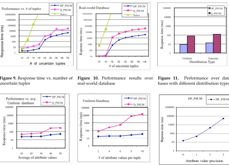
For the three algorithms, we measured their response time. We conducted our experiments on a machine with a 2.66 GHz Intel Core 2 Duo processor and 2GB Figure 9. Response time vs. number of
uncertain tuples
Figure 10. Performance results over real-world database
Figure 11. Performance over data-bases with different distribution types
DP_PSUM 1 10 100 1000 10000 100000 0 1 2 3
Attribute value precision
R ep o n se t im e (m s) DP _P SUM
Figure 12. Effect of the average of aggregate attribute values on per-formance
Figure 13. Effect of the number of at-tribute values per tuple on performance
Figure 14. Effect of the precision of real aggr values on performance
memory.
7.2 Performance Results
In this section, we report the results of our experiments. Effect of the number of uncertain tuples. Using the synthetic data, Figure 9 shows the response time of the three algorithms vs. the number of uncertain tuples, i.e. n, and the other experimental parameters set as described in Section 7.1. The best algorithm is DP_PSUM, and the worst is the Naïve algorithm. For n>30, the response time of the Naïve algorithm is too long, such that we had to halt it. This is why we do not show its response time for n>30. The response time of DP_PSUM is at least four times lower than that of Q_PSUM (notice that the figure is in logarithmic scale).
Over the IIP database, Figure 10 shows the response time of the three algorithms, with different samples of the IIP database. In each sample, we picked a set of n tuples, from the first to the nth tuple of the database. Overall, the results are qualitatively in accordance with those over synthetic data. However, the response time over the real database is higher than that of the synthetic database. The main reason is that the precision of the real data is 1, i.e. there is one digit after the decimal point. This increases the execution time of our algorithms significantly. For example, in the case of DP_PSUM, the execution time can increase up to ten times, and this confirms the complexity analysis of real value processing in Section 4.3.
Effect of data distribution. Figure 11 shows the re-sponse time of our algorithms over the Uniform and Gaussian databases. The response time of DP_PSUM over uniform distribution increases, but not significantly, i.e. less than 30%. The higher performance of DP_PSUM over the uniform distribution is due to the higher number of zero points, which can be skipped (see Table 1), thus less computation is needed. Another reason is the value of MaxSum, i.e. the maximum possible sum value, which is lower for the uniform dataset as shown in Table 1.
The impact of the distribution on Q_PSUM is much more significant, i.e. about two times more than on the DP_PSUM. The reason is that the distribution of the at-tribute values affects the number of possible sum results, i.e. with the Gaussian distribution the number of possible sum values is much more than that of the uniform distri-bution.
Effect of average. We performed tests to study the ef-fect of the average of aggregate values in the database, i.e. avg, on performance. Using the synthetic data, Figure 12 shows the response time of our DP_PSUM and Q_PSUM
algorithms with avg increasing up to 50, and the other experimental parameters set as described in Section 7.1. The average of aggregate values has a linear impact on DP_PSUM, and this is in accordance with the complexity analysis done in Section 4. What was not expected is that the impact of avg on the performance of Q_PSUM is sig-nificant, although avg is not a direct parameter in the complexity of Q_PSUM (see Section 3.2). The explanation is that the time complexity of Q_PSUM depends on the number of possible SUM results, and when we increase avg (i.e. mean) of the aggregate values, their range be-come larger, thus the total number of possible sum values increases.
Effect of the number of attribute values per tuple. We tested the effect of the number of attribute values in each tuple under the attribute-level model, i.e. m, on perform-ance. Figure 13 shows the response time of our algorithms with increasing m up to 10, and other parameters set as in Table 1. This number has a slight impact on DP_PSUM, but a more considerable impact on Q_PSUM.
Effect of precision. We studied the effect of the preci-sion of real numbers, i.e. the number of digits after deci-mal point, on the performance of the DP_PSUM algo-rithm. Using the synthetic data, Figure 14 shows the re-sponse time with increasing the precision of the aggr values. As shown, the precision has a significant impact on the response time of DP_PSUM, i.e. about ten times for each precision digit. This is in accordance with our theo-retical analysis done in Section 4, and shows that our algorithm is not appropriate for the applications in which the aggr values are real numbers with many digits after the decimal point.
8
R
ELATEDW
ORKIn the recent years, we have been witnessing much inter-est in uncertain data management in many application areas such as data cleaning [3], sensor networks [12] [21], information extraction [19], etc. Much research effort has been devoted to several aspects of uncertain data man-agement, including data modeling [4] [6] [10] [16] [17] [29], skyline queries [5] [26], top-k queries [9] [13] [18] [30], near-est neighbor search [31] [33] [35], spatial queries [34], XML documents [1] [24] [25], etc.
There has been some work dealing with aggregate query processing over uncertain data. Some of them were devoted to developing efficient algorithms for returning the expected value of aggregate values, e.g. [7] [20]. For example in [20], the authors study the problem of com-puting aggregate operators on probabilistic data in an I/O efficient manner. With the expected value semantics, the evaluation of SUM queries is not very challenging. In [10], Dalvi and Suciu consider both expected value and ALL_SUM, but they only propose an efficient approach for computing the expected value.
Approximate algorithms have been proposed for probabilistic aggregate queries, e.g. [8] and [28]. The Cen-tral Limit theorem [27] can be used to approximately estimate the distribution of sums for sufficiently large numbers of probabilistic values. However, in the current Table 1. The value of MaxSum and the percentage
of zero points during the execution of DP_PSUM algorithm on uniform and Gaussian datasets.
Uniform Gaussian
MaxSum 2577 3123
Rate of zero value cells
11
paper, our objective is to return exact probability values, not approximations.
In [23] and [32], aggregate queries over uncertain data streams have been studied. For example, Kanagal et al. [23] deal with continuous queries over correlated uncer-tain data streams. They assume correlated data which are Markovian and structured in nature. Their probabilistic model and the assumptions, and as a result the possible algorithms, are very different from ours. For example in their model, they propose algorithms that deal with MIN/MAX queries in a time complexity that does not depend on the number of tuples. However, in our model it is not possible to develop algorithms with such a com-plexity.
The work in [11] studies the problem of HAVING ag-gregate queries with predicates. The addressed problem is related to the #KNAPSACK problem which is NP-hard. The difference between HAVING-SUM queries in [11] and our ALL_SUM queries is that in ALL_SUM we return all possible SUM values and their probabilities, but in HAVING-SUM the goal is to check a condition on an aggregate function, e.g. is it possible to have SUM equal to a given value.
Overall, for the problem that we considered in this pa-per, i.e. returning the exact results of ALL_SUM queries, there is no efficient solution in the related work. In this paper, we proposed pseudo polynomial algorithms that allow us to efficiently evaluate ALL_SUM queries in many practical cases, e.g. where the aggregate attribute values are small integers, or real numbers with limited precisions.
9
C
ONCLUSIONSUM aggr queries are critical for many applications that need to deal with uncertain data. In this paper, we ad-dressed the problem of evaluating ALL_SUM queries. After proposing a new recursive approach, we developed an algorithm, called Q_PSUM, which is polynomial in the number of SUM results. Then, we proposed a more effi-cient algorithm, called DP_PSUM, which is very effieffi-cient in the cases where the aggr attribute values are small integers or real numbers with small precision. We vali-dated our algorithms through implementation and ex-perimentation over synthetic and real-world data sets. The results show the effectiveness of our solution. The performance of DP_PSUM is usually better than that of Q_PSUM. Only over special databases with small num-bers of possible sum results and very large aggr value average, Q_PSUM is better than DP_PSUM.
R
EFERENCES[1]S. Abiteboul, B. Kimelfeld, Y. Sagiv and P. Senellart. On the expressiveness of probabilistic XML models. In VLDB Journal, 18(5), 2009.
[2]P. Agrawal, O. Benjelloun, A. Das Sarma, C. Hayworth, S. Nabar, T. Sugihara, and J. Widom, Trio: A System for Data, Uncertainty, and Lineage. Proc. In VLDB Conf., 2006.
[3]P. Andritsos, A. Fuxman, and R. J. Miller. Clean an-swers over dirty databases. In ICDE Conf., 2006. [4]L. Antova, T. Jansen, C. Koch, D. Olteanu. Fast and
Simple Relational Processing of Uncertain Data. In ICDE Conf., 2008.
[5]M. J. Atallah and Y. Qi. Computing all skyline prob-abilities for uncertain data. In PODS Conf., 2009. [6]O. Benjelloun, A. D. Sarma, A. Halevy, and J. Widom.
ULDBs: databases with uncertainty and lineage. In VLDB Conf., 2006.
[7]D. Burdick, P. Deshpande, T.S. Jayram, R. Ramakrish-nan, S. Vaithyanathan. OLAP Over Uncertain and Imprecise Data. In VLDB Conf., 2005.
[8]G. Cormode and M. N. Garofalakis. Sketching prob-abilistic data streams. In SIGMOD Conf., 2007. [9]G. Cormode, F. Li, K. Yi. Semantics of Ranking
Que-ries for Probabilistic Data and Expected Ranks. In ICDE Conf., 2009.
[10]N. Dalvi and D. Suciu. Efficient query evaluation on probabilistic databases. In VLDB Journal, 16(4), 2007. [11]C. Ré and D. Suciu. The trichotomy of HAVING que-ries on a probabilistic database. In VLDB Journal, 18(5), 1091-1116, 2009.
[12]A. Deshpande, C. Guestrin, S. Madden, J. Hellerstein, and W. Hong. Model-driven data acquisition in sen-sor networks. In VLDB Conf., 2004.
[13]D. Deutch and T. Milo. TOP-K projection queries for probabilistic business processes. In ICDT Conf., 2009. [14]A. Gal, M.V. Martinez, G.I. Simari and V. Subrahma-nian. Aggregate Query Answering under Uncertain Schema Mappings. In ICDE Conf., 2009.
[15]T. Ge, S.B. Zdonik and S. Madden. Top-k queries on uncertain data: on score distribution and typical an-swers. In SIGMOD Conf., 2009.
[16]T. J. Green and V. Tannen. Models for Incomplete and Probabilistic Information. In IEEE Data Eng. Bull. 29(1), 2006.
[17]R. Gupta, S. Sarawagi. Creating Probabilistic Data-bases from Information Extraction Models. In VLDB Conf., 2006.
[18]M. Hua, J. Pei, W. Zhang, and X. Lin. Ranking queries on uncertain data: A probabilistic threshold ap-proach. In SIGMOD Conf., 2008.
[19]T. S. Jayram, R. Krishnamurthy, S. Raghavan, S. Vaithyanathan, and H. Zhu. Avatar information ex-traction system. IEEE Data Eng. Bull., 29(1), 2006. [20]T.S. Jayram, A. McGregor, S. Muthukrishnan, E. Vee.
Estimating statistical aggregates on probabilistic data streams. In PODS Conf., 2007.
[21]C. Jin, K. Yi, L. Chen, J. X. Yu, X. Lin. SlidingWindow Topk Queries on Uncertain Streams. In VLDB Conf.,
2008.
[22]B. Kanagal and A. Deshpande. Online filtering, smoothing and probabilistic modeling of streaming data. In ICDE Conf., 2008.
[23]B. Kanagal and A. Deshpande. Efficient Query Evaluation over Temporally Correlated Probabilistic Streams. In ICDE Conf., 2009.
[24]B. Kimelfeld, Y. Kosharovsky and Yehoshua Sagiv. Query evaluation over probabilistic XML. In VLDB Journal, 18(5), 2009.
[25]A. Nierman, H.V. Jagadish. ProTDB: Probabilistic Data in XML. In VLDB Conf., 2002.
[26]J. Pei, B. Jiang, X. Lin, and Y. Yuan. Probabilistic sky-lines on uncertain data. In VLDB Conf., 2007.
[27]G. Rempala and J. Wesolowski. Asymptotics of products of sums and U-statistics. Electronic Commu-nications in Probability, vol. 7, 47–54, 2002.
[28]R.B. Ross, V.S. Subrahmanian and J. Grant. Aggregate operators in probabilistic databases. J. ACM, 52(1). pp. 54-101, 2005.
[29]A. D. Sarma, O. Benjelloun, A. Halevy, and J. Widom. Working models for uncertain data. In ICDE Conf., 2006.
[30]M. A. Soliman, I. F. Ilyas, and K. C.-C. Chang. Top-k query processing in uncertain databases. In ICDE Conf., 2007.
[31]G. Trajcevski, R. Tamassia, H. Ding, P. Scheuermann, I.F. Cruz. Continuous probabilistic nearest-neighbor queries for uncertain trajectories. In EDBT Conf., 2009.
[32]T. Tran, A. McGregor, Y. Diao, L. Peng, A. Liu. Con-ditioning and Aggregating Uncertain Data Streams: Going Beyond Expectations. In VLDB Conf., 2010. [33]B. Yang, H. Lu, C.S. Jensen. Probabilistic threshold k
nearest neighbor queries over moving objects in symbolic indoor space. In EDBT Conf., 2010.
[34]M. L. Yiu, N. Mamoulis, X. Dai, Y. Tao, M. Vaitis. Efficient Evaluation of Probabilistic Advanced Spa-tial Queries on ExistenSpa-tially Uncertain Data. IEEE Trans. Knowl. Data Eng., 21(1), 2009.
[35]S.M. Yuen, Y. Tao, X. Xiao, J. Pei, D. Zhang. Super-seding Nearest Neighbor Search on Uncertain Spa-tial Databases. IEEE Trans. Knowl. Data Eng., 22(7), 2010.
13
Appendix A: Dealing with Null Values
In classical (non probabilistic) databases, when proc-essing SUM queries, the null (unknown) values are usu-ally replaced by zero. Under the tuple level model, the null value has the same meaning as in classical databases. Thus, we simply replace the null values by zero without changing their probabilities.
Under the attribute level model, the null values are taken into account as follows. Let ti be a tuple under this model, vi,1, vi,2, …, vi,m the possible values for the aggr attribute of ti, and pi,1, pi,2, …, pi,m their probabilities. Let p
be the sum of the probability of possible values in ti, i.e. p
= pi,1 + pi,2 + … + pi,m. If p<1, then there is the possibility of null value (i.e. unknown value) in tuple ti, and the prob-ability of the null value is (1-p). We replace null values by zero as follows. If the zero value is among the possible values of ti, i.e. there is some vi,j =0 for 1≤j≤m, then we add
(1-p) to its probability, i.e. we set pi,j= pi,j + 1 – p. Other-wise, we add the zero value to the possible values of ti, and set its probability equal to (1-p).
Appendix B: Dealing with Tuples with Different Possible Aggr Values
Under the attribute level model, in our recursive
ap-Algorithm Q_PSUM() Input:
n : number of tuples;
t1, …, tn : the tuples of the database;
p(t) : a function that returns the probability of tuple t; Output:
Possible sum values and their probability; Begin //Step 1 : initialization Q = {}; If (val(t1) = 0) then Q = Q + {(0, 1)}; Else Begin Q = Q + { (0, 1 - p(t1)) } ; Q = Q + { (val(t1), p(t1)) } ; End ;
//Step2 : constructing Q for DB2 to DBn For j=2 to n do Begin
Q1 = Q2 = {}; // construct Q1 and Q2
For each pair (i, ps)∈Q do Begin Q1 = Q1 + {(i, ps×(1 – p(tj))};
Q2 = Q2 + (i+val(tj), ps×p(tj));
End;
Q = Merge(Q1, Q2); // the merge is done in such a way //that if exists (i, ps1)∈Q1 and (i, ps2)∈Q2 then // (i, ps1 + ps2) is inserted into Q.
End;
// returning the results to the user While (Q.empty() == False) do Begin (i, ps) = Q.removefirst();
If (ps ≠ 0) then
Return i, ps; End;
End;
Figure 15. Pseudocode of Q_PSUM algorithm
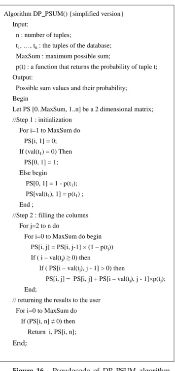
Algorithm DP_PSUM() {simplified version} Input:
n : number of tuples;
t1, …, tn : the tuples of the database;
MaxSum : maximum possible sum;
p(t) : a function that returns the probability of tuple t; Output:
Possible sum values and their probability; Begin
Let PS [0..MaxSum, 1..n] be a 2 dimensional matrix; //Step 1 : initialization
For i=1 to MaxSum do PS[i, 1] = 0; If (val(t1) = 0) Then PS[0, 1] = 1; Else begin PS[0, 1] = 1 - p(t1); PS[val(t1), 1] = p(t1) ; End ;
//Step 2 : filling the columns For j=2 to n do
For i=0 to MaxSum do begin PS[i, j] = PS[i, j-1] × (1 – p(tj))
If ( i – val(tj) ≥ 0) then
If ( PS[i – val(tj), j - 1] > 0) then
PS[i, j] = PS[i, j] + PS[i – val(tj), j - 1]×p(tj);
End;
// returning the results to the user For i=0 to MaxSum do If (PS[i, n] ≠ 0) then Return i, PS[i, n];
End;
Figure 16. Pseudocode of DP_PSUM algorithm for tuple-level model
proach for computing SUM we assumed that all tuples have the same number of possible aggr values. However, there may be cases where the number of possible aggr values in tuples is not the same. We deal with those cases as follows. Let t be the tuple with maximum number of possible aggr values. We set m to be equal to the number of possible values in t. For each other tuple t', let m' be the number of possible aggr values. If m'<m, we add (m - m') new distinct values to the set of possible values of t', and we set the probability of new values to zero. Obvi-ously, the new added values have no impact on the re-sults of ALL_SUM queries because their probability is zero. Thus, by this method, we make the number of pos-sible aggr values in all tuples equal to m, without impact-ing the results of ALL_SUM queries.
Appendix C: Pseudocode of AL_SUM algorithms
Figure 15 and Figure 16 show the pseudocode of the Q_PSUM and DP_PSUM algorithms.