Decoupled Capacity with Powerloop
byElisa Fankhauser
Bachelor of Science, Supply Chain Management & Finance, Arizona State University, 2015 and
Ge Li
Bachelor of Art, Supply Chain Management, Michigan State University, 2015 SUBMITTED TO THE PROGRAM IN SUPPLY CHAIN MANAGEMENT IN PARTIAL FULFILLMENT OF THE REQUIREMENTS FOR THE DEGREE OF
MASTER OF APPLIED SCIENCE IN SUPPLY CHAIN MANAGEMENT AT THE
MASSACHUSETTS INSTITUTE OF TECHNOLOGY JUNE 2019
© 2019 Elisa Fankhauser and Ge Li. All rights reserved.
The authors hereby grant to MIT permission to reproduce and to distribute publicly paper and electronic copies of this capstone document in whole or in part in any medium now known or hereafter created. Signature of Author: ____________________________________________________________________
Department of Supply Chain Management May 10, 2019 Signature of Author: ____________________________________________________________________ Department of Supply Chain Management
May 10, 2019 Certified by: __________________________________________________________________________ Lars Meyer Sanches Visiting Scholar Capstone Advisor Accepted by: __________________________________________________________________________
Dr. Yossi Sheffi Director, Center for Transportation and Logistics Elisha Gray II Professor of Engineering Systems Professor, Civil and Environmental Engineering
Decoupled Capacity with Powerloop by
Elisa Fankhauser and Ge Li
Submitted to the Program in Supply Chain Management on May 10, 2019 in Partial Fulfillment of the
Requirements for the Degree of Master of Applied Science in Supply Chain Management
ABSTRACT
With the current imbalance of supply and demand of truck drivers in the U.S., improving driver utilization is critical to secure reliable freight transportation. The largest source of downtime for carriers is the time spent at shippers’ facilities during the unloading and loading process, during which carriers might be detained for longer than two hours and fees charged to shippers. Powerloop provides an alternative model by allowing small carriers to participate in its trailer pool model that provides round trips to carriers and allows shippers to pre-load freight at their convenience. This improves the utilization of carriers by using dropped freight compared to the traditional live-load model. This project focuses on the benefit Powerloop provides to shippers, and assesses the quantitative impact of Powerloop on on-time delivery performance and detention fees. To model the expected on-time delivery and detention fees of Powerloop, we conducted a discrete event simulation by separating each activity during the load delivery process for both the traditional and Powerloop models. The simulation model results indicate that Powerloop loads have a 2% higher on-time delivery rate compared to the traditional live-load freight model, and can expect to save $11-16 per load in detention fees. As Powerloop moves along the learning curve and gains greater density through more customers, we expect these values to improve and provide and even greater benefit to shippers.
ACKNOWLEDGMENTS
We would like to thank our advisor, Lars Sanches, for providing guidance and support throughout this project. Also, we would like to thank our sponsoring company, Uber Freight, for generously connecting us to all the subject matter experts for interviews and committing time every week to provide feedback, suggestions, and guidance. Next, we want to thank Terianne Hall for helping us test different distributions with the Python fitter package. We would also like to thank Toby Gooley and Pamela Siska for reviewing our reports numerous times and providing detailed feedback over areas of improvement. Lastly, we both would like to thank our family, colleagues, and CTL faculty members for always being supportive to our spirit and this project.
TABLE OF CONTENTS
List of Figures ... 6
List of Tables ... 7
1. INTRODUCTION ... 8
1.1 Background and Motivation ... 8
1.2 Problem Statement ... 12
1.3 Methodology ... 12
1.4 Conclusion ... 13
2. LITERATURE REVIEW ... 14
2.1 Universal Trailer Pools ... 14
2.2 Powerloop ... 16 2.3 Exploration of Detention ... 18 2.4 Methodology Selection ... 18 3. METHODOLOGY ... 20 3.1 Expert Interviews ... 20 3.2 Data ... 22 3.2.1 Data Types ... 22 3.2.1 Data Integrity ... 23
3.2.1 Data Cleaning and Assumptions ... 23
3.3 Discrete-Event Simulation Model ... 24
3.3.1 Detention Time Simulations... 25
3.3.1.1 Triangular and Normal Distributions ... 26
3.3.1.2 Additional Distributions ... 28
3.3.1.3 Heuristic Method ... 32
3.3.2 Transit ... 34
3.3.3 Hours of Service ... 34
3.3.4 Performance Metric Assumptions and Calculations ... 35
3.3.5 Model Compilations ... 37
3.3.6 Model Limitations ... 38
4. RESULTS AND ANALYSIS ... 41
4.1 On-Time Delivery (OTD) Rate Performance ... 41
4.2 Detention Fee Savings ... 42
4.3 Additional Finding ... 44
5. RECOMMENDATIONS ... 46
6. CONCLUSION ... 47
REFERENCES ... 49
LIST OF FIGURES
Figure 1. Texas Triangle ... 11
Figure 2. Traditional loads... 16
Figure 3. Powerloop loads ... 16
Figure 4. Powerloop Operations Options ... 20
Figure 5. Timestamps in the Dataset ... 21
Figure 6. Discrete events in load execution ... 24
Figure 7. Simulated Triangular Distribution Time vs. Real Distribution Time ... 26
Figure 8. Simulated Normal Distribution Time vs. Real Distribution Time ... 27
Figure 9. Distribution fitter outputs against actual detention including outliers ... 28
Figure 10. Distribution fitter outputs against actual detention excluding outliers of greater than 10 hours for all scenarios and less than 30 minutes for live scenarios ... 29
Figure 11. Live-live pickup Log-Laplace and Real Distribution Comparison ... 31
Figure 12. Simulated PDFs in Each Scenario at Pickup Facilities ... 32
Figure 13. Simulated PDFs in Each Scenario at Drop-off Facilities ... 32
Figure 14. Hours of Service Demonstration ... 34
Figure 15. Simulation Model Logic ... 36
Figure 16. OTD Performance Comparison ... 40
Figure 17. Simulated Detention Fee per Shipper per Year Waterfall Comparison ... 41
Figure 18. Simulated Detention Fees Per Load Comparison ... 42
LIST OF TABLES
Table 1: Glossary of Terms ... 11 Table 2: Simulatiom Model Flow ... 316
1. INTRODUCTION
In this section, we introduce the background of Powerloop, which is our subject of study and a potential solution to the driver shortage that is creating a bottleneck for the trucking industry. With help from our sponsor company, which has expertise and technology for optimizing transportation routes, our study focused on quantifying the benefits of deploying Powerloop for the shippers. We also gave a high-level introduction of the problem statement, methodology, and conclusion in this section with details included in the following sections of the report.
1.1 Background and Motivation
The North American truckload market is worth over $700B (American Trucking Associations, 2018), and while load booking historically has been done more with long-term contracts, the market is now shifting to an increasing number of loads being booked on the spot market, which increases the uncertainties and costs to shippers. Additionally, the increasing shortage of truck drivers combined with inefficiencies of driver utilization, which we define as the portion of time a driver spends in transit versus waiting at a shipper facility, have become major bottlenecks in the trucking industry (Costello & Suarez, 2015).
The current freight landscape has an imbalance of supply and demand, with a shortage of drivers being one of the most significant challenges faced by the freight industry. According to the American Trucking Associations (2017), there was a shortage of approximately 50,000 truck drivers in the U.S. in 2017, and some large carriers are refusing as much as 1800 loads a day due to lack of available drivers (Koke, 2015). The majority of carriers in the truckload market are small carriers, often single-operator owned (American Trucking Associations, n.d.). The limited supply of carriers has contributed to an increase in freight costs
and made it more difficult to match carriers and shippers, decreasing the marketplace liquidity, which we define as the ease of booking freight at a transparent price (Helguera & Mukti, 2018).
Additionally, driver utilization has been affected by the implementation of the Electronic Logging Device (ELD) statute in December 2017, which logs the Hours of Service (HOS) of a driver (Sterk, 2018). This ensures drivers will be in compliance with the limit of the number of hours they can spend on the road, and led to a 5-15% increase in spot rates after the implementation (Sterk, 2018).
Another issue affecting carrier utilization is the amount of time carriers spend at shipper facilities, or detention time. Typically, carriers spend around two hours at shipper and receiver facilities for loading and unloading, which represents loss of value-add time that carriers could spend transporting freight. It is not uncommon, however, for carriers to spend much longer than two hours at a facility. This time spent at facilities not only affects the number of loads a carrier can take, but also impacts the shipper by increasing the potential for the load to arrive late at the receiver and increasing financial costs associated with detention fees. Typically, shippers are charged between $25-$90 hour for detention after the first two hours (Sullivan, 2015). Given the driver shortage, ELD mandate, and the number of hours carriers spend at shipper facilities, there is a need to maximize driver and asset utilization and minimize overall transportation costs.
Powerloop presents a solution to these issues and creates beneficial outcomes for both carriers and shippers. Powerloop is an affiliate of the sponsor company, Uber Freight, and is a home-grown universal trailer program that allows small carriers to participate by using their own power units and renting Powerloop trailers. Powerloop also provides round trips for carriers, improving the attractiveness of the loads as drivers can return home at the end of the day as opposed to on the road. Carriers pick up
pre-loaded trailers from shippers, reducing the time spent at the shipper facility to just the time needed to hook up to the pre-loaded trailer. This improves carrier utilization and has the potential to relieve pressure on the imbalance of supply and demand. Powerloop also potentially decreases for delays and detention fees (Table 1) while improving the outlook for on-time delivery. Both shippers and carriers benefit, as carriers are able to take more loads and improve their profit, while shippers can see improvements in on-time delivery (OTD) performance and cost (Table 1). Figures 2 & 3 in the Literature Review provide graphic representations of the differences in process between Powerloop and traditional loads.
While this project aims to quantify the benefit shippers can realize by participating in Powerloop in regards to on-time delivery performance and detention fees, there are other benefits to shippers. By allowing shippers to pre-load trailers at their convenience, shippers can better utilize their labor force, as they are not constrained by the two-hour loading windows of typical freight. This allows for improvements in warehousing efficiency and labor utilization, in addition to the detention fee savings and improved on-time delivery (Table 1).
Table 1. Glossary of Terms
Name Description
Power unit,
tractor Head of the truck that contains the engine and driver’s cab that is used to pull the trailer. Trailer Container on wheels that contains the freight.
Live
load/unload Carrier brings trailer to the shipper facility and waits for it to be loaded/unloaded. Carrier departs with both the power unit and trailer of loaded/unloaded freight. Dropped load
(at pickup) Trailer is pre-loaded prior to the carrier’s arrival. These trailers are dropped at the shipper facility prior to the carrier’s pickup time.
Dropped load
(at receiver) Trailer is dropped off at the receiver facility and unloaded at the convenience of the shipper. Carrier leaves with just the power unit after making the delivery.
Schedule type – Appointment
Appointment: indicates there is a specific time the carrier is scheduled to arrive. Typically, shippers will allow a 30-minute grace period after the appointment time before the carrier is considered late.
Schedule type – Window
Window: a larger time frame is allowed for the carrier to arrive, sometimes spanning up to 24 hours. The carrier can arrive at any time during the window and be considered on-time.
On-Time
Delivery (OTD) Metric indicating whether or not the freight was delivered to the receiver by the specified appointment time or window.
Accessorial fees Fees incurred by shippers and paid to carriers for performing freight services beyond the normal pickup and delivery, including excess waiting time (detention fees), redelivery, layovers, lumper (third parties hired by shippers to load or unload trailers), fuel surcharges, or truck ordered not used (TONU).
Detention The time a carrier spends at a shipper or receiver facility waiting for freight to be released, typically while freight is being loaded or unloaded.
Detention fees
Fees incurred by the shipper and paid to the carrier for exceeding the agreed upon time limit for keeping the trailer at a shipper or receiver facility. Typically, two hours of time is allotted at the shipper and receiver end during a live-load scenario. Any additional time the carrier spends at the facility incurs fees, usually around $50-$75 an hour.
1.2 Problem statement
This project aims to simulate the expected on-time delivery and detention fees shippers can expect by participating in Powerloop. While Powerloop plans to expand to multiple regions, the project will focus on the “Texas Triangle”, or loads between Dallas, Houston, and San Antonio (Figure 1).
Figure 1. Texas Triangle 1.3 Methodology
To conduct the research, we had approximately twenty 30-minute interviews with the industry or operational experts within the sponsoring company to understand the trucking industry background and the value-adding of this study. Upon the completion of refining the scope, we requested operational data and cleaned it to build a better foundation of the later model building. Meanwhile, we explored literature and decided to utilize discrete-event simulation as our main approach to simulate the processes of both traditional Uber Freight and Powerloop loads in order to compare each event between the two models. In the end, we concluded our findings based on the model and delivered the model to the sponsoring company for future delivery scheduling. This model allows the sponsoring company to schedule the delivery windows with more accuracy based on the scientific calculations.
1.4 Conclusion
From the simulated result, we conclude that Powerloop would improve the delivery performance over the on-time rates by 2% at this early stage of operation and reduce detention fees charged on both shippers’ and carriers’ sides by an average of $16 per load. Of the three scenarios in the current operations, drop-drop scenario performs the best, followed by drop-live and then live-live. This confirms our expectation that when we reduce the detention time at the facilities by saving the time for live loading and unloading, the truck idle time would be reduced and lead to better on-time rates. Also, the penalty fees of detention would be reduced as well with less detention time.
2. LITERATURE REVIEW
In this Capstone, we focus on quantifying expected detention fees and on-time delivery (OTD) performance for shippers participating in Powerloop. To understand how Powerloop could affect shippers in regard to these attributes, we started by reviewing existing literature to explore the history of the drop and hook, which is the practice of decoupling trailers and tractors, typically through a universal trailer pool. This allows trailers to be dropped at shipper facilities and pre-loaded or unloaded at the convenience of the shipper rather than within the two-hour time frame typically allowed for live-load models. Then we looked at Powerloop’s model to identify how it differs from the traditional universal trailer-pool model. Lastly, in order to compare and contrast the two operational models, we researched existing methodologies to simulate the activities and identified discrete-event simulation as the most appropriate methodology for this project.
2.1 Universal trailer pools
Although Powerloop is a new program in the freight industry, its roots come from a universal trailer pool model that exists in the freight industry. Some large carriers utilize universal trailer pools by having a large pool of trailers that they allocate across shippers in a given geography. These trailers can be pre-loaded by shippers, and then picked up by drivers who arrive with just the power unit, which is the tractor that attaches to the trailer to move the load. The trailers might be dropped off at the receiver facility with the driver leaving with just their power unit, or they might be live unloaded with the driving taking both the power unit and trailer to the next destination. Large shippers, such as Coca-Cola, also employ internal trailer pools to capture advantages from using dropped trailers (Albright, 2013). These companies have their own fleet of trailers that flow between their shipper and receiver facilities, and either employ their own drivers or contract out loads to for-hire carriers.
There are many benefits to using dropped trailers through trailer pools. First, shippers can pre-load trailers at their convenience and are not constricted to the two-hour window typically allowed through a live-load process (Ackerman, 2013). This allows shippers to better utilize labor, as they can load the trailer during slow times at the warehouse. It can also free up space on the dock, as pallets can be loaded onto a trailer as soon as they are ready instead of being staged on the dock until the trailer arrives to be live loaded (IFCO Systems, 2017). Second, shippers can reduce detention fees paid to carriers (Ackerman, 2013). It is common for live loading to take longer than two hours, after which detention fees are charged. Typical detention fees can cost shippers between $25- $90 an hour after the first two hours and up to $300 for layover fees if the driver needs to remain at the facility overnight (Sullivan, 2015). By pre-loading trailers, shippers can mitigate these fees, as the carrier only needs to attach their power unit to the trailer before taking off for the destination. A study on a retail distributor found that the time carriers spent at a facility was reduced by 46% after the distributor switched to using dropped trailers (Speredelozzi, Hassanzadeh, Wolf, & Holwitt, 2006). Lastly, it can also make the shipper more attractive to carriers, as carriers can have better assurance that they will not spend unnecessary time at facilities waiting for loads to be ready and can in turn make more profit from taking additional loads (Uber Freight, personal communication).
This attractiveness to carriers is becoming increasingly important, as the shortage of drivers in the trucking industry means that shippers that are preferred by carriers are more likely to get loads booked more easily and efficiently (Schneider, 2018). According to interviews with the sponsoring company, many carriers give priority to shippers who provide better experiences. These better experiences could come in the form of shippers providing waiting areas with amenities, shorter wait times, better treatment by the facility staff, or more favorable lanes (Uber Freight, personal communication).
2.2 Powerloop
Powerloop differs from traditional universal trailer pool models in a few ways. First, unlike organizations that utilize internal trailer pools, Powerloop is offered commercially. This helps reduce the asset investment requirement from shippers who might otherwise need to procure their own trailers for an internal program (Bensinger, 2018).
Second, Powerloop allows any carrier contracted with them to participate in the program. Typically, only large carriers are able to participate in such a program, as a certain level of load density and volume is required to make it profitable (Pike & Asante, 2018). A small carrier is typically unable to make the capital investment needed to have excess trailers stored at shipper facilities for pre-loading. By allowing carriers to use Powerloop trailers, the barrier to entry for carriers is vastly reduced and creates greater marketplace liquidity for the program, as Powerloop has access to a large carrier pool compared to programs that only allow direct employees to operate trailers.
Thirdly, Powerloop provides round trips to carriers compared to the typical one-leg load. Instead of merely offering a load from point A to point B, Powerloop will schedule a series of loads that allows the driver to end back in the region of point A. This increases the attractiveness of Powerloop to carriers, as many drivers would like to spend their evenings in their own home as opposed to on the road. In instances where this is not possible or when the driver does not wish to come back to point A, carriers can rent Powerloop trailers for $25 a day to find and deliver their own loads with an agreement to deliver the trailer back to a specified location after an agreed upon amount of time (Uber Freight, 2018).
Given the current imbalance of supply and demand from a lack of drivers, shippers and carrier programs need to be able to attract drivers to gain competitive advantage. By spending less time at shipper facilities
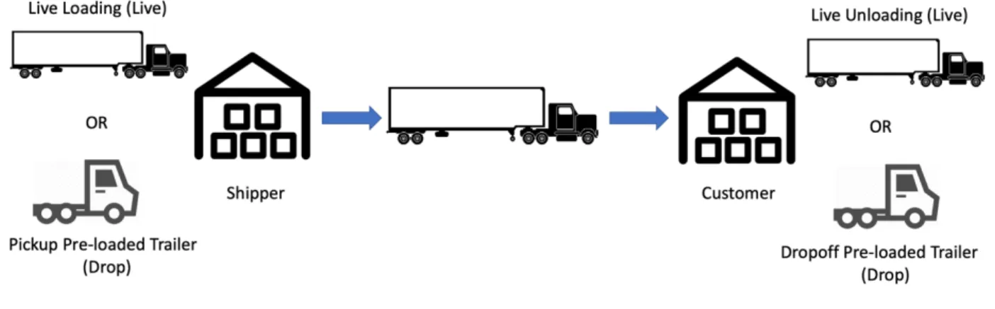
waiting to be loaded, carriers spend more time on the road and can complete their trips in a shorter time frame, allowing them to take more loads, increase their profits, and accept loads at lower rates. Powerloop’s attractiveness to carriers ensures they will have a healthy supply of drivers and gives them a competitive advantage over other programs. Figures 2 and 3 demonstrate the traditional live-load model compared to Powerloop’s model.
Figure 2. Traditional loads ~ 2 hrs. live-load
Shipper A Receiver B
~2 hrs. live-unload Travel time
Traditional loads are completed with carriers providing both the power unit and the trailer. Carrier arrives at shipper facility at point A and the trailer is loaded, typically taking around two hours. Carrier then drives to point B and is unloaded, taking approximately two hours. The carrier needs to find its own backhaul load, which will follow the same model.
Source: Uber Freight, Personal Communication, August 2018
Shipper A Receiver B
Shipper C Receiver D
~15 min to attach to
pre-loaded trailer Option 1: ~15 min to drop trailerOption 2: ~ 2 hr. to live unload
Option 1: ~15 min to drop trailer
Option 2: ~ 2 hr. to live unload ~15 min to attach to pre-loaded trailerto attach to pre-loaded trailer min Arrive with just the
power unit Travel time
Travel time
In the Powerloop model, the carrier arrives at the shipper facility at point A with just the power unit. The carriers picks up a dropped trailer and departs the building, which takes around fifteen minutes. The carrier drives to the receiver facility in point B, where it might either drop the trailer or be live-unloaded. The carrier is provided a similar back haul load from somewhere in point B back to point A.
2.3 Exploration of Detention
As discussed in the above sections, detention time and the associated fees represent a key challenge in the freight industry. In a freight survey from DAT Solutions (2016), a provider of U.S. transportation information, 63% of drivers reported that they typically spend more than three hours at facilities for the loading or unloading process. Fees charged to shippers can be anywhere from $25-$90 per hour after the first two hours, so this additional detention time at facilities can be costly to both shippers and carriers (Sullivan, 2015). Shippers end up paying additional fees for their loads, and carriers might miss their next load and forfeit income. This further contributes to the driver underutilization problem as well, as detained drivers spend less time on the road transporting freight and more time waiting at facilities. Shippers recognize this is an issue, as 20% of the shippers in the survey reported detention among their top five issues, while the majority of shippers noted that it was an issue but other challenges took priority (DAT Solutions, 2016). This provides an opportunity for Powerloop to assist shippers, as it is a passive way for shippers to reduce their detention without significant effort on their end. For carriers, detention signaled an even larger problem, with 84% of carriers reporting detention as one of the top five business problems (DAT Solutions, 2016). As the supply of drivers continues to shrink, a key issue will be how to increase the utilization of existing carriers and entice carriers to deliver to shipper facilities.
2.4 Methodology Selection
Although there is existing research on dropped trailers and trailer pools, there is limited research on its impact on on-time delivery and detention fees, particularly for the specific process that Powerloop employs. To identify potential methodologies that could simulate the impact in these areas, we looked at academic articles on simulation model comparisons. We found that discrete-event simulation (DES) would be an appropriate method to implement. Discrete-event simulation models the operations of a system in
a series of discrete events that encompasses the various processes in the system, with no changes expected in the system between sequential steps (Robinson, 2004).
Jahangirian, Eldabi, Naseer, Stergioulas, and Young (2010) summarized 281 academic articles and journals to show that DES was the most popular model in simulating manufacturing and transportation processes, with 40% of the papers reviewed using it to study and analyze detailed processes. System Dynamics (SD) was the second most popular model, selected by over 15% of the sample. According to the study, DES is preferred by many scholars for the convenience it brings (Jahangirian et al., 2010).
To validate our initial hypothesis that DES would be more favorable for this project than SD, we also looked at when each model should be applied. Both models are broadly used among researchers for manufacturing settings, but their different attributes make them suitable for different research purposes. For example, DES uses statistical distributions to generate randomness, while SD uses average values to reflect the flows. Therefore, DES is more suitable for operational- or tactical-level studies while SD is for strategic levels (Tako & Robinson, 2012). Because the aim of this project is to understand the detention fee savings and OTD improvement of shippers participating in Powerloop, we need to look at the operational level processes, indicating DES is a more appropriate methodology for this project.
Another benefit of DES is that by simulating each event in the overall process, costs incurred in each step can be more easily calculated and attributed to a specific cost driver. The information generated from this can be incorporated into activity-based costing (ABC) analyses, which allocates operational cost into individual activities to understand the cost efficiency of each activity and is commonly used in the supply chain management (Spedding & Sun, 1999). For these reasons, DES is the best model to implement for
the purpose of quantifying detention fee savings and on-time delivery performance for shippers participating in Powerloop.
3. METHODOLOGY
To study the impact of Powerloop on detention fees and on-time delivery performance, we first began by conducting qualitative research with the sponsor company, Uber Freight. We conducted interviews with team members to better understand the freight industry and background of Powerloop. We then examined and cleaned the available data from the sponsor company, specifically data regarding the time carriers spend at shipper facilities and in transit for Powerloop loads (round-trip dropped loads) and regular Uber Freight loads (one-way live-loads). Next, we conducted a statistical analysis on the distributions of the time spent for each operational activity during the load deliveries. Lastly, we built the simulation model based on the distributions for each activity to estimate the expected on-time performance and detention fees. The following sections will dive more into the details of our methodology.
3.1 Expert Interviews
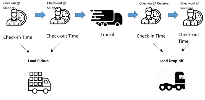
To gain a better understanding of Powerloop, we conducted twenty 30-minute interviews with Powerloop and Uber Freight team members and customers. During interviews with the Powerloop program manager, we gathered information on the different types of loads. Currently, there are four different combinations of Powerloop loads, although only two are common. Figure 4 illustrates these different loads. The two most common Powerloop loads are drop-live (pre-loaded, dropped trailer is picked up at receiver, live-unloaded at receiver), and drop-drop (pre-loaded, dropped trailer is picked up at receiver, trailer is dropped at receiver). While uncommon, there are instances of live-drop (trailer is live-loaded at shipper,
Figure 4. Powerloop Operations Options
The most preferable load by Powerloop currently is drop-live, as trailers need to be freed up in a timely manner after drop-off to ensure there are enough available trailers in the pool. If a receiver holds on to a dropped trailer for an extended amount of time, it affects the rest of the trailer pool negatively by decreasing the amount of available assets. In this case, drop-live helps improve the overall flow of the trailers.
For pickup at the shipper facility and drop-off at the receiver facility, the predetermined arrival schedule can be either an appointment time or a window. For appointments, a specific time is set that determines when the carrier needs to arrive. There is usually a grace time of 30 minutes, after which the carrier is considered late. If the carrier arrives on time, detention fees would begin to incur two hours after the appointment time starts, regardless of whether or not the carrier arrived early. For example, if a shipper has an appointment time of 10:00 a.m. and the carrier arrived at 9:30 a.m., detention would not start until 12:00 p.m. The other type of schedule is a window, which is a wider time frame in which the carrier can arrive at any point of time during the window to be considered on-time. Some windows are as large as 24 hours. Assuming the carrier is on-time, detention would start two hours after the carrier arrival time.
3.2 Data
We were provided six months of data for both Uber Freight and Powerloop loads, which contained the essential data points for mapping out the processes and comparing between the two operating modes using a discrete-event simulation model. Since Powerloop was launched in Fall 2018, there was only approximately six months of data regarding Powerloop loads. To make the data comparable, we requested Uber Freight’s data during the same time frame. In the following sections we will introduce the data elements provided, data challenges, and the cleaning process and assumptions.
3.2.1 Data Types
The primary data included are as following.
• Trip Identifiers – Unique ID numbers of the loads, carriers, and shippers. This information could help with creating scenarios based on the delivery information of each unique shipper or carrier to further explore differences between different operating modes.
• Trip Types – Designates appointment or window, traditional freight or Powerloop, and live-live, drop-live, or drop-drop scenarios.
• Timestamps – Includes timestamps of carrier check-in and check-out times at the shipper and receiver facilities for both operating modes of traditional freight and Powerloop (Figure 5). It includes both the actual check-in and out times as well as the scheduled appointment and window times, which is used for calculating detention fees and on-time pickup and delivery rates.
• Geographic Information – Travel distances of each trip and the latitude and longitude of shipper facilities, and source and destination cities and regions.
• On-Time Rates and Detention Fees – Actual on-time pickup and drop-off delivery rates and detention fees paid to the carriers for each load.
3.2.2 Data Integrity
The data provided by Uber Freight represents actual loads for both Uber Freight and Powerloop. This data contains the time spent at each activity during a load, including the time spent at a shipper facility for loading and unloading, and time in transit. Some of the values require driver input, such as the check-in arrival time at a shipper facility. As a result, there is a possibility of human error affecting the dataset. The time spent at facilities is also affected by the number of docks at a particular shipper and the efficiency of the dock and yard management, which is not reflected in the dataset as individual features. Additionally, Powerloop loads have more limitations placed on them compared to Uber Freight loads, such as geographic region and manual booking. To reduce the impact of these factors, we made a variety of assumptions for both data cleaning and model building, which will be discussed in the next sections.
3.2.3 Data Cleaning and Assumptions
To achieve greater data integrity and fair comparisons between the two operating models, we made the following assumptions during the data cleaning process:
1. Limited data from the same region for both models. Powerloop is only operating in the Texas triangle area of Fort Worth, Dallas, Houston, Austin, and San Antonio. To compare the two models more fairly, we limited the data to this region for both models.
2. Removed rows with null timestamp values. The model is dependent on the timestamp values to simulate the two freight models, and therefore data lacking timestamps is not reliable.
3. Limited data to loads coordinated through the operations team and excluded app-based loads. Powerloop does not utilize the mobile app to schedule loads yet and relies only on the operations team to coordinate them, and to compare the two models more fairly we limited the normal freight data to loads booked through the operations team.
4. Removed trailer repositioning loads. Trailer repositioning loads represent loads in which trailers are moved from one facility to another to ensure the proper number of trailers are positioned at the correct shipper facilities for Powerloop. These loads do not contain freight, and are not representative of the delivery ecosystem.
3.3 Discrete-Event Simulation Model
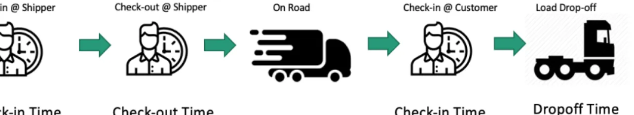
Discrete-event simulation models the operations of a system in a series of discrete events that encompasses the various processes in the system, with no changes expected in the system between sequential steps. The process of Uber Freight and Powerloop loads can be broken out into discrete events shown in Figure 6, representing the carrier check-in and check-out times at the shipper facility, transit time, and the carrier check-in and check-out times at the receiver facility. After modeling these events, the expected on-time delivery, total detention time, and total detention fees incurred in the system can be calculated.
Figure 6. Discrete events in load execution
The key difference between the traditional Uber Freight and Powerloop loads is the time spent between check-in and check-out at the shipper and receiver facilities. Under the live/live scenario, the time spent at facilities is longer compared to drop/drop and drop/live, as the freight needs to be loaded and unloaded at both the pick-up and drop-off facilities.
3.3.1 Detention Time Distribution
To simulate the detention time, or the time a carrier spends at a shipper facility for the loading or unloading process, we first tried to fit each time distribution into a common distribution that best represent the characteristics. We started from the most commonly applied distributions (triangular and normal), followed by 80 types of distributions with Python fitter package, then used the probability density function (PDF) as a heuristic method to simulate random detention times as none of the statistical distributions produced a statistically good fit for the actual time distributions. The following subsections go into detail about the studies we conducted on the distribution.
Check-in @
Shipper Check-out @ Shipper Check-in @ Receiver Check-out @ Receiver
Check-in Time Check-out Time Transit Check-in Time Check-out Time
3.3.1.1 Triangular and Normal Distributions
We started by trying fitting triangular and normal distributions to the detention time distributions since these two statistical distributions require the least amount of data and are commonly used in practical business.
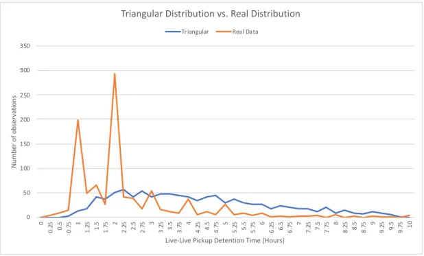
Triangular distribution is commonly used to model asymmetric distributions that have a long right tail with no negative values. Hence, for live-live scenario, we used a minimum time of 0.5 hours, mode of 2 hours, and a maximum of 10 hours as parameters to generate random numbers for the simulation.
DetentionTime = a + -. ∗ (1 − 3) ∗ (5 − 3) 67 . ≤ 5 − 3 1 − 3 9:;:<;6=<>6?: = c − -(1 − .) ∗ (1 − 3 ) ∗ (1 − 5) 67 . ≥ 5 − 31 − 3
Where
r = random number generated between (0,1) a = minimum detention time
b = mode detention time c = maximum detention time
However, the drawback of the triangular distribution and the key reason we did not utilize it is that it tries to fit the right tail values into the triangle of the three parameters. Since the actual time distribution has a right tail close to zero, triangular distribution would overestimate the right tail values and result in higher representation of extremely long detention times (Figure 7). It also underestimates the frequency of the mode detention time. In this case, we decided that triangular distribution does not fit well for the simulation model.
Figure 7. Simulated Triangular Distribution Time vs. Real Distribution Time
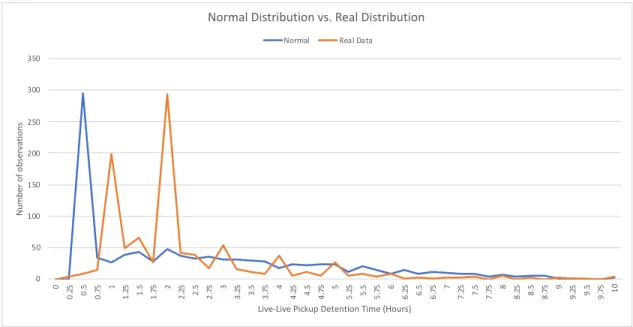
Then we tried normal distribution by limiting the minimum to 0.5 hours with a mean of 2 hours and standard deviation of 2.8 hours. The resulting random numbers do not represent the actual distribution well either, as the distribution tends to create a peak at 0.5 hours because we manually set all potential values below the minimum possible time at the minimum (Figure 8). Then the normal distribution would underrepresent the two peaks at 1 and 2 hours and smooth out the entire distribution. Therefore, the normal distribution would not be appropriate as well.
0 50 100 150 200 250 300 350 0 0. 25 0.5 0. 75 1 1. 25 1.5 1. 75 2 2. 25 2.5 2. 75 3 3. 25 3.5 3. 75 4 4. 25 4.5 4. 75 5 5. 25 5.5 5. 75 6 6. 25 6.5 6. 75 7 7. 25 7.5 7. 75 8 8. 25 8.5 8. 75 9 9. 25 9.5 9. 75 10 N umb er o f o bse rv ati on s
Live-Live Pickup Detention Time (Hours) Triangular Distribution vs. Real Distribution
Figure 8. Simulated Normal Distribution Time vs. Real Distribution Time
3.3.1.2 Additional Distributions
We next explored various distribution types that fit the detention time for each scenario. We first mapped the current distribution of detention times for live/live, drop/drop, and drop/live loads (Figures 8 and 9). To gain an understanding of how outliers affect the distribution, we graphed the data including outliers, and charted it against the five best distribution fits out of 80 distribution types (Figure 8). Appendix B contains a list of all the distributions tested.
0 50 100 150 200 250 300 350 0 0. 25 0.5 0. 75 1 1. 25 1.5 1. 75 2 2. 25 2.5 2. 75 3 3. 25 3.5 3. 75 4 4. 25 4.5 4. 75 5 5. 25 5.5 5. 75 6 6. 25 6.5 6. 75 7 7. 25 7.5 7. 75 8 8. 25 8.5 8. 75 9 9. 25 9.5 9. 75 10 N umb er o f o bse rv ati on s
Live-Live Pickup Detention Time (Hours)
Normal Distribution vs. Real Distribution
Figure 9. Distribution fitter outputs against actual detention including outliers
We next graphed the distributions excluding outliers (Figure 10). After conducting interviews with operations on outliers, detention times greater than 10 hours for all scenarios were removed, and detention time less than 30 minutes for live-load scenarios were removed. In all scenarios, detention time greater than 10 hours is very rare and typically represents human entry error. For traditional live-live
loads, less than 30 minutes is generally not feasible as the trailer needs to be backed into a dock, examined to ensure it is safe to enter, and manually loaded.
Figure 10. Distribution fitter outputs against actual detention excluding outliers of greater than 10 hours for all scenarios and less than 30 minutes for live scenarios
The actual distribution of detention times for all scenarios generally peaks at 30-minute and 60-minute intervals. Check-in and check-out times are manually entered by drivers, who tend to enter even values corresponding to common time intervals.
To test how well the distributions fit the data sets, we conducted chi-square tests, which tests how well a statistical distribution fits a data set. The test evaluates a null hypothesis that the data is explained by a distribution against the alternative that it is not, and is typically in the following form.
CD= E(F5G:.H:I − :JK:1;:I)D
:JK:1;:I
We generated random numbers using the top five distributions for each load scenario and tested it against the actual values. After analyzing the results of the chi-squared tests, none of the distributions had a critical value that indicated the distribution accurately fit the data with p-values less than 0.00001, which allow us to reject the null hypothesis that the distributions has no significant differences between the observed (tested) and expected (actual) values. Figure 11 shows log-Laplace, one of the top five distributions for live/live pickup, against the actual distribution of data. The log-Laplace distribution overestimates the values that fall before 1 hour and underestimates the values around the 2-hour point.
Figure 11. Live-live pickup Log-Laplace and Real Distribution Comparison
Key factors that contributed to no adequate distribution types are the peaks that occur in the data around 30-minute increments, the absence of negative values as time is always positive, and the long right tails. Because no distribution type adequately explained the data, we decided to use a heuristic to simulate the distribution of detention time by using a probability density function (PDF) of the actual detention times.
3.3.1.3 Heuristic Method
The probability density function (PDF) represents the probability of having detention time fall under specific time frames, which we binned into 15-minute intervals. The selection of the time interval (bin) width considered that a smaller bin increases the possibility of overfitting the data while a larger bin would potentially bias the final result of the on-time rates and detention fees. Hence, we decided that 15-minute intervals would be the best fit for our study purposes.
0 100 200 300 400 500 600 700 0 0. 25 0.5 0. 75 1 1. 25 1.5 1. 75 2 2. 25 2.5 2. 75 3 3. 25 3.5 3. 75 4 4. 25 4.5 4. 75 5 5. 25 5.5 5. 75 6 6. 25 6.5 6. 75 7 7. 25 7.5 7. 75 8 8. 25 8.5 8. 75 9 9. 25 9.5 9. 75 10 N umb er o f o bse rv ati on s
Live-Live Pickup Detention Time (Hours)
LogLaplace Distribution vs. Real Distribution
Next, we calculated the PDFs in each 15-minute interval ranging from 0-10 hours of each scenario and used the random number generation add-in tool of Excel to simulate random detention times of 10,000 loads (both pickup and drop-off) to represent the possible detention outcomes. The resulting distribution very closely represented the actual detention times with most of the PDFs perfectly matching the actuals and a few of them only less than 1% off the actual. Figure 12 and 13 shows the PDFs of each simulated scenario.
Figure 12. Simulated PDFs in Each Scenario at Pickup Facilities
Figure 13. Simulated PDFs in Each Scenario at Drop-off Facilities 0% 5% 10% 15% 20% 25% 30% 35% 0. 25 0.5 0.75 1 1. 25 1.5 1.75 2 2. 25 2.5 2.75 3 3. 25 3.5 3.75 4 4. 25 4.5 4.75 5 5. 25 5.5 5.75 6 6. 25 6.5 6.75 7 7. 25 7.5 7.75 8 8. 25 8.5 8.75 9 9. 25 9.5 9.75 10 Pickup PDF Comparison
Pickup Live-Live Pickup Drop-Drop Pickup Drop-Live
0% 5% 10% 15% 20% 25% 30% 35% 0. 25 0.5 0.75 1 1. 25 1.5 1.75 2 2. 25 2.5 2.75 3 3. 25 3.5 3.75 4 4. 25 4.5 4.75 5 5. 25 5.5 5.75 6 6. 25 6.5 6.75 7 7. 25 7.5 7.75 8 8. 25 8.5 8.75 9 9. 25 9.5 9.75 10 Dropoff PDF Comparison
This exercise helped the model to generate a very close on-time rate and detention fees to the actual scenarios. There is, however, a potential of overfitting since the random numbers were generated based on the actual performance to reflect the current differences. We decided that the tradeoff between the improving accuracy and reducing overfitting risks, the accuracy is more critical for this simulation model to project the real benefit of Powerloop. Furthermore, the model would allow new simulations to be run with updated PDFs going forward to keep the results up-to-date so it could catch the progress made along the learning curve.
3.3.2 Transit
The Federal Highway Administration (2010) measures average trucking speed to be between 50-60 mph on interstate highways in the Texas Triangle, but this does not include driving required on urban or rural non-interstate roads, or the delays a truck incurs when stopping to refuel or for inspections. Based on feedback from Uber Freight and a carrier who works with Uber Freight, we selected 47 mph as the transit speed assumption in the model to account for non-highway driving and transit pauses. For the purposes of the model, we assume the transit speed is constant and does not vary based on peak hours, specific route geography, or driver behavior.
>.3<G6; ;6?: = ?6L:G/47
3.3.3 Hours of Service
Hours of service (HOS) requirements from U.S. Department of Transportation (2017) specifies that drivers need to take breaks after driving or being on-duty for a certain number of hours, demonstrated in Figure 14. Drivers must take a 30-minute break after eight hours of consecutive driving, and cannot drive more than 11 hours total while on duty. After they have driven for 11 hours or have been on duty for 14 hours, drivers must take a 10-hour break before resuming work.
In the model, carriers are assumed to arrive at the shipper facility with clean hours and begin accruing on-duty hours upon check-in. After each discrete event, the HOS constraints are checked to determine if the carrier needs to take a break before resuming work.
Figure 14. Hours of Service Demonstration
3.3.4 Performance Metric Assumptions and Calculations
The two principle metrics explored in this study are on-time delivery (OTD) performance and detention fees.
On-time performance is a binary calculation that measures whether or not a carrier arrived to the shipper by the scheduled arrival time. There are two different schedule types, appointment and window, and each have specifications for on-time performance:
OTDPQQRSTUVWTU = X0, =;ℎ:.b6G: 1, 67Zℎ:1\6< ≤ (]KK;^;3.; + 30?6<a;:G)
b.) Window: carrier is considered on-time only if it arrives within the window. No grace periods are allowed as the windows are typically generous, often spanning up to 24 hours.
OTDcSTdRc = X0, =;ℎ:.b6G: 1, 67Zℎ:1\6< ≤ (e6<I=bf<I)
Detention fees are incurred after a shipper detains a carrier for longer than the allotted free time, which is typically two hours. The following assumptions are built into the model:
a.) Detention fees are only incurred if the carrier arrives on time. If the carrier arrives late and detention time is greater than the grace period, the shipper will not be charged detention fees. b.) If the schedule type is an appointment, detention fees incur two hours after the start of the
appointment time, even if the carrier arrives early.
c.) If the schedule type is a window, detention fees incur two hours after the carrier arrives. d.) Detention fees are $60/hour with a $200 maximum fee.
3.3.5 Model Compilation
Figure 15 and Table 2 demonstrate the flow and logic of the simulation model; 10,000 loads of each scenario type (live-live, drop-drop, and drop-live) were simulated for the model.
Table 2. Simulation model flow Check-in at Shipper Derived from data provided by sponsor company
Check-out at Shipper !ℎ#$% − '( *+ ,ℎ'--#. + 0#+#(+'1( 2'3# *+ ,ℎ'--#.
Detention Time at Shipper Simulated from PDF distribution of detention time at the pickup facility described in section 3.3.1.3 Detention fees at shipper 0#+#(+'1(4## = 627
∗ 9(Detention ≥ 320 → 200) ∧ (120 < Detention < 320 → (Detention − 120) ∗ 1) ∧ 0J OTP
OTPKLLMNOPQROP = S0, 1+ℎ#.Z'Y# 1, 'U!ℎ#$%'( ≤ (W--+,+*.+ + 303'(X+#Y)
OTP[NO\M[ = S1, 'U!ℎ#$%'( ≤ (]'(^1Z_(^)0, 1+ℎ#.Z'Y#
HOS check See Figure 14.
Transit time 2.*(Y'+ +'3# = 3'`#Y/47
HOS check See Figure 14.
Check-in at Receiver !ℎ#$% − 1X+ *+ ,ℎ'--#. + 2.*(Y'+ 2'3#
Check-out at Receiver !ℎ#$% − '( *+ d#$#'e#. + 0#+#(+'1( 2'3# *+ d#$#'e#.
Detention Time at Receiver Derived from PDF distribution of detention at the drop-off location described in part 3.3.1.3 Detention Fees at Receiver 0#+#(+'1(4## = 620
∗ 9(Detention ≥ 320 → 200) ∧ (120 < Detention < 320 → (Detention − 120) ∗ 1) ∧ 0J
OTD OTD
KLLMNOPQROP = S0, 1+ℎ#.Z'Y# 1, 'U!ℎ#$%'( ≤ (W--+,+*.+ + 303'(X+#Y)
OTD[NO\M[ = S0, 1+ℎ#.Z'Y# 1, 'U!ℎ#$%'( ≤ (]'(^1Z_(^)
3.3.6 Model Limitations
There are various limitations to the model. First, the data set for Powerloop and Uber Freight were limited as Powerloop launched in Fall 2018. Given Powerloop is a new business, we expect that Powerloop performance will improve in the future as both operations and shippers move further down the learning curve. The distribution of detention times for Powerloop specifically will likely evolve in the future. Additionally, check-in and check-out times that are used to determine detention times and fees are manually recorded by carriers, increasing the chances for human error. There are peaks in the data at 30- and 60-minute increments, indicating that carriers are likely entering the nearest half hour as their check-in or check-out times. The actual distribution is likely smoothed between these two time check-intervals, complicating the accuracy of the dataset. The time spent at facilities is also affected by the number of docks at a particular shipper and the efficiency of the dock and yard management, which is a limitation of the model and an opportunity for further research.
Additionally, transit speed and carrier and shipper behavior are assumed as constant to provide simplicity in the mode. In actuality, carriers and shippers each exhibit different behaviors that affect detention. If a carrier drives slower than average and takes a long time to back into dock doors after check-in has occurred, this will increase detention. Transit speed is also highly dependent on traffic, geography of routes, and driver behavior. Although the ELD mandate has been in effect since December 2017, not all carriers in the Texas triangle have the devices installed, as older vehicles are not required to be equipped with the technology. There is a possibility that drivers might be going beyond the hours of service limits but reporting compliance with HOS by manually adjusting hours. This would bias the detention data for loads with these drivers, which is a limitation of the model.
The model also assumes shippers are charged for all incurred detention fees. In some instances, shippers might not be charged the fee in actuality or might decline to pay them, based on contractual agreements in either case. The real fees that shippers pay are likely below the calculated results.
Lastly, the simulation only looks at the Texas Triangle, as Powerloop is currently only operating in this region. Powerloop is expected to expand to other geographies, which will each have unique properties and characteristics that affect performance.
4. RESULTS & DISCUSSIONS
4.1 On-Time Delivery (OTD) Rate Improvement
After analysis of model simulation and actual data, we concluded that dropped freight results in higher on-time delivery rates compared to live-load freight. The overall on-time delivery (OTD) performance of the Powerloop drop-drop deliveries is 2% higher than that of the live-live loads in both the simulated environment and real data (Figure 16).
Figure 16. OTD Performance Comparison
Simulation observations:
• Scenarios that involve dropped freight have higher OTD rates than live-live scenarios. Live-load freight has higher overall detention times, resulting in a higher probability the carrier will not make it to the receiver facility on time. This is a compounding effect.
• Drop-drop scenarios have same OTD rates as drop-live scenarios. The load type at the receiver does not affect OTD performance because OTD is determined at the point of arrival and is agnostic to what occurs after the carrier has checked in.
Live-Live Drop-Drop Drop-Live
Appt Simulation 87% 90% 90% Window Simulation 92% 93% 93% Simulation Average 90% 92% 92% 84% 85% 86% 87% 88% 89% 90% 91% 92% 93% 94%
OTD Performance Comparison
• The simulated OTD is lower than the actual OTD. This is because the PDF was binned in 15-minute intervals and the random times generated selects the upper limit of the 15-minute intervals. This creates a slight bias of longer detention times, which led to lower OTD performance in the simulation model.
• Window schedule types have better OTD rates than appointment schedule types. Window schedule types allow carriers a greater range of time to arrive during which they are considered on time, making it easier for carriers to achieve higher OTD performance.
4.2 Detention Fee Savings
Similar to the on-time delivery analysis, drop-drop freight resulted in the most favorable detention fees in the simulation. The simulated drop-drop freight resulted in approximately $16 less in detention fees per load compared to live-live freight. For a shipper who executes 100 loads per day, the savings of utilizing the drop-drop freight would translate into $1,600 per day, or approximately $400K per year assuming 260 work days per year (Figure 17).
Figure 17. Simulated Detention Fee per Shipper per Year Waterfall Comparison
$892,320.00
$(307,320.00) $585,000.00
$(109,460.00) $475,540.00
Live-Live Savings of Drop-Live Drop-Live Savings of Drop-Drop Drop-Drop $-$100,000.00 $200,000.00 $300,000.00 $400,000.00 $500,000.00 $600,000.00 $700,000.00 $800,000.00 $900,000.00 $1,000,000.00
Figure 18 demonstrates the simulated and expected actual detention fees per load for each of the live-live, drop-drop, and drop-live scenarios. The expected actual fees represent what Uber Freight’s shippers actually incurred using the same logic as the simulation model. Shippers might dispute the fees or decline to pay them, and therefore the actual fees paid by shippers were removed in favor of the expected actual fees.
Figure 18. Simulated Detention Fees Per Load Comparison
Simulation observations:
• Drop-drop scenarios have the lowest estimated average detention fees, followed by drop-live, then live-live. Shippers save approximately $11 by using drop-live freight, and $16 with drop-drop freight compared to the typical live-live scenario. With less detention time at the pickup and drop-off activities, shippers can expect to save detention fees by participating in Powerloop.
• Window schedule types have higher expected detention fees than appointment schedule types. This is related to OTD performance, as detention fees are only incurred if the carrier arrives on time. If the
Live-Live Drop-Drop Drop-Live
Appt $24.81 $14.39 $15.68 Window $43.82 $22.18 $29.33 Model Average $34.32 $18.29 $22.51 Expected Actual $38.64 $24.36 $27.65 $5.00 $10.00 $15.00 $20.00 $25.00 $30.00 $35.00 $40.00 $45.00 $50.00
Accessorial Fees Per Load Comparison
carrier is late, no charges are incurred. The longer the appointment window, the higher the on-time delivery performance that can be expected. With higher on-time delivery performance, window schedule types have a higher probability of being eligible to incur detention fees. Another possible explanation is that when a load has an appointment time, the facility is expecting the load at a specific time and is prepared to load or unload it as soon as the appointment starts. For window schedule types, the time range is often as large as 24 hours, making it more difficult for shippers to anticipate when resources are required for the freight.
The actual fees that shippers typically pay for detention is generally lower than what was incurred, as in the case of the sponsor company. The detention fees per load shown in Figure 18 demonstrate what is incurred, but not what shippers actually end up paying. Shippers might dispute fees or decline to pay them, and many carriers report not getting paid the detention fees that they are owed (DAT Solutions, 2016). In the future, we expect that fees might be enforced more strongly due to the imbalance of supply and demand of freight. Carriers can be more selective in the shippers they choose to work with, and might put more pressure on shippers and brokers to pay the fees that are incurred. Alternatively, carriers might choose to build the uncertainty of getting paid detention fees into the rate they charge for freight, inflating freight rates compared to what carriers would charge if the likelihood of getting detained, or not getting paid for detention, were lower.
4.3 Additional Findings
In addition to the simulation model, we utilized Python to conduct linear regression analysis to explore additional insights through machine learning. We used linear regression to understand how each feature or factor explained the expected actual detention fees. With the data points provided by the sponsor company, we identified six features that are strongly correlated (p-value < 0.05) to explain approximately
22% of the expected actual detention fees (Figure 19). In order to explain more of the detention fees, the sponsor company could collect more features to feed into the linear regression model to test.
Figure 19. Regression Summary
The six features we identified with significant p-values include the delivery distance, appointment type at the pickup facility, on-time pickup, on-time delivery, and detention times at both pickup and drop-off activities. These features were all used in the simulation model, indicating that the model included critical features that are statistically significant in explaining detention fees incurred by shippers.
5. RECOMMENDATIONS
Our simulation results suggest that Powerloop would improve the on-time delivery (OTD) rate by 2% and reduce detention fees by up to $16 per load compared to the traditional live-live scenario. Given that Powerloop was launched in fall 2018 and is still a recent program, we expect Powerloop to move further along the learning curve with experience and improve operational density as more shippers use the program. We expect this will further improve the performance of Powerloop in the future, both in terms of OTD and detention fees.
Below are recommendations for future studies of Powerloop:
• As Powerloop loads move along the learning curve, it would be beneficial to re-calculate the probability density functions (PDF) of the simulation model to determine the improvement on OTD and reduction on detention fees.
• The Powerloop simulation model was agnostic to if a load was the first or second leg of the loop. To improve the accuracy of the model and gain additional leg-specific insights, we recommend trip identifiers be collected to connect which loads belong to the same loop.
• We recommend that more features are collected about critical factors that affect load performance in order to conduct further machine learning. These features could include more specific data regarding pickup and dropoff activities, such as the time spent in queuing lines, and facility information such as the number of docks available, size, and operational processes.
6. CONCLUSION
With the increasing imbalance of supply and demand in the U.S. trucking market, it has become critical to utilize the existing resources efficiently. Powerloop, a creative operational freight model that employs a universal trailer pool in a commercial environment, more efficiently allocates the available resources and frees up drivers to allow more time on the road and less time waiting at shipper facilities.
Our study focused on quantifying the benefits Powerloop provides to its participating shippers through a discrete-event simulation model. We separated each individual activity of load delivery and generated estimated time intervals to calculate the time spent in each activity. We then studied the distribution of the detention time and simulated random detention values based on its distribution in the model to calculate the expected on-time delivery and detention fees.
In addition, we conducted linear regression analysis in Python to find critical features that affect the detention fees and found six features that are highly correlated with expected detention fees. Although the six features only explain 22% of the fees, they all have statistically significant p-values and were included in our simulation model to make it more accurate. More complex features such as drivers’ hours of service and specific operations at shipper facilities were not included, but could be explored in future studies.
Our simulation results show that the Powerloop program improves the on-time delivery (OTD) rate by 2% and reduces detention fees by $16 per load compared to the traditional live loading and unloading deliveries. We expect Powerloop performance to improve in the future as the program moves along the initial learning curve and attracts more participants, increasing its operational density.
As digital disruptions such as big data and machine learning utilization continue to help technology companies win in the transportation competition, having the machines exploring around data to generate better on-time delivery and accessorial costs predictions could possibly improve the prediction results from traditional models. Furthermore, it may help discover more relevant operational features to manipulate and increase the performance moving forward. We recommend further machine learning be conducted as the quantity and variety of data available increases to explore more about critical factors that affect freight performance and benefit stakeholders.
Reference List
Delivered. Retrieved from https://www.loaddelivered.com/blog/drop-trailer-programs-benefit-both-shippers-and-carriers/.
Albright, Brian (2013). Coca-Cola's Winning Fleet Management Formula. Field Technologies Online. Retrieved from
https://www.fieldtechnologiesonline.com/doc/coca-cola-s-winning-fleet-management-formula-0001
American Trucking Associations (2015). Truck Driver Shortage Analysis 2015. Retrieved from
https://www.trucking.org/ATA%20Docs/News%20and%20Information/Reports%20Trends%20and %20Statistics/10%206%2015%20ATAs%20Driver%20Shortage%20Report%202015.pdf
American Trucking Associations (2017). Truck Driver Shortage Analysis 2017. Retrieved from
http://progressive1.acs.playstream.com/truckline/progressive/ATAs%20Driver%20Shortage%20Re port%202017.pdf.
American Trucking Associations (2018). New Report Finds Trucking Industry Revenues Topped $700 Billion. [Press release]. Retrieved from https://www.trucking.org/article/New-Report-Finds-Trucking-Industry-Revenues-Topped-$700-Billion
American Trucking Associations (n.d.). Reports, Trends, & Statistics. Retrieved from
https://www.trucking.org/News_and_Information_Reports_Industry_Data.aspx.
Bensinger, G. (2018, October 17). Uber Targets Trucking With New Trailer-Rental Business. Wall Street Journal. Retrieved from https://www.wsj.com/articles/uber-targets-trucking-with-new-trailer-rental-business-1539781200
Budaraju, H., Yang, M., Sun, R., Srinivasan, M., & City, F. (2010). (75) Inventors: Roy I. Peterkofsky, San Francisco, CA, 23.
DAT Solutions. (2016). Detention Survey. [White paper]. Retrieved February 27, 2019 from DAT Solutions:
https://www.dat.com/resources/white-papers/detention
Director, S. R.-, Research, & Intelligence 3.7.1707-03-2017, M. (2017, March 7). Decrease Truckload Costs
by Cutting Dwell Times. Retrieved November 7, 2018, from
http://blog.chrobinson.com/carriers/chapter-3-decrease-truckload-costs-by-cutting-dwell-times/ Federal Highway Administration (2010). Table 3-8. Average Truck Speeds on Selected Interstate Highways:
2009 - Freight Facts and Figures 2010 - FHWA Freight Management and Operations. Retrieved from https://ops.fhwa.dot.gov/freight/freight_analysis/nat_freight_stats/docs/10factsfigures/table3_8. htm
Federal Motor Carrier Safety Administration (2017). Summary of Hours of Service Regulations. Retrieved from https://www.fmcsa.dot.gov/regulations/hours-service/summary-hours-service-regulations
FMCSA (2017). Summary of Hours of Service Regulations Federal Motor Carrier Safety Administration (2017). Summary of Hours of Service Regulations. Retrieved from
https://www.fmcsa.dot.gov/regulations/hours-service/summary-hours-service-regulations
Helguera, I. & Mukti, L. (2018). Uberization Effects on Freight Procurement. (Masters capstone). Retrieved from
http://dspace.mit.edu/bitstream/handle/1721.1/118121/Helguera_Hendra%20Mukti_2018_Capst
one.pdf?sequence=1
IFCO Systems. (2017). Creating More Floor Space On Loading Dock and Retail Back Room. Retrieved from
http://blog.ifco.com/creating-more-floor-space-on-loading-dock-and-retail-back-room.
Jahangirian, M., Eldabi, T., Naseer, A., Stergioulas, L. K., & Young, T. (2010). Simulation in manufacturing and business: A review. European Journal of Operational Research, 203(1), 1–13. https://doi.org/10.1016/j.ejor.2009.06.004
Koke, R. (2015). Combating the driver shortage problem with transportation optimization, Logistics
Viewpoint. ARC Advisory Group. Retrieved from
https://logisticsviewpoints.com/2015/01/15/combating-the-driver-shortage-problem-with-transportation-optimization/.
Pike, M. & Asante, K. (2018). How Powerloop Helps Unlock Access to Power-Only Loads. Medium. Retrieved from
https://medium.com/official-uber-freight-blog/how-powerloop-helps-unlock-access-to-power-only-loads-3cddc31c9a4a
Schneider. 2018. How to Become a Shipper of Choice. [White paper.] Retrieved March 11, 2019 from
https://schneider.com/document/how-to-become-a-shipper-of-choice-pdf.
Spedding, T. A., & Sun, G. Q. (1999). Application of discrete event simulation to the activity based costing of manufacturing systems. International Journal of Production Economics, 58(3), 289–301. https://doi.org/10.1016/S0925-5273(98)00204-7
Speredelozzi, V. M., Hassanzadeh, P., Wolf, J., & Holwitt, D. (2006). Modeling a retail distribution warehouse to reduce truck unloading times. IIE Annual Conference.Proceedings, , 1-6. Retrieved from https://search.proquest.com/docview/192455067?accountid=12492
Sterk, R. (2018, March 6). Realities of e-logging lead freight costs higher. Retrieved November 3, 2018 from
http://www.bakingbusiness.com/articles/news_home/Business/2018/03/Realities_of_elogging_lea d_fr.aspx?ID={73806D50-B77B-4559-B852-F83669BB3D0B}&cck=1
Stewart Robinson (2004). Simulation – The practice of model development and use. Wiley.
Sullivan, M. (2015). What’s the Best Way to Collect Detention Fees? Getloaded. Retrieved from http://www.getloaded.com/load-board-blog/post/Whats-the-Best-Way-to-Collect-Detention-Fees Tako, A. A., & Robinson, S. (2012). The application of discrete event simulation and system dynamics in
the logistics and supply chain context. Decision Support Systems, 52(4), 802–815. https://doi.org/10.1016/j.dss.2011.11.015
Tompkins, J. A., & Harmelink, D. A. (2004). The Supply Chain Handbook. Tompkins Press.
Wang, Z. Z., & Liu, X. Y. (2014). Comprehensive Cost-Benefit Analysis Based on the Performance of Drop and Pull Transport. https://doi.org/10.4028/www.scientific.net/AMM.505-506.501
Weissman, Rich (2018, April 10). Becoming the shipper of choice in a carrier’s market. Supply Chain Dive. Retrieved from