Design and production of a prototype wheeled pendulum for the new 2.004 laboratory

Design and Production of a Prototype Wheeled Pendulum for the new 2.004 Laboratory

by

SUBMITTED TO THE DEPARTMENT OF MECHANICAL ENGINEERING IN PARTIAL FULFILLMENT OF THE REQUIREMENTS FOR THE DECREE OF

BACHELOR OF SCIENCE AT THE

MASSACHUSETTS INSTITUTE OF TECHNOLOGY

JUNE 2006

©2006 Jane Yoon. All rights reserved.

The author hereby grants to MIT permission to reproduce and to distribute publicly paper and electronic copies of this thesis document in whole or in part

in any medium now known or hereafter created.

ARCHIVE

Signature of Author: V V %

_-o

Accepted by:

David Gossard Professor of Mechanical Engineering

Thesis Supervisor

"I .- -- John H. Lienhard V

Professor of Mechanical Engineering Chairman, Undergraduate Thesis Committee

MASSACHUSETTS INSTITUTE

OF TECHNOLOGY

Design and Production of a Prototype Wheeled Pendulum

for the new 2.004 Laboratory

by Jane Sujin Yoon

SUBMITTED TO THE DEPARTMENT OF MECHANICAL ENGINEERING IN PARTIAL FULFILLMENT OF THE REQUIREMENTS FOR THE DECREE OF

Abstract

The goal of this thesis was to create a piece of physical hardware that would be suited for a multi-week design project for the design component of the Dynamics and Control II (M.I.T. course number: 2.004) laboratory. The wheeled pendulum model was chosen as an appropriate system to use in the second half of the laboratory component of 2.004 because of its clearly defined and well understood system. The inverted (or wheeled) pendulum is a classic controls problem-in the absence of a controls component, the system is non-linear and unstable. This thesis analyzes the system dynamics by deriving the equations of motion for the wheeled pendulum, and uses mathematical modeling (MatlabTM) to further understand the instability of the system. Based on the Matlab models, several design iterations were developed, and a robust, functional prototype of the wheeled pendulum was created.

Thesis Supervisor: David Gossard

Acknowledgements

I am grateful to many people who have helped me develop and complete this thesis project. I would first like to thank Professor David Gossard for proposing the initial project to me, and for providing continuing support throughout this thesis' development. I have learned a great deal about the engineering design process, and have developed many practical skills that I know I will utilize in my future. Thank you again for everything Professor Gossard!

I would also like to thank Dick Fenner, managing director of the Pappalardo

Laboratories, and the entire Pappalardo Lab technical staff for their assistance in building this inverted pendulum prototype.

I am also very grateful to Mark Belanger, manager of the Edgerton Center Student Shop, and the technical staff for their advice and help in creating the prototype for this thesis. Thank you all again!

Table of Contents

Title Page ... 1

A bstract ... 2

A cknow ledgem ents ... 3

Table of Contents ...

4

List of Figures ... 5

List of Tables ...

5

Introduction ... 6

Background ... 6

System Dynam ics ... 9

FBD Analysis 1 ... 9

Mathematical Modeling: Matlab Analysis of FBD system #1 ... 10

FBD A nalysis 2 ... 12

Mathematical Modeling: Matlab Analysis of FBD system #2

... 14

V ariable Design Factors ... 15

Design Iteration 1 ... 16

Pendulum Portion ... ... 161... W heeled Portion ... 17

Design Complications

and Considerations ...

...

18

Design Iteration 2 ... 20

Pendulum Portion ... ... ... 20

W heeled Portion ... ... ... 21

Design Complications

and Considerations

...

...

22

Design Iteration 3 ... 23 Pendulum Portion ... ... 23 W heeled Portion ... 24 Prototype ... 26

M aterials Selection ...

26

Pendulum Arm ...

28

Pendulum H ead ...

29

Appendix A: Matlab Scripts for FBD Analysis ...

33

Appendix B: Design Iteration Part Drawings (SolidWorks) . ... 36

List of Figures

Figure 1: First Wheeled Pendulum robot (Anderson, 2005) ... 7

Figure 2: JOE, radio-controlled, wheeled pendulum (Grasser et al. 2002) ... 7

Figure 3: nBot two-wheeled balancing robot (Anderson, 2005) ... 7

Figure 4: Segway HT model uses a gyroscopic system (Dean Kamen, 2001) ... 8

Figure 5: LegWay uses EOPD sensors which omit the need for the conventional gyroscope system (Hassenplug, 2002) ... 8

Figure 6: FBD of entire system #1 ... 9

Figure 7': FBD of the wheeled portion for system #1 ... 9

Figure 81: FBD of pendulum portion of system #1 ... 9

Figure 9: Matlab Result of Step Impulse Response for State Space Model of FBD system #1 ... 11

Figure 10: Matlab Result of Step Impulse Response for State Space Model with PID control for FBD system #1 ... 12

Figure 1: FBD of entire ... 12

Figure 12: FBD of wheeled portion for system #2 (Gossard, 2006) ... 12

Figure 13: FBD of pendulum for system #2 (Gossard, 2006) ... 12

Figure 14: Matlab Result for State Space Model of FBD system #2 ... 14

Figure 15: Design Iteration 1 ... 16

Figure 16: Pendulum Arm Module for Design Iteration 1 ... 17

Figure 17: Wheeled Portion of Inverted Pendulum for all design iterations ... 18

Figure 18: Design Iteration 2 ... 20

Figure 19: Pendulum-Arm Module for Design Iteration 2 ... 21

Figure 20: Design Iteration 3 ... 23

Figure 21: Pendulum-Arm Module for Design Iteration 3 ... 24

Figure 22: Prototype Frame of Inverted Pendulum ... 27

Figure 23: Wheeled Portion Prototype Frame ... 27

Figure 24: Manufactured Axle Shaft for Wheel ... 28

Figure 25: Bearing for Axle Shaft ... 28

Figure 26: Axle Shaft and Bearing ... 28

Figure 27: Pendulum Arm portion of Inverted Pendulum ... 29

Figure 28: Pendulum Head Prototype Frame ... 29

List of Tables

Table 2: System #2 Variable Notation ... 13

Table 3: Variable Constant Values for Systems 1 and 2 used in Matlab Scripts ... 15

Introduction

The reorganization of the mechanical engineering curriculum this year at M.I.T. has changed the order in which the material in the Dynamics and Controls courses is presented. The new curriculum focuses on controls in the secondary, more advanced level course- 2.004 (Dynamics and Controls II). In restructuring the course, the laboratory component was also altered; the latter half of the course deals with control systems. The purpose of this thesis was to design and prototype a physical apparatus that will act as an appropriate experimental vehicle for this second half of the 2.004

laboratory design component.

Background

The inverted pendulum has remained a classic controls problem because of its non-linear, unstable nature. In order to stabilize the system, a controls system is necessary to correct the imbalance caused by a perturbation to the system. The first successful creation of an autonomous wheeled pendulum system (refer to Figure 1) was in 1986 by Professor Kazuo Yamafuji at the University of Electro-Communications in Tokyo (Anderson, 2005). Yamafuji used the inverted pendulum system design with a controlling arm pivoted at the pendulum head to create a two-wheeled robot (Feng, et. Al., 1988). Stability is provided by the controlling arm, which rotates to counteract the moment of the pendulum head; feedback control is based on the "pole assignment and the optimal control" (Feng, et. Al., 1988). While several other wheeled pendulum robots have been

created since Yamafuji's prototype, one of the most well-known models was created by the Industrial Electronics Laboratory at the Swiss Federal Institute of Technology.

"JOE" (refer to Figure 2), a radio-controlled, two-wheeled, inverted pendulum vehicle, uses a digital signal processor (DSP) board to implement the controller (Grasser et

al.2002). The design of this vehicle has two coaxial wheels, which are coupled to DC motors-- two decoupled state-space controllers control these motors (Grasser et al.2002).

In order to monitor the states of the system, a gyroscope and motor encoder sensors are used to stabilize the system (Grasser et al.2002). Another well known inverted pendulum robot is the nBot (refer to Figure 3), a two-wheeled balancing robot, which uses the same principles of system dynamics, with a similar controls system arrangement. The nBot,

created by David P. Anderson, uses a HC 11 robot controller, a piezo-electric gyroscope, and an ADXL202 accelerometer (Anderson, 2005).

Figure 1: First Wheeled riul- ad. UnDUL Lwu-wn11rLUu

Pendulum robot (Anderson, Figure 2: JOE, radio-controlled, wheeled balancing robot (Anderson, 2005)

2005) pendulum (Grasser et al. 2002)

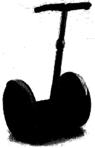
_-The wheeled pendulum model was arguably most popularized by the commercially available product, SegwayTM (refer to Figure 4), which follows a similar design scheme. The Segway uses tilt sensors, advanced gyroscope systems, and two electronic controller circuit boards to control the motion of the vehicle (Dean Kamen, 2001). Each of these aforementioned systems requires a specialized controls system for analyzing the state-space representational model of the wheeled pendulum. Steven Hassenplug, creator of the LegWay, used a different controls system method to build a two-wheeled balancing robot (refer to Figure 5). The physical vehicle for the LegWay robot was constructed using the commercially available LEGO Mindstorms robotics kit. The controls system consists of two Electro-Optical Proximity Detector (EOPD) sensors that measure the distance between a specific location on the vehicle and the ground; this provides the tilt angle information of the pendulum portion of the vehicle for the controller (Hassenplug, 2002). Using EOPD sensors eliminates the need for the conventional use of a gyroscopic component that has been utilized by the previously mentioned developers.

Figure 5: LegWay uses EOPD sensors which omit

Figure 4: Segway HT model uses a gyroscopic the need for the conventional gyroscope system

System Dynamics

In order to create a physical model, the system dynamics of the wheeled pendulum first needed to be understood. Two representations of the wheeled pendulum were analyzed to determine the model design. The equations of motion for each system were derived using free-body diagram analysis of the wheeled-portions and the pendulums for each system.

FBD Analysis 1

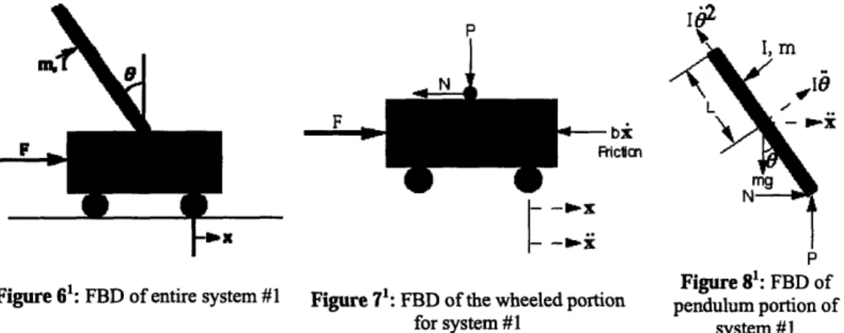
Inverted pendulum systems are typically modeled as a wheeled-cart with a rigid rod (pendulum) attached, as shown in Figures 6, 7, and 8.

Ii P .. I F

_{--- bx}

Figure

6:

system

FD

of

entire

#1

Figure 61: FBD of entire system #1 Figure 71: FBD of the wheeled portion

for system #1

Figure 81: FBD of

pendulum portion of

system #1

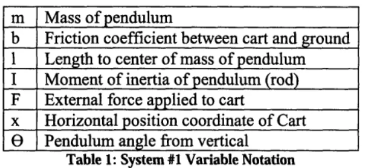
Table 1 explains the notation for each free-body diagram figure. I M I Mass of the cart

' Images were obtained from the CTM website maintained by the University of Michigan (see Reference #7).

b

m Mass of pendulum

b Friction coefficient between cart and ground 1 Length to center of mass of pendulum I Moment of inertia of pendulum (rod) F External force applied to cart

x Horizontal position coordinate of Cart

e

Using Newtonian laws, each component can be analyzed and related to form the equations of motions2 for the entire system.

Wheeled-Cart:

Mi+bi+ N- F

(1)

Pendulum:

N

m,IMl&mo-=Iae

(2)

Pai +N

-

-

nuemlI+m-i

(3)

Free-body diagram analysis yields the following equations of motion:

EOM

Entire

System:

4,

i~

iE`

-i

E--F

t

V+l

(4)

(I+mO)&+ = O- .4ueNh= (5)

Mathematical Modeling. Matlab Analysis of FBD system #1

Each FBD system was analyzed using a mathematical modeling system, MatlabTM, to observe the system behavior under variable constant parameters. Matlab scripts for analysis of FBD system #1 were modified from existing scripts found on a "Control Tutorials for Matlab" website maintained by the University of Michigan (see Reference 7). Matlab scripts for the first system were created using transfer functions and

state-2 Equations for FBD Analysis of System #2 were obtained from the CTM website maintained by the

space modeling techniques (refer to Appendix A for full Matlab scripts). Matlab analysis of the wheeled-cart inverted pendulum system showed the following results:

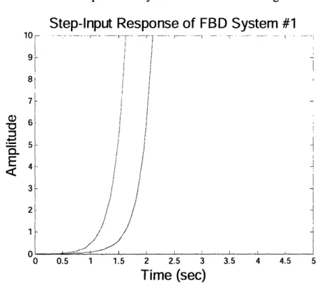
Step-Input Response of FBD System #1

10 - , - --- ---- --- --- ... ': -.----I .' i E , 5 I 9- / 0 0.5 1 1.5 2 2.5 3 3.5 4 4.5 5

Time (sec)

Figure 9: Matlab Result of Step Impulse Response for State Space Model of FBD system #1

In the above Figure 9, the cart position (in blue, on right) is shown with respect to the pendulum angle (in green, on left). As predicted, this model is unstable and requires the

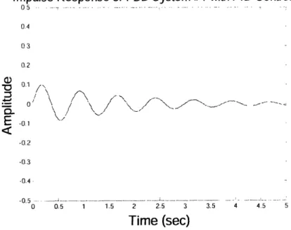
addition of a controls system. One commonly used controls system is the PID (proportional-integral-derivative) control, which can be mathematically modeled and simulated. The addition of a PID control using Matlab mathematical modeling results in system stability, as shown in Figure 10. Refer to Appendix A for full Matlab script.

Impulse Response of FBD System #1 with PID Controller 0.4 03 1.2 : 0 o.

\

\/

s

E

.

Time (sec)

Figure 10: Matlab Result of Step Impulse Response for State

system #1

Space Model with PID control for FBD

FBD Analysis 2

Analysis of the second free-body diagram of the inverted pendulum models the system as a unicycle-type design-the two masses (the wheel and the pendulum) are connected with a rigid rod (see Figures 11, 12, and 13).

X2

2

m

g

I

,ml

T

Figure 12: FBD of wheeled portion Figure 13: FBD of pendulum

for system #2 (Gossard, 2006) for system #2 (Gossard, 2006)

1

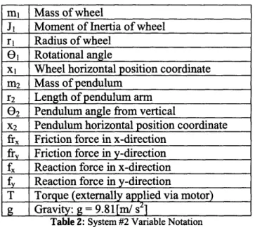
Table 2 explains the variable constants used in FBD analysis of system #2. mi Mass of wheel

J1 Moment of Inertia of wheel

r, Radius of wheel 01 Rotational angle

xl Wheel horizontal position coordinate m2 Mass of pendulum

r2 Length of pendulum arm

02 Pendulum angle from vertical

x2 Pendulum horizontal position coordinate

fr, Friction force in x-direction fr Friction force in y-direction fx Reaction force in x-direction

f

T Torque (externally applied via motor) g Gravity: g = 9.81 [m/ s2]

Table 2: System #2 Variable Notation

Isolating each component for free-body diagram analysis results in the following equations of motion3 for the wheeled-portion and the pendulum, respectively.

Wheeled-Portion:

Pendulum:

f. - f.r = mAi

T

= A.^

Kinematic Relations:

x1

Substitution and rearrangement of the above equations result in the following equations of motion for the entire system:

EOM Entire System:

(71 = _(12±B

+

I)(1

Jeq eq r2 where:

J4, = J

+ (I + Mn2)rl

3 Equations of motion for FBD analysis of system #2 were obtained from documents created by Professor David Gossard of the Mechanical Engineering department at M.I.T. (see Reference 3).

(6) (7) -

T=

r2202

mff2gr2sinO- T =

mr2

2

(13)

Mathematical Modeling: Matlab Analysis of FBD system #2

Matlab analysis was conducted on the second system using an ordinary differential equation solver function-ODE45 (refer to Appendix A for full Matlab script). Using equations of motion (12) and (13), the following results were obtained:

10 5 0

5

E

Response of FBD System #2

Time (sec)

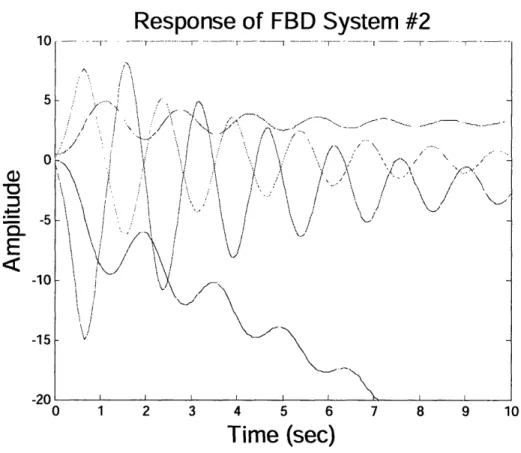
Figure 14: Matlab Result for State Space Model of FBD system #2

9 10

6=(~y~a,

-(

2)T

r2 wT~r2

--Each of the colored graphs represents the rotational and translational motions of both the wheeled and pendulum portions of the system. This response does not factor any damping effects that may be caused, for example, by air resistance. The response shows the changes in the angles from the vertical for each portion of the system: the angular velocity (blue) and angular acceleration (green) of the wheel, and the angular velocity (turquoise) and angular acceleration (red) for the pendulum. This system represents the idealized situation in the absence of damping effects, and shows the predicted cyclic motions of the wheeled pendulum system.

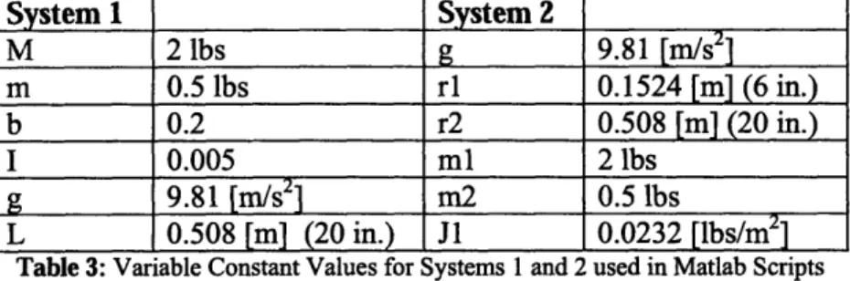
For all Matlab scripts, the following constant values were used:

System 1 System 2 M 2 lbs g 9.81 [m/s2] m 0.5 lbs rl 0.1524 [m] (6 in.) b 0.2 r2 0.508 [m] (20 in.) I 0.005 ml 2 lbs g 9.81 [m/s2] m2 0.5 lbs L 0.508 [m] (20 in.) J1 0.0232 [lbs/m2]

Table 3: Variable Constant Values for Systems 1 and 2 used in Matlab Scripts

Variable Design Factors

Based on these Matlab mathematical models, several design factors could be deduced. Two factors that can change the relative stability of the system are the masses of the pendulum head with respect to the wheel mass, and the length of the pendulum arm. Increased stability results in a longer pendulum arm length, and a smaller pendulum head mass (with respect to the wheeled system).

Design Iteration 1

Research of previously designed wheeled pendulum systems showed a design

predilection closer towards the unicycle-type design of system 2. Based on the success of these existing systems, design iteration 1 followed a similar design schema.

Figure 15: Design Iteration 1

Pendulum Portion

The main design consideration of the wheeled pendulum system is the housing for the electrical components of the controls system. With the unicycle-type design, the controls mechanisms needed to be placed along the pendulum arm portion of the physical vehicle. The main focus of this design iteration was to completely protect the fragile parts of the controls system by keeping all electrical components housed within the aluminum rectangular tube. Two sliding entrances would allow access to the controls system on either side of the tubing. The use of aluminum material would provide robust protection

against damage due to forceful impact. Figure 16 shows the primary module for design

iteration 1.

Figure 16: Pendulum Arm Module for Design Iteration I

Wheeled Portion

The wheeled portion of the inverted pendulum would be comprised of two six inch diameter plastic wheels, two DC motors, and the bearings and couplings used to link the wheels and motors together (Refer to Figure 17).

Figure 17: Wheeled Portion of Inverted Pendulum for all design iterations

Each of the wheels would be press-fit onto an axle shaft and placed through a bearing. The shaft would be powered by the motor through a coupling component. 3-D models and diagrams can be found in Appendix B.

Design Complications and Considerations

Preliminary sketch models of design iteration 1 using foam-core material showed several flaws in this design. Although the housing portion of the pendulum arm provided ample protection against damage, the sliding portions only allows access to fifty percent of the total space inside, rendering the other fifty percent completely useless. Since the design specifications of the controls system are currently unknown, the limited spatial allowance could cause this entire design vehicle to be unusable. Anticipated problems with the

controls system also made up a large factor in changing the design- while protection against damage is an important design consideration, ease of access to the controls system is more crucial.

Design Iteration 2

Due to the limited access in design iteration 1, the main concern behind design iteration 2 was to create a strong casing for the electrical components, but also allow for ease of access in order to modify the controls system. The most efficient way to modify the controls system would be to allow for the entire system to be exposed. Design iteration 2 is therefore able to be fully disassembled if necessary.

Figure 18: Design Iteration 2

Pendulum Portion

The use of rectangular tubing as the outer-most casing ensures minimal damage to the inner components of the pendulum arm. Figure 19 shows the main module component for design iteration 2.

Figure 19: Pendulum-Arm Module for Design Iteration 2

Unlike design iteration 1, this design allows for complete access to the controls system, and allows visibility of the controls system at all times to the user. The use of the rectangular tubing also allows for variability of the pendulum arm length and width. Multiple base-plate templates for the extrusions could be manufactured to create varied sizes of the pendulum depending on the controls system specifications. The extrusions would provide robust protection against any damage due to mishandling, since the controls system would be attached to the aluminum plate completely encased within the four extrusions. Ability to fully disassemble the pendulum arm portion will be useful if extensive modification or repair needs to be conducted on the controls system.

The wheeled portion of design iteration 2 remains the same as in design iteration 1 since no major flaws were found in the first design concept (refer to Figure 17).

Design Complications and Considerations

Although design iteration 2 solves both problems concerning robustness and

accessibility, several modifications could be further made to improve the design of the prototyped vehicle. For its purpose as an experimental vehicle to be used in the laboratory component of the 2.004 course, the wheeled pendulum prototype does not need to have all four extrusions as a protective casing. Two aluminum extrusions would provide ample protection against the predicted damage of rough-handed use. The fabrication of base-plate templates to create variable width and length is also somewhat extraneous, since the height of the extrusions should provide ample space to house the entire controls system. Also, ease of manufacturing base-plate templates would be inefficient for the purpose of this prototype vehicle.

Design Iteration 3

Design iteration 3 was modified to cut-out the unnecessary components of design iteration 2. Figure 20 illustrates the major changes made.

Figure 20: Design Iteration 3

Pendulum Portion

Design iteration 3 uses only two aluminum extrusions to house the controls system and eliminates the use of the aluminum plate to hold the electrical components-- circuit boards, and other parts can be attached directly to the extrusion casing. The extrusions would be attached to two aluminum pieces that can be disassembled at both ends from

the wheeled-portion, and the pendulum-head portion of the vehicle. Figure 21 shows the detached pendulum-arm module for design iteration 3.

Figure 21: Pendulum-Arm Module for Design Iteration 3

The two aluminum extrusions will still provide ample protection against impact damage. The detachable pendulum-arm portion will allow for ease of access for modifications to the controls system. Attaching the electrical components directly to the extrusions also eliminates any extra weight from the aluminum used in design iteration 2.

The wheeled portion of design iteration 3 remains the same as in design iteration 1 since no major flaws were found in the first design concept (refer to Figure 17).

Prototype

Materials Selection

Aluminum was used to create the prototype vehicle of design iteration 3 since it is robust enough to provide protection to the controls system components of the inverted

pendulum. Of the readily available materials, aluminum was also the most cost-efficient material to use to create the first prototype of this design. Table 4 discusses the necessary materials for design iteration 3.

Type of Aluminum Amount

1 "x 1" square extrusions (for pendulum arm and bearings) 46"

1/4"

thick

1/8" thick sheet 20" x 20"

3/4" diameter rod (for press-fit wheel shaft) 6"

Extraneous Materials

6" diameter, polypropylene wheels 2

Table 4: Materials Needed for Design Iteration 3 Prototype

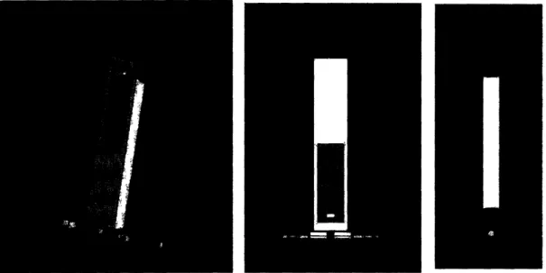
Figure 22 shows the prototype frame of the wheeled portion, pendulum arm, and

Figure 22: Prototype Frame of Inverted Pendulum

Wheeled Portion

The wheeled portion of the inverted pendulum uses two 6" diameter polypropylene wheels, which are press-fit onto manufactured axle shafts (refer to Figure 23).

Figure 24: Manufactured Axle Shaft for Wheel

The axles are placed through bearings (refer to Figures 24 and 25) and connected to a DC motor using a coupling.

Figure 25: Bearing for Axle Shaft Figure 26: Axle Shaft and Bearing

Exact dimensions and models of each of the base components can be found in Appendix B. Additional images of the physical prototype can be found in Appendix C.

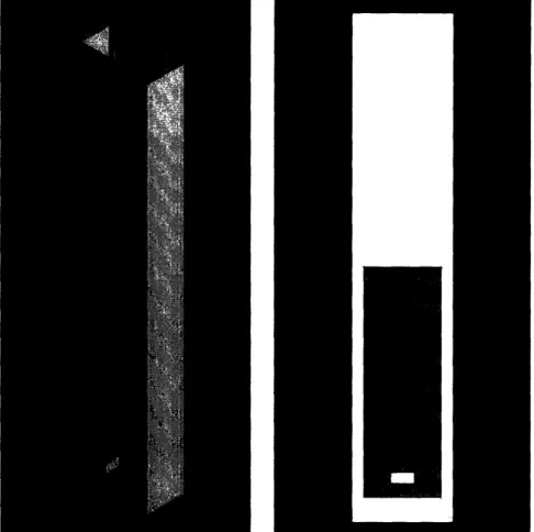
Pendulum Arm

The pendulum arm was created by welding both aluminum extrusions to two aluminum rectangular base-pieces (refer to Figure 26).

Figure 27: Pendulum Arm portion of Inverted Pendulum

Dimensions and solid models for the pendulum arm component can be found in Appendix B.

Pendulum Head

Because the specific components of the controls system are currently unknown, the pendulum head was designed to house several possible parts, such as the batteries for the system and the processing board (refer to Figure 27).

Two circular aluminum pieces will be attached to the base of the head to add aesthetics to the system and create a more accurate pendulum design. Part drawings for the pendulum head can also be found in Appendix B. Additional images of the prototype can be found in Appendix C.

Each of the three components that make up the prototype can be disassembled from one another. The three portions are attached using #8-32 and #10-32 nuts and bolts of varying lengths.

Future Work

Due to a time constraint, I was unable to start producing the controls system for the wheeled-pendulum robot. An understanding of the necessary electrical components required of the controls system would have allowed for a more precise prototype design, and would also have helped determine the weight distribution of the system. Matlab analysis of the inverted pendulum system showed that stability is dependant on the mass of both the wheeled-portion and the pendulum. Since estimated values were used to determine the parameters of the system, implementing a physical controls system would have allowed for a second, more accurate prototype to be created based on the additional mass a controls system would cause. Without the controls component, the stability of the current prototype is questionable, since Matlab modeling was also based on ideal

References

1. Anderson, D.P, 'Nbot, a two wheel balancing robot', Viewed 6 March 2006 <http://www.geology.smu.edu/-dpa-www/robo/nbot>

2. Feng, Qing; Yamafuji, Kazuo, 'Design and simulation of control systems of an inverted pendulum', Robotica. Vol. 6, no. 3, pp. 235-241. 1988

3. Gossard, David, 2006, '2.004 System Dynamics and Control, Wheeled Pendulum' 4. Grasser, Felix, Alonso D'Arrigo, Silvio Colombi & Alfred C. Rufer, 2002, 'JOE:

A Mobile, Inverted Pendulum', IEEE Transactions on Industrial Electronics, vol 49.

<http://leiwww.epfl.ch/publications/grasser darrigo_colombi_rufermic_01 .pdf> 5. Hassenplug, Steve, 2002, 'Steve's Legway', Viewed 6 March 2006

<http ://www.teamhassenplug.org/robots/legway/>

6. Kamen, Dean, 2001, Viewed 6 March 2006, http://www.segwa.com

7. University of Michigan, 1997, 'Controls Tutorials for Matlab,' Viewed 15 March 2006. <http://www.engin.umich.edu/group/ctm/index.html>

Appendix A: Matlab Scripts for FBD Analysis

% MATLAB SCRIPT FOR FBD ANALYSIS OF INVERTED PENDULUM SYSTEM #1 %Approximated Values for Variables

M = 2.; % in lbs (mass of wheeled portion) m = 0.5; % in lbs (mass of pendulum portion) b = 0.2; % friction coefficient

i = 0.005; % moment of inertia g = 9.8; % gravity in m/sA2

1 = 0.508; % in [ml length (= 20 inches)

%State-Space Model Representation (Matrix Form)

A =[0 1 0 0; 0 -(i+m*l^2)*b/(i*(M+m)+M*m*A12) (m^2*g*1^2)/(i*(M+m)+M*m*1^2) 0; 0 0 0 1; 0 -(m*l*b)/(i*(M+m)+M*m*l^2) m*g*l*(M+m)/(i*(M+m)+M*m*1A2) 0] B= [ 0; (i+m*1^2)/(i* (M+m)+M*m*1^2); 0; m*l/(i*(M+m)+M*m*1^2)] C = [1 0 0 0; 0 0 1 0] D= [0; 0] T=0:0.05:10; U=0.2*ones(size(T)); [Y,X]=lsim(A,B,C,D,U,T); plot (T,Y) xlabel('Time (sec)','FontSize',16) ylabel('Amplitude','FontSize',16)

title('Step-Input Response of FBD System #1','FontSize',16)

axis([0 5 0 100])

% MATLAB SCRIPT FOR FBD ANALYSIS OF INVERTED PENDULUM SYSTEM #1 WITH PID

% CONTROLLER

%Approximated Values for Variables

M = 2.; % in lbs (mass of wheeled portion) m = 0.5; % in lbs (mass of pendulum portion) b = 0.2; % friction coefficient

i = 0.005; % moment of inertia g = 9.8; % gravity in m/s^2

1 = 0.508; % in [m] length (= 20 inches) num = [m*l/((M+m)*(i+m*l^2)-(m*l)^2) 0] den = [1 b*(i+m*1^2)/((M+m)*(i+m*lA2)-(m*l)^2) -(M+m)*m*g*l/((M+m)*(i+m*lA2)-(m*l)^2) -b*m*g*l/((M+m)*(i+m*l^2)-(m*l) 2)] kd = 1; k = 100; ki = 1; numPID = [kd k ki]; denPID = [1 0]; numc = conv(num,denPID) denc = polyadd(conv(denPID,den),conv(numPID,num)) t=0:0.01:5;

impulse (numc, denc, t)

axis([0, 5, -0.5, 0.5])

xlabel('Time','FontSize',16) ylabel('Amplitude','FontSize',16)

title('Impulse Response of FBD System #1 with PID Controller', 'FontSize',14)

%POLYADD FUNCTION SCRIPT FOR SYSTEM #1 function[poly]=polyadd(polyl,poly2) %Copyright 1996 Justin Shriver

%polyadd(polyl,poly2) adds two polynominals possibly of uneven length if length(polyl)<length(poly2) short=polyl; long=poly2; else short=poly2; long=polyl; end mz=length(long)-length(short); if mz>0 poly=[zeros(l,mz),short]+long; else poly=long+short; end

% MATLAB SCRIPT FOR FBD ANALYSIS OF INVERTED PENDULUM SYSTEM #2 dy = zeros(4,1)

[t,y] = ode45(@whipeqnsl, [0 10], [0, 0, 0.5, 0]);

xlabel('Time (sec)','FontSize',16) ylabel( 'Amplitude', 'FontSize',16)

title('Response of FBD System #2','FontSize',16)

axis([0 10 -20 10])

% MATLAB SCRIPT FOR FBD ANALYSIS OF INVERTED PENDULUM SYSTEM #2 (whipseqnsl function script)

function dy = whipeqnsl(t,y)

% Approximated Values for Variables

g = 9.81; %[m/s^2] rl = 0.1524.; %in [m], = 6 inches r2 = 0.508.; % in [m], = 20 inches ml = 2.; % in lbs m2 = 0.5; %in lbs, J1 = 0.5*ml*(rl^2).; % 0.0232 in lb*in^2

%Moment of Inertia: Solid Cylinder=1/2*M*R^2, Hollow Cylinder= %l1/2*M*(Ri^2+Ro^2) Jeq = J1 + (ml + m2)*rl^2; Jeq = J1; dy = zeros(4,1); dy(l) = y(2); dy(2) = -(m2*rl*g/Jeq)*sin(y(3)); dy(3) = y(4);

Appendix B: Design Iteration Part Drawings (SolidWorks)

Appendix Figure 1: SolidWorks Part Drawing for Wheeled Portion of Inverted Pendulum Prototype ... 37 Appendix Figure 2: SolidWorks Part Drawings for Components of Wheeled Portion .... 38 Appendix Figure 3: SolidWorks Part Drawing for Design Iteration 1 Pendulum Arm .... 39 Appendix Figure 4: SolidWorks Part Drawing for Design Iteration 2 Pendulum Arm .... 40 Appendix Figure 5: SolidWorks Part Drawing for Design Iteration 3 Pendulum Arm .... 41 Appendix Figure 6: SolidWorks Part Drawing for Pendulum Head of Inverted Pendulum Prototype ... 42

. . ... . .. a _ | V|. . .. U I '... ~,..l'.llnl ·

~

I

1.

Appendix Figure 1: SolidWorks Part Drawing for Wheeled Portion of Inverted Pendulum Prototype II II- -I I I C0 1a' e= Du-l:

05

0

0.3$

.w ttii*i' 4P lilw fmlillg_{>.~w @F I~ oICP}

a*M O^Fr~vr~~~ A||~e~km e^WFrr tAIn Mi i

0

0

0

-6

. ._ .. . A..W....

W"IWC

I

I

'I0~~~~.-1

I

-IL

Appendix Figure 3: SolidWorks Part Drawing for Design Iteration I Pendulum Arm

I- And X Y . I J1 .n a--, I 1-1 4O i Ij

_-I:I so . .I L ¶W MW6'MWII. 'ilt I IkSi, - Iv . WLWinc m4c~; 4~ tI o.1 C4 I .i I 0

-

0,60

!-- to-a.-

*4CL

Cot.

-I

Appendix Figure 4: SolidWorks Part Drawing for Design Iteration 2 Pendulum Arm

IIIIIIII_______UWYI··llllll·-·U--·l· ·I--L-Y--·Y---··-·II·C-.---__···IYI· _·__I_...·1_111..-· II

- enS s S - -i m l / m l /' l I l- I k*..! lmd - _l ' E_ l - --- 4 l- .. i . rr o-i -E _ .; s .... .. ,, ,,,, ... _ b " rI + .... ... _. _ _ _ _ _ __ ___ _ -- !y _ LI -II · . v . ,nd.-1· * _ . ·II A-M I- 1-.... L r I I I I I A... ARIOCH

~m lmma mI. l~mmpb M-WIT r F F o4 e aK4dLia_~ --F , 'utwAJU Im om.

AIL"--I,

[

*pnd ulumrmarO |

Appendix Figure 5: SolidWorks Part Drawing for Design Iteration 3 Pendulum Arm

II__IUII___I*IUI__I-·-yll·-···ll 11.1111--- _111111^..1_^_1·1 __ ^._·_.i __ _ s __ i- -- -- - -I - I _, |- -§ - § --2 _ I _ 1 I - __ * ,# I -- ---- --- .. . . ._r --F' #8F --- M.l -_.- -- - ---- -- - . . I ---· . h. I I I m. ' i I _ m I I

i 0

0

0

0,i

1.

n

l

I 4F

-

%

;AMO OAU HO E U' 4* U .Ul,&A

I '- I -.. I *l.i I ui' -".l I -" I I1 i. ,hlI. Ar MA Lfop Aemb 1"5 ..-- , r- I,- ... InhSl', IU Ie. 1 l-1,N in.l 3 ,MN Z

Appendix Figure 6: SolidWorks Part Drawing for Pendulum Head of Inverted Pendulum Prototype

YU_I__IIWI_·__L______IYYIY·- YI--X--·-·- IIIIIXI---.· I-· -Illl--X II.- I·-^I

- m 1 s :. . '· Z i- . -- -- I . _ ... . * - .-·'~~~~~~~~~~~~~~~~~~~~~~~~~~~~~~~~~~~~~^ .... ...

I

Appendix: C: Prototype Images

Pendulum Arm:

MITLibraries

http://libraries. mit. edu/docs

DISCLAIMER OF

QUALITY

Due to the condition of the original material, there are unavoidable

flaws in this reproduction. We have made every effort possible to

provide you with the best copy available. If you are dissatisfied with

this product and find it unusable, please contact Document Services as

soon as possible.

Thank you.

Some pages in the original document contain pictures,

graphics, or text that is illegible.