Complete VLSI implementation of improved low complexity chase Reed-Solomon decoders

Complete VLSI Implementation of Improved Low

Complexity Chase Reed-Solomon Decoders

by

Wei An

B.S., Shanghai Jiao Tong University (1993)

M.S., University of Delaware (2000)

MASSACHUSETTS INSTITUTE

OF TECHNOLOGY

OCT

3

5 2010

LIBRARIES

Submitted to the Department of Electrical Engineering and Computer

Science

in partial fulfillment of the requirements for the degree of

Electrical Engineer

at the

MASSACHUSETTS INSTITUTE OF TECHNOLOGY

ARCHVES

September 2010

@

Massachusetts Institute of Technology 2010. All rights reserved.

Author .

Department

Certified by...

of Electrical Engmeering and Computer Science

' September 3, 2010

//

U

/

Vladimir M. Stojanovid

Associate Professor

Thesis Supervisor

Accepted by...

Terry P. Orlando

Chairman, Department Committee on Graduate Theses

Complete VLSI Implementation of Improved Low

Complexity Chase Reed-Solomon Decoders

by

Wei An

Submitted to the Department of Electrical Engineering and Computer Science on September 3, 2010, in partial fulfillment of the

requirements for the degree of Electrical Engineer

Abstract

This thesis presents a complete VLSI design of improved low complexity chase (LCC) decoders for Reed-Solomon (RS) codes. This is the first attempt in published research that implements LCC decoders at the circuit level.

Based on the joint algorithm research with University of Hawaii, we propose sev-eral new techniques for complexity reduction in LCC decoders and apply them in the VLSI design for RS [255, 239,17] (LCC255) and RS [31, 25, 7] (LCC31) codes. The major algorithm improvement is that the interpolation is performed over a subset of test vectors to avoid redundant decoding. Also the factorization formula is reshaped to avoid large computation complexity overlooked in previous research. To maintain the effectiveness of algorithm improvements, we find it necessary to adopt the system-atic message encoding, instead of the evaluation-map encoding used in the previous work on interpolation decoders.

The LCC255 and LCC31 decoders are both implemented in 90nm CMOS process with the areas of 1.01mm2 _{and 0.255mm}2 _{respectively. Simulations show that with} 1.2V supply voltage they can achieve the energy efficiencies of 67pJ/bit and 34pJ/bit at the maximum throughputs of 2.5Gbps and 1.3Gbps respectively. The proposed algorithm changes, combined with optimized macro- and micro-architectures, result in a 70% complexity reduction (measured with gate count). This new LCC design also achieves 17x better energy-efficiency than a standard Chase decoder (projected from the most recent reported Reed Solomon decoder implementation) for equivalent area, latency and throughput. The comparison of the two decoders links the significantly higher decoding energy cost to the better decoding performance. We quantitatively compute the cost of the decoding gain as the adjusted area of LCC255 being 7.5 times more than LCC31.

Thesis Supervisor: Vladimir M. Stojanovid Title: Associate Professor

Acknowledgments

I want to thank Dr. Fabian Lim and Professor Aleksandar Kavoid from University of

Hawaii at Manoa for the cooperation on the algorithm investigation. I also want to thank Professor Vladimir Stojanovid for his inspiring supervision. Finally, I want to acknowledge Analog Devices, Inc. for supporting my study at MIT.

Contents

1 Introduction

1.1 Reed-Solomon codes for forward error correction . . . . 1.2 Low complexity Chase decoders for RS codes . . . .

1.3 Major contributions and thesis topics . . . .

2 Background

2.1 Encoders and HDD decoders for Reed-Solomon codes . . . . 2.2 Channel model, signal-to-noise ratio and reliability . . . . 2.3 The LCC decoding algorithm . . . .

3 Algorithm Refinements and Improvements

3.1 Test vector selection . . . .

3.2 Reshaping of the factorization formula . . . .

3.3 Systematic message encoding . . . .

4 VLSI Design of LCC Decoders

4.1 Digital signal resolution and C++ 4.2 Basic Galois field operations 4.3 System level considerations . . . .

4.4 Pre-interpolation processing . . . 4.4.1 Stage I . . . . 4.4.2 Stage II . . . . 4.4.3 Stage III . . . . simulation 13 13 15 16 19 19 22 23 29 29 32 32 35 . . . . 35 . . . . 37 . . . . 39 . . . . 40 . . . . 41 . . . . 43 . . . . 44

4.5 Interpolation . . . .

4.5.1 The interpolation unit . . . . 4.5.2 The allocation of interpolation units . . . . 4.5.3 Design techniques for interpolation stages . . . 4.6 The RCF algorithm and error locations . . . . 4.7 Factorization and codeword recovery . . . . 4.8 Configuration module . . . .

5 Design Results and Analysis

5.1 Complexity distribution of LCC design . . . . 5.2 Comparison to standard Chase decoder based on HDD

5.3 Comparison to previous LCC work . . . .

5.4 Comparison of LCC255 to LCC31 . . . .

6 Conclusion and Future Work

6.1 C onclusion . . . .

6.2 Future work . . . .

A Design Properties and Their Relationship

B Supply Voltage Scaling and Process Technology Transformation C I/O interface and the chip design issues

D Physical Design and Verification

D.1 Register file and SRAM generation . . . . D.2 Synthesis, place and route . . . . D.3 LVS and DRC design verification . . . .

D.4 Parasitic extraction and simulation . . . .

. . . . 44 . . . . 44 . . . . 46 . . . . 50 . . . . 52 . . . . 55 . . . . 57 59 . . . . 60 . . . . 64 . . . . 66 . . . . 67 73 73 74 75 77 81 85 85 85 90 93

List of Figures

3-1 Simple rj = 3 example to illustrate the difference between the standard

Chase and Tokushige et. al. [30] test vector sets. The standard Chase test vector set has size 27 = 8. The Tokushige test vector set covers a

similar region as the Chase, however with only h = 4 test vectors. . . 30

3-2 Performance of test vector selection method for RS[255, 239,17]. . . . 31

4-1 Comparison of fixed-point data types for RS[255, 239, 17] LCC decoder. 36 4-2 Galois field adder . . . . 37

4-3 The XTime function . . . . 38

4-4 Galois field multiplier . . . . 38

4-5 Horner Scheme . . . . 39

4-6 Multiplication and Division of Galois Field Polynomials . . . . 39

4-7 VLSI implementation diagram. . . . . 40

4-8 Data and reliability construction . . . . 41

4-9 Sort by the reliability metric . . . . 42

4-10 Compute the error locator polynomial . . . . 43

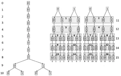
4-11 Direct and piggyback approaches for interpolation architecture design. 45 4-12 The Interpolation Unit. . . . . 47 4-13 Tree representation of the (full) test vector set (2.12) for LCC255

de-coders, when 71 = 8 (i.e. size 28). The tree root starts from the first

point outside

J

4-14 Sub-tree representation of the h = 16 fixed paths, chosen using the

4-15 Step 2 interpolation time line in the order of the sequence of group

ID's for the depth-first and breadth-first approaches . . . . 49

4-16 Sub-tree representation of the h = 4 fixed paths for RS [31, 25, 7 decoder. 50 4-17 RCF block micro-architecture. . . . . 53

4-18 Implementation diagram of the RCF algorithm. . . . . 54

4-19 Diagram for root collection. . . . . 55

4-20 Detailed implementation diagram of Stage VII. . . . . 56

5-1 The circuit layout of the LCC design . . . . 60

5-2 Complexity distribution v.s. number of test vectors h . . . . 64

5-3 Decoding energy cost v.s. maximum throughput with supply voltage ranging from 0.6V to 1.8V . . . . 69

5-4 Decoding energy cost v.s. adjusted area with constant throughput and latency as the supply voltage scales from 0.6V to 1.8V . . . . 70

5-5 Decoding energy cost v.s. adjusted area with equivalent/constant throughput and latency as the supply voltage scales from 0.6V to 1.8V 71 C-1 The chip design diagram . . . . 83

D-1 ASIC Design Flow. . . . . 86

D-2 Floorplan of the LCC255 decoder . . . . 89

D-3 Floorplan of the LCC31 decoder . . . . 90

D-4 Floorplan of the I/O interface . . . . 91

List of Tables

5.1 Implementation results for the proposed LCC VLSI design . . . . 60

5.2 Gate count of the synthesized LCC decoder . . . . 62

5.3 Complexity Distribution of the synthesized LCC decoder . . . . 63

5.4 Comparison of the proposed LCC with HDD RS decoder and the cor-responding standard Chase decoder . . . . 66

5.5 Area adjustment for comparison of decoding energy-costs . . . . 67

5.6 Multiplier usage in the proposed LCC decoder . . . . 68

5.7 RAM usage in the proposed LCC decoder . . . . 68

5.8 Comparison of the proposed LCC architecture and the work in [33] . 68 5.9 Computed limits of clock frequency and adjusted area along with through-put and latency for LCC31 and LCC255 . . . . 71

C.1 Number of Bits of Decoder Interface . . . . 81

C.2 The I/O interface to the outside environment . . . . 83

D.1 Memory usage in the chip design . . . . 87

D.2 Physical parameters of the circuit layout . . . . 93

Chapter 1

Introduction

In this thesis, we improve and implement the low complexity chase (LCC) decoders for Reed-Solomon (RS) codes. The complete VLSI design is the first effort in published research for LCC decoders. In this chapter, we briefly review the history of Reed-Solomon codes and LCC algorithms. Then we outline the contributions and the organization of the thesis.

1.1

Reed-Solomon codes for forward error

correc-tion

In data transmission, noisy channels often introduce errors in received information bits. Forward Error Correction (FEC) is a method that is often used to enhance the reliability of data transmission. In general, an encoder on the transmission side trans-forms message vectors into codewords by introducing a certain amount of redundancy and enlarging the distance'between codewords. On the receiver side, a contaminated codeword, namely the senseword, is processed by a decoder that attempts to detect and correct errors in its procedure of recovering the message bits.

Reed-Solomon (RS) codes are a type of algebraic FEC codes that were introduced

by Irving S. Reed and Gustave Solomon in 1960 [27]. They have found widespread 'There are various types of distance defined between codeword vectors. See [23] for details.

applications in data storage and communications due to their simple decoding and their capability to correct bursts of errors [23]. The decoding algorithm for RS codes was first derived by Peterson [26]. Later Berlekamp [3] and Massey [25] simplified the algorithm by showing that the decoding problem is equivalent to finding the shortest linear feedback shift register that generates a given sequence. The algorithm is named after them as the Berlekamp-Massey algorithm (BMA) [23]. Since the invention of the BMA, much work has been done on the development of RS hard-decision decoding (HDD) algorithms. The most notable work is the application of the Euclid Algorithm [29] for the determination of the error-locator polynomial. Berlekamp and Welch [4] developed an algorithm (the Berlekamp-Welch(B-W) algorithm) that avoids the syndrome computation, the first step required in all previously proposed decoding algorithms. All these algorithms, in spite of their various features, can correct the number of errors up to half the minimum distance dmin of codewords. There had been no improvement on decoding performance for over 45 years since the introduction of

RS codes.

In 1997, a breakthrough by Sudan made it possible to correct more errors than previous algebraic decoders [28]. A bivariate polynomial Q(X, Y) is interpolated over the senseword. The result is shown to contain, in its y-linear factors, all codewords within a decoding radius t > dmin/2. The complexity of the algorithm, however,

increases exponentially with the achievable decoding radius t. Sudan's work renewed research interest in this area, yielding new RS decoders such as the Guruswarmi-Sudan algorithm [9], the bit-level generalized minimum distance (GMD) decoder [12], and the Koetter-Vardy algorithm [16].

The Koetter-Vardy algorithm generalizes Sudan's work by assigning multiplicities to interpolation points. The assignment is based on the received symbol reliabili-ties [16]. It relaxes Sudan's constraint of passing Q(x, y) through all received values with equal multiplicity and results in a decoding performance significantly surpass-ing the Guruswarmi-Sudan algorithm with comparable decodsurpass-ing complexity. Still, the complexity of the Koetter-Vardy algorithm quickly increases as the multiplicities increase. Extensive work has been done to reduce core component complexity of the

Sudan algorithm based decoders, namely interpolation and factorization [7, 15, 24]. Many decoder architectures have been proposed, e.g. [1, 13]. However, the Koetter-Vardy algorithm still remains un-implementable from a practical standpoint.

1.2

Low complexity Chase decoders for RS codes

In 1972, Chase [6] developed a decoding architecture, non-specific to the type of code, which increases the performance of any existing HDD algorithms. Unlike the Sudan-like algorithms, which enhance the decoding performance via a fundamentally different approach from the HDD procedure, the Chase decoder achieves the en-hancement by applying multiple HDD decoders to a set of test vectors. In traditional HDD, a senseword is obtained via the maximum a-posteriori probability (MAP) hard-decision over the observed channel outputs. In Chase decoders, however, a test-set of hard-decision vectors are constructed based on the reliability information. Each of such test vectors is individually decoded by an HDD decoder. Among successfully decoded test vectors, the decoding result of the test vector of highest a-posteriori

probability is selected as the final decoding result. Clearly, the performance increase

achieved by the Chase decoder comes at the expense of multiple HDD decoders with the complexity proportional to the number of involved test vectors. To construct the test-set, q least reliable locations are determined and vectors with all possible symbols in these locations are considered. Consequently, the number of test vectors and the complexity of Chase-decoding increase exponentially with q.

Bellorado and Kavoid [2] showed that the Sudan algorithm can be used to im-plement Chase decoding for RS codes, however, with decreased complexity. Hence the strategy is termed the low complexity Chase (LCC), as opposed to the standard

Chase. In the LCC, all interpolations are limited to a multiplicity of one. Application

of the coordinate transformation technique [8, 17] significantly reduces the number of interpolation points. In addition, the reduced complexity factorization (RCF) tech-nique proposed by Bellorado and Kavoid, further reduces the decoder complexity, by selecting only a single interpolated polynomial for factorization [2]. The LCC has

been shown to achieve performance comparable to Koetter-Vardy algorithm, however at lower complexity.

Recently, a number of architectures have been proposed for the critical LCC blocks, such as backward interpolation [15] and factorization elimination [14], [33].

However, a full VLSI micro-architecture and circuit level implementation of the LCC algorithm still remains to be investigated. This is the initial motivation of the research presented in the thesis.

1.3

Major contributions and thesis topics

This thesis presents the first2_{, complete VLSI implementation of LCC decoders. The} project follows the design philosophy that unifies multiple design levels such as al-gorithm, system architecture and device components. Through the implementation-driven system design, algorithms are first modified to significantly improve the hard-ware efficiency. As the result of the joint research of MIT and University of Hawaii, the main algorithm improvements include test vector selection, reshaping of the fac-torization formula and the adoption of systematic encoding.

Two decoders, LCC255 and LCC31 (for RS [255, 239,17] and RS [31, 25, 7] codes respectively), are designed with Verilog HDL language. Significant amount of effort is devoted to the optimization of the macro- and micro architectures and various cycle saving techniques are proposed for the optimization of each pipeline stages. While being optimized, each component is designed with the maximal flexibility so they can be easily adapted to meet new specifications. The component flexibility greatly supports the design of two LCC decoders simultaneously.

The Verilog design is synthesized, placed-and-routed and verified in a represen-tative 90nm CMOS technology. The physical implementation goes throughput com-prehensive verifications and is ready for tape-out. We obtain the power and timing estimation of each decoder by performing simulations on the netlist with parasitics

2In _{previously published literature (e.g. [15] and [14]), the described LCC architecture designs}

extracted from the circuit layout. The measurements from the implementation and simulations provide data for comprehensive analysis on several aspects of the design, such as system complexity distribution and reduction, decoding energy-cost of LCC compared to Standard Chase and comparison between LCC255 and LCC31 decoders.

The thesis topics are arranged as follows.

Chapter 2 exposes the background of LCC and the previous techniques for com-plexity reduction.

Chapter 3 presents new algorithm and architecture proposals that are essential for further complexity reduction and efficient hardware implementation.

Chapter 4 presents in detail the VLSI hardware design of LCC255 and LCC31 decoders along with macro- and micro-architecture optimization techniques.

Chapter 5 presents the comprehensive analysis on complexity distribution of the new LCC design and its comparisons to the standard Chase decoder and previous designs of LCC decoders. Comparison is also performed between LCC255 and LCC31.

Chapter 2

Background

2.1

Encoders and HDD decoders for Reed-Solomon

codes

Reed-Solomon (RS) codes are a type of block codes optimal in terms of Hamming dis-tance. An [N, K] RS code C, is a non-binary block code of length N and dimension K

with a minimum distance dmin = N - K +1. Each codeword c = [co, c, ... , cN-1]T E

C, has non-binary symbols ci obtained from a Galois field F2., i.e. ci E F23. A

primitive element of F2. is denoted a. The message m = [imo, m1, - , mK-1 ]T that needs to be encoded, is represented here as a K-dimensional vector in the Galois field F28. The message vector can also be represented as a polynomial m(x) =

mo + mix + -- -mK-1xK-1, known as the message polynomial. In encoding

pro-cess, a message polynomial is transformed into a codeword polynomial denoted as c(x) = co + cix + cN-xN

Definition 1. A message m = [n, rn1,- , mK]T is encoded to an RS codeword

c E C, via evaluation-map encoding, by i) forming the polynomial 0(x) = mo + mx+- --mK-1XK-1 , ii) evaluating 0(x) at all N = 2'- 1 non-zero elements at E F2",

z. e. ,

for all i E (,1, - , N - 1}.

In applications, a message is often encoded in a systematic format, in which the codeword is formed by adding parity elements to the message vector. This type of encoder is defined below,

Definition 2. In systematic encoding, the codeword polynomial c(x) is obtained

systematically by,

c(x) = m(x)x(N-K) + mod(m(x)x(N-K) I g)) (2.2)

where mod() is the modular operation in polynomials and g(x) =| H ₁-K)(X +

&)

the generator polynomial of the codeword space C.

An HDD RS decoder can detect and correct v < (N-K)/2 errors when recovering the message vector from a received senseword. The decoding procedure is briefly described below. Details can be found in [23].

In the first step, a syndrome polynomial S(x) = So + Six + - SN-K-1X N-K-1 is produced with its coefficients (the syndromes) computed as,

Si=r(o ), for 1 <i<N-K, (2.3)

where r(x) = ro +riX+- - -rN-1zN-1 is a polynomial constructed from the senseword. Denote the error locators Xk = aik and error values Ek = eik respectively for k =

1, 2,... , V, and ik is the index of a contaminated element in the senseword. The error

locator polynomial is constructed as,

A(x) = 1J(1 - XXk) = _{1 + Aix +Ax+} ... + Axv, (2.4)

k=1

The relation between the syndrome polynomial and the error locator polynomial is,

where 8(x) contains all non-zero coefficients with orders higher than 2t and 1(x) is named error evaluator polynomial, which will be used later for the computation of error values.

Each coefficient of A(x)S(x) is the sum-product of coefficients from S(x) and 1(x) respectively. It is noted that the coefficients between order v and 2t in A(x)S(x) are all zeros. These zero coefficients can be used to find the relation between the coefficients of S(x) and 1(x).

The relation is expressed as,

S1 S2 ... Su AV -Sv+1

S2 S3 -. Sv+1 A-1 -Sv+2(26)

Sv Sv+1 -.. S2v-1 A₁ -S2v

It is observed from (2.6) that with 2v = N - K syndromes, at most v errors can be detected. To obtain the error locator polynomial, it requires intensive computations if

(2.6) (the key equation) is solved directly. A number of efficient algorithms have been

proposed to compute the error locator polynomial, such as the Berlekamp-Massey algorithm and the Euclidean algorithm. Details of these algorithms can be found in many texts such as [23].

Chien search is commonly used to find the roots (the error locators) of the error locator polynomial. Basically, the algorithm evaluates the polynomial over the entire finite field in searching for the locations of errors. Finally, Forney algorithm is an efficient way to compute the error values at the detected locations. The formula is quoted below,

r7(X)

Ek= k) 0<k<v (2.7)

The four blocks, i.e. syndrome calculation, key equation solver, Chien search and Forney algorithm are the main components of an HDD RS decoder. The simple and efficient implementation together with the multi-error detection and correction

capability make Reed-Solomon codes commonly used FEC codes.

2.2

Channel model, signal-to-noise ratio and

reli-ability

The additive white Gaussian noise (AWGN) channel model is widely used to test channel coding performance. To communicate a message m across an AWGN channel, a desired codeword c = [co, ci, ... , cN-1 T (which conveys the message m) is selected

for transmission. The binary-input AWGN channels are considered, where each non-binary symbol ci E F28 is first represented as a s-bit vector

[ci,o,

transmission. Each bit ciy is then modulated (via binary phase shift keying) to xij

and xij = 1 - 2 - cij. Then xi,j is transmitted through the AWGN channel. Let

rij denote the real-valued channel observation corresponding to cij. The relation between rij and cij is,

rij= z xy + nij (2.8)

where nij is Gaussian distributed random noise.

The power of modulated signal x is d2 _{if the value of zij is d or -d. In AWGN}

channel, any nij in the noise vector n are independent and identically distributed

(IID).

(PSD) of No/2. The variance of each nij is consequently o2 _{= No/2. If the noise}

power is set to a constant 1, then No = 2.

In the measurement of decoder performance Eb/No is usually considered for the signal to noise ratio, where Eb is the transmitted energy per information bit. Consider a (N, K) block code. With an N-bit codeword, a K-bit message is transmitted. In the above-mentioned BPSK modulation, the energy spent on transmitting the information bit is Nd2

_/K.

computed as

Eb -Nd 2

(2.9)

No 2K

Using Eb/No as the signal to noise ratio, we can fairly compare performance between channel codes regardless of code length, rate or modulation scheme.

At the receiver, a symbol decision y!HD]

c

the vector of symbol decisions.

Define the i-th symbol reliability 7y (see [2]) as

7i min

Iri,

o<j<s

where

|

An HDD decoder works on the hard-decided symbol vector y[HD] and takes no advantage on the reliability information of each symbol, which, on the other hand, is the main contributor to the performance enhancement in an LCC decoder.

2.3

The LCC decoding algorithm

Put the N symbol reliabilities ,yo, -, - -,7N-1 in increasing order, i.e.

71 72 '' N (27iN1)

and denote the index set I A {ii, i2,--- ,

i,

values. We term I to be the set of least-reliable symbol positions (LRSP). The idea of Chase decoding is simply stated as follows: the LRSP set I points to symbol decisions y!HD] that have low reliability, and are received in error (i.e. y HD] does not equal the transmitted symbol ci) most of the time. In Chase decoding we perform 2"

constructed by hypothesizing secondary symbol decisions y 2HD] . HD] that differ

from the symbol decision values y[HD] 'HD]. Each y!2HD] is obtained from y!HD], by

complementing the bit that achieves the minimum in (2.10), see [2]. Definition 3. The set of test vectors is defined as the set

yi = y

y : (2.12)

y E f{y[HD] Y[2HD]} for i E I

of size 27. Individual test vectors in

(2.12)

An important complexity reduction technique, utilized in LCC, is coordinate

trans-formation [8, 17]. The basic idea is to exploit the fact that the test vectors yU) differ

only in the r; LRSP symbols (see Definition 3). In practice r is typically small, and the coordinate transformation technique simplifies/shares computations over common symbols (whose indexes are in the complementary set of I) when decoding the test vectors y(O), ... y(2 -1)

Similarly to the LRSP set I, define the set of most-reliable symbol positions

(MRSP) denoted J, where J points to the K-highest positions in ordering (2.11),

i.e., 7 {iN-K+1, *' , iN}. For any [N, K] RS code C, a codeword c[l'] (with

coef-ficients denoted c') can always be found such that c[i equals the symbol decisions

y[HD] over the restriction J (i.e. c - yjHD] for all i E J, see [23]). Coordinate

transformation is initiated by first adding cl'l to each test vector in (2.12), i.e. [8, 17]

y0j)

for all

j

yk()

property that

99

J.

3,

J

The interpolation phase of the LCC, need only be applied to elements

{i

j}

Definition 4. The process of finding a bivariate polynomial

Q0)

i)

Q(i)(ai,P)/1v(ai))

ii)

Q(i)(x,

(j) N-K (z) KO

iv) deg q0 (x) < N-K and deg q() W N-K

is known as interpolation [28, 2].

Each bivariate polynomial

Q(i)

a total of 27 bivariate polynomials

Q()

Q()

computing

Q

for all

j

$($(x) Av(x)qf )(x)/qf )(x). (2.15)

However, instead of individually factorizing (2.15) for all 27 bivariate polynomi-als Qi(x, z), Bellorado and Kavoid proposed a reduced complexity factorization (RCF) technique [2] that picks up only a single bivariate polynomial Q) (x, z) |j, =

Q(P) (x, z) for factorization. The following two metrics are used in formulating RCF

(see [2])

df degqo(x) - {i :qf (a) = 0,i E

}

df ) deg qi(x) - {i : qj (a') = 0, i E

}

'The terminology points come from the Sudan algorithm literature [28]. A point is a pair (ai, yi), where yj E F2 is associated with the element a.

The RCF algorithm considers likelihoods of the individual test vectors (2.12) when deciding which polynomial Q(P) (x, z) to factorize (see [2]). The RCF technique greatly reduces the complexity of the factorization procedure, with only a small cost in error correction performance [2].

Once factorization is complete, the last decoding step involves retrieving the es-timated message. If the original message m is encoded via evaluation-map (see Defi-nition 1), then the LCC message estimate m is obtained as

N-1

rni = + Z c ( -( )i (2.18)

j=0

for all i E

{, ...

4) to the RCF-selected Q(P)(x, z). The second term on the RHS of (2.18) reverses the effect of coordinate transformation (recall (2.13)). If we are only interested in estimating the transmitted codeword d, the LCC estimate 6 is obtained as

8j= $(X)() 1=,i + c4 (2.19)

for all i {O, ... N - 1}.

Following the above LCC algorithms, a number of architecture designs were pro-posed for implementation. In Chapter 5, our design will be compared to that in [33], which is a combination of two techniques, the backward interpolation [15] and the factorization elimination technique [14]. In contrast to these proposed architectures that provide architectural-level improvements based on the original LCC algorithm, we obtain significant reductions in complexity through the tight interaction of the

proposed algorithmic and architectural changes.

Backward interpolation [15] reverses the effect of interpolating over a point. Con-sider two test vectors y(j) and y(j') differing only in a single point (or coordinate). If

Q()

this technique exploits similarity amongst the test vectors (2.12), relying on the avail-ability of the full set of test vectors. This approach loses its utility in situations where only a subset of (2.12) is required, as in our test vector selection algorithm.

Next, the factorization elimination technique [14] simplifies the computation of

(2.19), however at the expense of high latency of the pipeline stage, which

conse-quently limits the throughput of the stage. Thus, this technique is not well suited for high throughput applications. For this reason, we propose different techniques (see Chapter 3) to efficiently compute (2.19). As shown in Chapter 5, with our combined complexity reduction techniques, the factorization part occupies a small portion of the system complexity.

Chapter 3

Algorithm Refinements and

Improvements

In this section we describe the three modifications to the original LCC algorithm [2], which result in the complexity reduction of the underlying decoder architecture and physical implementation.

3.1

Test vector selection

The decoding of each test vector y(j), can be viewed as searching an N-dimensional hypersphere of radius

L(n

de-coded codeword is therefore sought in the union of all such hyperspheres, centered at each test vector y(j) [30]. As illustrated in Figure 3-1, the standard test vector set in Definition 3 contains test vectors extremely close to each other, resulting in large overlaps in the hypersphere regions. Thus, performing Chase decoding with the standard test vector set is inefficient, as noted by F. Lim, our collaborator from UH at Manoa.

In hardware design each test vector y(i) consumes significant computing resources. For a fixed budget of h < 27 test vectors, we want to maximize the use of each test

vector y(i). We should avoid any large overlap in hypersphere regions. We select the

Test Vector Selection

y(O) YkU _~~(2)

Sy( 3) is selected as most-likely point outside shaded region

Figure 3-1: Simple q = 3 example to illustrate the difference between the standard

Chase and Tokushige et. al. [30] test vector sets. The standard Chase test vector set has size 2 = 8. The Tokushige test vector set covers a similar region as the Chase,

however with only h = 4 test vectors.

vectors y(), ... , y(-1) are selected from (2.12). The selection rule is simple: choose

the j-th test vector y(i), as the most-likely candidate in the candidate set, excluding all candidates that fall in previously searched

j

The Tokushige test vector set is illustrated in Figure 3-1 via a simple example. The

test vector y(O) is always chosen as y(O) = y[HD]. Next, the test vector y(') is also chosen

from the candidate set (2.12). However, y(l) cannot be any test vector in (2.12), that lies within the hypersphere centered at y(O). To decide amongst potentially multiple candidates in (2.12), we choose the test vector with the highest likelihood. Similarly, the next test vector y(2_{) is chosen similarly, i.e. y(}2_{) is the most-likely candidate}

outside of the two hyperspheres centered at y(O) and y(l) respectively. This is repeated

until all h test vectors y(j) are obtained.

The procedure outlined in the previous paragraph obtains a random choice of test vectors. This is because the choice of each y() depends on the random likeli-hoods. We repeat the procedure numerous times to finally obtain fixed test vectors

y(0) .. . , y(h-1), by setting each test vector y(i) to the one that occurs most of the time

(see [30]). In this method q and h are parameters that can be adjusted to obtain best performance. Furthermore, we also let the hypersphere radius be an optimizable pa-rameter. There is no additional on-line complexity incurred with the Tokushige test vector set, the test vectors are computed off-line and programmed into the hardware. In Figure 3-2, we compare the performances of both the standard Chase and

10-2

0

0

6.5 SNR [dB]

Figure 3-2: Performance of test vector selection method for RS[255, 239,17].

Tokushige et. al. test vector sets, for the RS[255, 239, 17] code. To compare with standard Chase decoding, we set the parameters (h = 24, r/ = 8) and (h = 25, r = 10).

It is clear that the Tokushige test vector set outperforms Chase decoding. In fact, Tokushige's method with h = 2' and h = 25 achieves standard Chase decoding

performance with 2" = 25, and 2n = 26 respectively, which is equivalent to a com-plexity reduction by a factor of 2. We also compare with the performance of the Koetter-Vardy algorithm; we considered both multiplicity 5 and the (asymptotic) infinite multiplicity cases. As seen in Figure 3-2, our LCC test cases perform in-between both Koetter-Vardy algorithms. In fact when h = 2 , the Tokushige test vector set performs practically as well as Koetter-Vardy with (asymptotically) infi-nite multiplicity (only 0.05 dB away). This observation emphasizes that the LCC is a low-complexity alternative to the Koetter-Vardy (which is practically impossi-ble to build in hardware). Finally, we also compare our performance to that of the Jiang-Narayanan iterative decoder [11], which performs approximately 0.5 dB better than the LCC. However, do note that the complexity of the iterative decoder is much higher than our LCC (see [11]).

3.2

Reshaping of the factorization formula

Factorization (2.15) involves 3 polynomials taken from the selected polynomial (P) (x, z)

(see (2.14)), namely q #3(x) and q," (x), and v(x) =

HJ

(x

added to reverse the effect of coordinate transformation, which is an important com-plexity reduction technique for LCC. The computation of v(x) involves multiplying

K linear terms, which is difficult to do efficiently in hardware due to the relatively

large value of K (more details are given in Chapter 4 on the hardware analysis). Note that the factorization (2.15) (only computed once with

j

RCF) can be transformed to

q#() -X (N_

6(P)(z) q= (3.1)

where e(x) is a degree N-K polynomial satisfying v(x)e(x) = zN 1. The

computa-tion of e(x) involves multiplying only N - K linear terms, much fewer than K terms

for v(x). The polynomial product q0f)(x)- (xN - 1) is easily computed, by duplicating

the polynomial q") (x) and inserting zero coefficients. In addition, all 3 polynomials

q0 9(x), q!j')(x) and e(x) in (3.1) have low degrees of at most N - K, thus the large

latency incurred when directly computing v(x) is avoided. Ultimately the advantage of the coordinate transformation technique is preserved.

3.3

Systematic message encoding

We show that the systematic message encoding scheme is more efficient than the evaluation-map encoding scheme (see Definition 1), the latter used in the original

LCC algorithm [2]. If evaluation-map is used, then the final message estimate h is recovered using (2.18), which requires computing the non-sparse summation involving many non-zero coefficients c]. Computing (2.18) for a total of K times (for each

mi) is expensive in hardware implementation.

On the other hand if systematic encoding is used, then (2.19) is essentially used to recover the message m, whose values mi appear as codeword coefficients ci (i.e.

ci = mi for i E

{o, ...

evaluations of the degree K - 1 polynomial 0) (x). However, this is not necessarily

true as the known sparsity of the errors can be manipulated to significantly reduce the computation complexity.

As explained in [2], the examination of the zeros of qj2) (x) gives all possible MRSP error locations (in J), the maximum number of which is (N - K)/2 (see Definition 4). In the worst-case that all other N - K positions (in 7) are in error, the total

number of possible errors is 3(N - K)/2. This is significantly smaller than K (e.g. for the RS [255, 239,17], the maximum number of possibly erroneous positions is 24, only a fraction of K = 239).

Systematic encoding also has the additional benefit of a computationally simpler encoding rule. In systematic encoding, we only need to find a polynomial remain-der [23], as opposed to performing the N polynomial evaluations in (2.1).

Chapter 4

VLSI Design of LCC Decoders

In this chapter, we describe the VLSI implementations of the full LCC decoders based on the algorithmic ideas and improvements presented in previous sections, mainly test-vector selection, reshaped factorization and systematic encoding. We often use the LCC255 decoder with parameters (h = 24, 7 = 8) as the example for

explanation. The same design principle applies to LCC31 decoder with parameters

(h = 4, 7 = 6). In fact, most Verilog modules are parameterized and can be easily

adapted to a different RS decoder. All algorithm refinements and improvements described in Chapter 3 are incorporated in the design. Further complexity reduction is achieved via architecture optimization and cycle saving techniques.

The I/O interface and some chip design issues are presented in Appendix C. Appendix D describes the main steps of the physical implementation and verification of the VLSI design.

4.1

Digital signal resolution and C++ simulation

Before the VLSI design, we perform C++ simulation of the target decoders. There are two reasons for the preparation work:

1. Decide the digital resolution of the channel observations.

100

10

10-3 L

5

Eb/No

Figure 4-1: Comparison of fixed-point data types for RS[255, 239, 17] LCC decoder.

In practice, the inputs to an LCC decoder are digitized signals from an A/D converter, which introduces the quantization noise to the signals. Higher resolution causes less noise but results in more complexity and hardware area. We need to find the minimum resolution of the digitized signal that still maintains the decoding

per-formance. For this purpose, we perform a series of C++ simulations for a number of fixed-point data type. A significant advantage of using C++ language for simulation is that the template feature of the language makes it possible to run the same set of code but with different fixed-point data types. Figure 4-1 presents the Word Error

Rate (WER) curves of LCC255 for a number of fixed-point data types. It shows that

the minimum of 6 bits resolution is required. The trivial difference between the curves of data type 2.5 and 1.6 indicates that the number of integer bits is not essential to the decoder performance. Note that the MSB of an integer is dedicated to the sign bit. For convenience of design, we select 8-bit resolution for channel observations.

5 Bits, 1.4 OE 6 Bits, 1.5 . ... x 7 Bits, 2.5 -7 Bits, 1.6 ~ .--- 8 Bits, 1.7 --' - ' - -- - --- -----

-N...

.

.

.

.

.

.

.

.

.

.

.

Figure 4-2: Galois field adder

The object oriented programming feature makes C++ an excellent tool to simulate components of the VLSI design. Exact testing vectors are provided for apples-to-apples comparison between simulation modules and hardware components. Therefore the debugging effort of the hardware design is minimized. All hardware components in our VLSI design have their corresponding C++ modules. Also the C++ program is supposed to have equivalent system level behaviors with the Verilog design.

4.2

Basic Galois field operations

Mathematical operations in Galois Field include addition and multiplication. The addition of 2 Galois Field elements is simply the XOR of corresponding bits as show in Figure 4-2. The multiplication, however, requires more design effort. We use the "XTime" function

[31]

of the Galois field multiplier is presented in Figure 4-4.

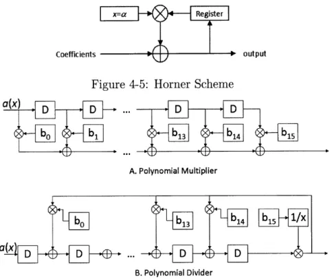
Another frequently used function in Galois Field is the polynomial evaluation. The Horner's rule is commonly used because of its hardware simplicity. For example, the Horner's representation of an order 2 polynomial can be written as ao + aix + a2x2 = (a2x + ai)x + ao. The implementation diagram of the Horner's rule in Figure 4-5

Figure 4-3: The XTime function

Coefficients

Figure 4-5: Horner Scheme

a(x) D D ... _{D D} bib 1 b14 b15 A. Polynomial Multiplier b13 F 14 b15 1/ ar D.D D B. Polynomial Divider

Figure 4-6: Multiplication and Division of Galois Field Polynomials

For a polynomial of order N, it takes N + 1 cycles for the device to perform the evaluation.

Polynomial multiplication and division are two frequently used polynomial oper-ations in Galois Field. The implementation of polynomial multiplication takes the form of an FIR filter where the coefficients of one polynomial pass through the FIR filter constructed from the coefficients of the second polynomial. The polynomial division, similarly, takes the form of IIR filter, i.e., the coefficients of the dividend polynomial pass through the IIR filter constructed from the coefficients of the divisor polynomial. Their implementation diagrams are presented in Figure 4-6.

4.3

System level considerations

The throughput of LCC decoders is set to one F2. symbol per cycle. This throughput is widely adopted for RS decoders. To maintain the throughput, in each cycle the

LCC decoder assembles s channel observations rj, 0 <

j

Stage I Stage II Stage Ill Stage IV 256 cycles 169 cycles 1 161 cycles 1 98 cycles

Stage V Stage VI 237 cycles 169 cycles

-Pbytime

Likelihood

Erasure Only Decoder, (EOD)

,0:11

Syndrome Build Error Forney Interp. Interp. RCF & Error Cact 0 (x) Calculation Poly. A S 1 Seval.

andy

i Sort by1 Build Eras. Dadorn j

y re oc. PolY - y =equyn+ia

-- ---- Ray e(x)---Evaluate v(a1). . . . . forii Ef iRC & ErrorJ Sort~~oc 0[j Codealc. SI Sequential

---- - - --- Reay , 2to l'arallel

Relayy~ y ....I . . . . . -

---Figure 4-7: VLSI implementation diagram.

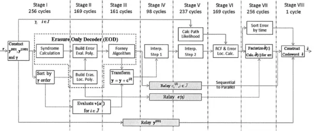
decoding procedure in our LCC implementation is divided into 8 pipeline stages, as shown in Figure 4-7. Each stage has different latencies, determined by their individual internal operations (as marked for LCC255 decoder in the figure). There is a limit on the maximal pipeline stage latency, which is determined by the (maximum) number of computation cycles required by atomic operations, such as "Syndrome Calculation". It is appropriate to set the maximum latency to 256 cycles and 32 cycles for LCC255 and LCC31 decoders respectively.

The maximum stage latency is set to ensure that the required throughput is met in each stage. As long as we stay within the latency limit, we can maximize the computation time of individual components, in exchange for their lower complexity. Thus, to trade-off between device latency and complexity, we adopt the

"complexity-driven" approach in our design.

Detailed description for each pipeline stage is provided in the following sections.

4.4

Pre-interpolation processing

As shown in Figure 4-7, Stages 1, 11 and III prepare the input data for interpolation. Coordinate transformation (described in Chapter 2) is implemented in these stages. The codeword cH, required for transformation in (2.13), is obtained using a simplified HDD decoding algorithm known as the erasure-only decoder (EOD). In the EOD, the

Figure 4-8: Data and reliability construction

N - K non-MRSP symbols (in the set T) are decoded as erasures [23]. In order to

satisfy the stage latency requirement, the EOD is spread across Stages 1, 11 and III, indicated by the dashed-line box in Figure 4-7. The operations involved in Stages I, II and III are described as follows.

4.4.1

Stage I

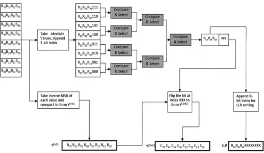
Stage I contains three main components. In the component labeled "Construct y[HD] [2HD] and 7", channel data enters (each cycle) in blocks of 8s bits; recall there are s channel observations rij per F21 symbol, and each rij is quantized to 8 bits. Symbol decisions y HDI and y42HD] are computed, as well as the reliability values -yj in

(2.10); using combinational circuits, these quantities are computed within a single cycle. Figure 4-8 presents the logic diagram of the circuit. For convenience, the di-agram considers 4-bit signal instead of 8-bit resolution in our real design. To form a Galois symbol in y[HD], we simply compact the sign bits of s corresponding input samples. The reliability values, or the log likelihoods (LLR) are obtained by finding the minimum absolute value from these s input samples. Finally, y[ 2HD] is obtained

by flipping the least reliable bit in each symbol of y[HD].

In the "Sort by -y order" block, the LRSP set I (see (2.11)) is identified as shown in Figure 4-9. A hardware array (of size jj = 16 for LCC255) is built to store partial

set set

Figure 4-9: Sort by the reliability metric

computations for I. In each cycle, the newly computed reliability 7j, is compared with those belonging to other symbols (presently) residing in the array. This is done to decide whether the newly computed symbol, should be included in the set LRSP I.

If positive, the symbol is inserted into I by order. The dash line in Figure 4-9 divides

the circuit into the main body and the control part. The registers Ej, 0 < i

<

duplicated in both parts for convenience. Based on the metrics (reliability) of the new input and the current registers, the control part produces control signals to the MUX's in the main body. A MUX in the main body has 3 inputs from the current register, the previous register and the new data. The control signal "INS" lets the new data pass the MUX. The signal "SFT" passes the value from the previous register. If none of the signals are on, the value of the current register passes the MUX so that its value is hold. The "set" signal of each register resets the reliability metric to the maximum value in initialization.

In the "Syndrome Calculation" block, we compute syndromes for EOD

[23].

1 PD D ma D

a0 01 ak-1

Figure 4-10: Compute the error locator polynomial

4.4.2

Stage II

In Stage II operations belonging to the EOD are continued. The component labeled

"Build Eras. Loc. Poly." constructs the error locator polynomial [23] using the

equation (aox + 1)(aix + 1)...(aklx + 1), where ao, ai, ...ak_1 corresponds to the

k = N - K least reliable locations in j marked as erasures. The implementation diagram is given in Figure 4-10. Note that the EOD error locator polynomial is exactly equivalent to the polynomial e(x) in (3.1); thus e(x) is first computed here, and further stored for re-use later.

The "Build Error Eval. Poly." component constructs the evaluator polynomi-als [23], which is obtained by multiplying the derivative of the error locator poly-nomial and the syndrome polypoly-nomial. The implementation device is the Galois Field polynomial multiplier as described in Figure 4-6. In Stage II the polynomial

v(x) = ] j (z - ai) in (2.14) is also evaluated over the N - K symbols in J. Its implementation is N - K parallel evaluators implemented in a similar way to the

Horner's rule. The evaluation results are passed to the next Stage III for coordinate transformation. The total number of cycles required for evaluating v(x), exceeds the latency of Stage II (see Figure 4-7). This is permissible because the evaluation results of v(x) are only required in the later part of Stage III (see Figure 4-7). In accordance with our "complexity-driven" approach, we allow the "Evaluate v(a&) for i E " component the maximum possible latency in order to minimize hardware size; note however that the total number of required cycles is still within the maximal stage latency (N + 1 cycles).

4.4.3

Stage III

In Stage III, the "Forney's algorithm" [23] computes the N - K erasure values.

After combining with the MRSP symbols in 5, we complete the clk codeword. The

N - K erasure values are also stored in a buffer for later usage in Stage VIII. The

complete c[H is further used in the component labeled " Transform

yr

+

values of v(x) have already been computed in Stage II). Finally, the transformed values

(y[HD +C) 1 -)v(ai)1 and (Y 2HD} + _v(a)1 are computed for all i

E

The operations involved in this stage are Galois Field addition, multiplication and division. The implementations of addition and multiplication are presented in Figure 4-2 and 4-4. Division is implemented in two steps. Firstly, the inverse of the divisor is obtained with a lookup table. Then the lookup output is multiplied with the dividend and the division result is obtained.

4.5

Interpolation

Stage IV and Stage V perform the critical interpolation operation of the decoder. The interpolation operation over a single point is performed by a single interpolation unit [2]. The optimization of interpolation units and the allocation of these devices are two design aspects that ensure the accomplishment of the interpolation step within the pipeline latency requirement.

4.5.1

The interpolation unit

Interpolation over a point consists of the following two steps:

PE: [Polynomial Evaluation] Evaluating the bivariate polynomial

Q(x, z) (partially

interpolated for all preceding points, see [2]), over a new interpolation point.

PU: [Polynomial Update] Based on the evaluation (PE) result and new incoming

data, the partially interpolated Q(x, z) is updated (interpolated) over the new point [2].

A. Direct Approach

~ C

icycles-SConditionL

I

B. Piggyback Approach

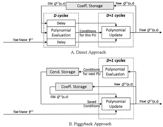
Figure 4-11: Direct and piggyback approaches for interpolation architecture design.

The PE step involves first evaluating both polynomials qO) (x) and ql) (x), be-longing to

Q

deg q,(x) are D. If both deg qo(x) and deg q,(x) are evaluated in parallel (using Horner's rule), then evaluating Q(x, z) (in the PE step) requires a total of D + 1 cy-cles. The PU step takes D +2 cycles for the update. If we adopt the direct' approach shown in Figure 4-11.A, both PE and PU steps require a total of 2D + 3 cycles.

The order of PE and PU in the direct approach is the result of PU's dependence on the conditions generated from PE since both belong to the same interpolation point, see [2]. However, it is possible to perform PE and PU concurrently if the PE step belongs to the next point. Figure 4-11.B shows our new piggyback architecture, where the total cycle count is now reduced to D + 2 (almost a two-fold savings). In this new architecture, PE is performed concurrently, as the PU step serially streams the output polynomial coefficients. Note that dedicated memory units are allocated for each interpolation units.