HAL Id: hal-01137953
https://hal.archives-ouvertes.fr/hal-01137953
Submitted on 2 Apr 2015
HAL is a multi-disciplinary open access
archive for the deposit and dissemination of
sci-entific research documents, whether they are
pub-lished or not. The documents may come from
teaching and research institutions in France or
abroad, or from public or private research centers.
L’archive ouverte pluridisciplinaire HAL, est
destinée au dépôt et à la diffusion de documents
scientifiques de niveau recherche, publiés ou non,
émanant des établissements d’enseignement et de
recherche français ou étrangers, des laboratoires
publics ou privés.
Distributed under a Creative Commons Attribution| 4.0 International License
Semi-Automatic Floating-Point Implementation of
Special Functions
Christoph Lauter, Marc Mezzarobba
To cite this version:
Christoph Lauter, Marc Mezzarobba. Semi-Automatic Floating-Point Implementation of Special
Func-tions. IEEE 22nd Symposium on Computer Arithmetic, ARITH 22, Jun 2015, Lyon, France. pp.58-65,
�10.1109/ARITH.2015.12�. �hal-01137953�
Semi-Automatic Floating-Point Implementation
of Special Functions
Christoph Lauter
∗and Marc Mezzarobba
∗†∗Sorbonne Universités, UPMC Univ Paris 06, UMR 7606, LIP6, F-75005, Paris, France †CNRS, UMR 7606, LIP6, F-75005, Paris, France
[email protected], [email protected]
Abstract—This work introduces an approach to the computer-assisted implementation of mathematical functions geared toward special functions such as those occurring in mathematical physics. The general idea is to start with an exact symbolic representation of a function and automate as much as possible of the process of implementing it.
In order to deal with a large class of special functions, our symbolic representation is an implicit one: the input is a linear differential equation with polynomial coefficients along with initial values. The output is a C program to evaluate the solution of the equation using domain splitting, argument reduction and polynomial approximations in double-precision arithmetic, in the usual style of mathematical libraries.
Our generation method combines symbolic-numeric manipu-lations of linear ODEs with interval-based tools for the floating-point implementation of “black-box” functions. We describe a prototype code generator that can automatically produce implementations on moderately large intervals. Implementations on the whole real line are possible in some cases but require manual tool setup and code integration. Due to this limitation and as some heuristics remain, we refer to our method as “semi-automatic” at this stage.
Along with other examples, we present an implementation of the Voigt profile with fixed parameters that may be of independent interest.
I. Introduction
Fixed-precision floating-point (“FP”) operations come with varying performance and accuracy guarantees. Basic oper-ations such as multiplication are typically implemented in hardware and, being correctly rounded, provide perfect ac-curacy. So-called elementary functions like exp and log are provided in software through general-purpose mathematical libraries (libms). They are well-optimized for performance and either correctly rounded, as recommended by the IEEE754 Standard [16], or provided with maximum error not exceeding one unit in the last place.
This work is concerned with special functions, i.e., “func-tions which are widely used in scientific and technical appli-cations, and of which many useful properties are known” [12]. Some, like Bessel functions or the Gaussian error function, are present in some libms. Most are provided by specialized libraries such as GSL or Root. Others are only available in computer algebra systems like Maple and Pari and have no efficient fixed-precision implementation. The NIST Digital Li-brary of Mathematical Functions[1] contains a good overview of existing implementations.
There is a huge gap in both performance and rigor be-tween these implementations and state-of-the-art elementary functions. However, implementing or reimplementing special functions manually in the classical way is tedious and requires considerable expertise. And indeed, in many cases, publicly available implementations of a given special function all derive from a single source, typically Cephes [23].
This article presents the first results of a project exploring the implementation of special functions through automatic code generation. In our view, this is the only feasible way to implement wider classes of special functions while bridging the quality gap with respect to elementary functions. Addi-tionally, code generation allows for production of specialized implementations taylored to specific applications, in terms of accuracy, supported domain or code properties.
Our focus is on special functions satisfying linear ordinary differential equations of the form
pr(x) f(r)(x)+· · ·+p1(x) f′(x)+p0(x) f (x) = 0, pi∈Q[x]. (1)
Such functions are called D-finite or holonomic. A key idea in the field of D-finite functions is that an equation such as (1) along with initial values makes up a concise exact representation of its solution that can be used in computations.
Many common special functions can be defined this way. Among the better known special functions of mathematical physics, univariate D-finite functions include in particular the error function (and related functions such as the Dawson functions or the Voigt profile), the Airy functions (as well as Scorer functions, generalized Airy functions. . . ), the Bessel and Hankel functions, the Struve functions of integer order, the hypergeometric and generalized hypergeometric functions, the spheroidal wave functions, and the Heun functions.
Under the term code generator, we understand a software tool which takes as input a description of a function f , a set of floating-point inputs X and a target accuracy ε > 0, and which generates source code (in our case, in C) that provides a function ˜f satisfying ∀ x ∈ X, ˜f(x) − f(x) f(x) ≤ ε. (2) In this work, we consider inputs in IEEE754 double precision (binary64) format taken in a relatively small interval [a, b], say of width b − a < 100, and accuracies compatible with that format, i.e., 2−53 ≤ ε ≤ 1. These restrictions can be loosened
with some manual work so that implementations on the whole set of double precision numbers become feasible.
Code generation for mathematical functions is not en-tirely a new idea. A powerful toolbox, including in particular Gappa [8] and Sollya [6], has been developed in recent years to help human developers with the most tedious steps of the implementation process. Building on these advances, several authors have considered code generation both for “flavors” of a fixed function and for “black-box” functions given as exe-cutable code [19], [9], [3], [18], [4]. Independently, Beebe [2] produced a new, very extensive mathematical library with the help of semi-automatic code generation. We base our work on the black-box approach of [19], where the starting point is ex-ecutable code able to evaluate f and its first few derivatives on intervals, up to any required precision. Providing such an evaluator is easy when f is a composition of basic elementary functions, thanks to multiple-precision interval libraries, but it is a major limitation for more general functions.
Nevertheless, if f satisfies some kind of functional equa-tion, any rigorous arbitrary-precision numerical solver could in principle play the rôle of the black box. In the case of D-finite functions, such solvers can be built in practice [25], [31]. Moreover, the behavior of D-finite functions in the neigh-borhood of their singularities is well-understood, opening the door to further extensions of the method. These observations were, in some sense, the starting point of the present work. We soon observed that the interval black-box model it is not well suited to our case, as the number of queries to the func-tion tends to be very large. This led us to favor a different interface, based on polynomial approximations, as described in Section II.
This article is organized as follows. Section II describes the general architecture of our function generation pipeline and introduces our prototype implementation. Section III focuses on the frontend part, that is, the rigorous ODE solver. Sec-tion IV discusses the backend, which is the part in charge of floating-point implementation choices. The remaining section presents experimental results and applications.
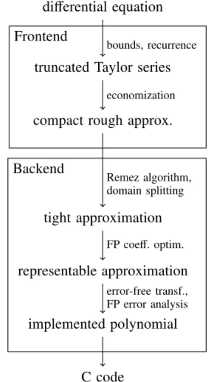
II. Overall architecture
This text describes both an approach to code gener-ation for D-finite functions and experiments performed with a prototype implementation of this approach. Our prototype, named Frankenstein, is available from https://gforge.inria.fr/git/metalibm/frankenstein.git. It is based on modified versions of two existing software packages, Met-alibm [18], written in Sollya [6], and NumGfun [21], written in Maple. The name should give a pretty accurate idea of how the combination is realized. Thus, not all design choices have the same significance: while some would survive a cleaner rewrite, others are only justified by the goal of producing a usable prototype out of two research-quality codes that had never been intended to work with each other. Here we focus on the former category, with brief mentions of more peculiar features of Frankenstein as necessary.
differential equation
truncated Taylor series
compact rough approx.
tight approximation representable approximation implemented polynomial C code bounds, recurrence economization Remez algorithm, domain splitting FP coeff. optim. error-free transf., FP error analysis Frontend Backend
Figure 1. A piecewise polynomial approximation pipeline.
Consider a sufficiently small interval I = [a, b] ⊂ R and
a solution f of (1) defined on I. Assume for simplicity that 0 ∈ I and pr(x) , 0 for x ∈ I. The function f is then analytic
on I, and the vector of initial values F(0) = ( f (0), . . . , f(r−1)(0))
characterizes f among the solutions of (1). Assume addition-ally that | f (x)| ≤ 21024(1−2−53) for x ∈ I. Then, special
floating-point values (NaN, ±∞) occur neither on input nor on output. Denoting by F the set of double-precision numbers, our goal is to produce a program computing a value ˜f(x) ∈ F satisfy-ing (2) with X = I ∩ F.
Our method takes as input (pi)ri=0 and F(0) (which together
define f ), I, ε, and various constraints on allowable imple-mentations. It either succeeds and produces a program satisfy-ing (2) by construction1, or fails if no implementation fitting
the constraints is found. Failure does not imply that no feasible solution exists.
One way to view the process leading from the definition of f by (1) to an implementation is as a rigorous piecewise polynomial approximation pipeline, as illustrated on Figure 1. Each stage receives a set of approximations of f (and possibly its first few derivatives) by polynomials on subintervals of I and produces approximations with different properties that are passed on to subsequent stages. The subintervals vary from stage to stage, and typically overlap even within a single stage. For example, the domain splitting procedure can use both a rough approximation on the whole domain to get a general picture of the behavior of f , and tight approximations on tiny intervals to compute precise values.
1This is not entirely true of Frankenstein yet. Although the overwhelming
The complete pipeline can be approximately divided into a frontend and a backend. Roughly speaking, the frontend is the part where decisions are driven by the analytic proper-ties of f . The backend is the part where they are driven by the floating-point environment and other implementation con-straints. To work with another class of mathematical functions, one would replace the frontend; to target a different evaluation environment (fixed-point arithmetic, say), one would swap out the backend. There is no formal abstraction of how the back-end can query the function, though, and both parts have full knowledge of the implementation problem.
In Frankenstein, the frontend and the backend respectively correpond to NumGfun and Metalibm. For convenience rea-sons, the process is driven by the backend, which can ask the frontend for approximations of variable quality on vari-ous subintervals. As we reuse code written for the black-box function model, the backend mostly uses these approximations to perform interval evaluations, but we expect to make more direct use of the polynomial representation in future develop-ments.
Our general implementation strategy fits the standard pattern of special function implementations and is especially close to that of Harrison [14]. Classical argument reduction algorithms based on algebraic properties of elementary functions typically do not apply. Accordingly, the only feature of f that we con-sider to reduce the implementation domain is its parity. Parity properties can be detected either by numerical comparison of f(x) and f (−x) (as Frankenstein currently does), or based on the differential equation. Periodic functions could be handled in a similar way but are very uncommon.
We then single out a small number of “interesting points”, the neighborhood of which need to be handled in a special way. Under our working hypotheses, interesting points include x =0, where the floating-point grid is denser than usual, and the points x with f (x) ≃ 0, where obtaining a relative error bound requires special care. In a more general setting, one would add at least ±∞ and the singularities of f to the list. In a small interval around each interesting point, approxima-tions of f are computed and implemented in a way that takes into account the special constraints. The remaining subinter-vals (if any) are further subdivided until approximation by small-degree polynomials becomes feasible.
Let us now consider in more detail the main ingredients of the process, starting with the frontend.
III. From a differential equation to rigorous approximations The frontend’s rôle is to provide the backend with rigorous polynomial approximations of f of the form
∀x ∈ J, | f (x) − p(x)| ≤ η (3) for various subintervals J ⊆ I. As Equation (3) suggests, in our architecture, the approximations come with absolute error bounds. Indeed, these are often easier to obtain and this choice does not hinder the use of relative error bounds in later stages. Values of J above can range from point intervals J = {x} to J = I. It is not necessary that the frontend be able to find
approximations on arbitrarily wide intervals, as the backend has the necessary logic to split J if the returned error bound is infinite (or too large). The only requirement is that sufficiently precise queries on sufficiently thin intervals eventually produce satisfying approximations.
The smallest useful value of η in our setting is slightly less than the smallest subnormal number, 2−1074. In principle, it
would be possible to replace f once and for all by a set of polynomial approximations achieving such an accuracy. The frontend of Frankenstein is more flexible and can compute arbitrarily good approximations. Precise polynomial approx-imations on wide intervals quickly become large and costly to compute. For historical reasons, our frontend provides a separate interface dedicated to points and very thin intervals that always returns “polynomial approximations” reduced to constants, which can reach absolute precisions log η−1 in the
hundred of thousands if necessary.
The computation of the approximations (3) is based on a combination of classical techniques that we now summarize. We refer the reader to [31], [21] for details.
A. Transition matrices
Recall that f is specified by the differential equation (1) and the vector of initial values F(0), or, to be precise, rigorous ar-bitrary precision approximations of F(0). Let us also extend the notation F(x) = ( f (x), . . . , f(r−1)(x)) to arbitrary x.
Polyno-mial approximations on an interval J ⊆ I will be derived from the Taylor expansion of f around the center c of J. This ex-pansion is easily computed from the differential equation and the “initial value” F(c). To deduce F(c) from F(0), we use Taylor expansions at intermediate points x0=0, x1, . . . ,xn=c
chosen in such a way that xk+1 lies within the disk of
con-vergence of the Taylor expansion of F at xk. In other words,
our frontend is essentially a rigorous ODE solver based on the so-called method of Taylor series [20].
More precisely, we proceed as follows [7], [31]. By linearity of (1), for all x, y ∈ I, there exists a matrix ∆x(y) ∈ R
r×r
depending only on (1) (not on the particular solution f ) and such that F(y) = ∆x(y) F(x). We have ∆x(z) = ∆y(z) ∆x(y) for
all x, y, z, and hence
F(c) = ∆0(c)F(0) = ∆xn−1(c) . . . ∆x1(x2) ∆0(x1) F(0). (4)
The entries of ∆x(y) are values at y of solutions of (1)
corre-sponding to unit initial values at x (or derivatives thereof). De-noting by ρ(x) the distance from x to the nearest complex root of the leading coefficient pr of (1), the Taylor expansion at x
of any solution of (1) has radius of convergence at least ρ(x). It is a classical fact that the coefficients of these expansions obey linear recurrences with polynomial coefficients, making it easy to compute as many terms as needed. As we assumed that prdoes not vanish on I, computing F(c) reduces to
form-ing the product (4), where each factor ∆x(y) can be evaluated
by summing convergent power series whose coefficients are easy to compute. Binary splitting can be used to compute the partial sums efficiently to very high precisions [7].
Our assumption that the initial values are provided at a point of I is artificial: the above argument still works with 0 < I as long as the leading coefficient pr(x) of (1) does not vanish
between 0 and I. In addition, (1) actually defines f for complex values of x, and nothing prevents the path (x0, . . . ,xn) from
going through the complex plane. If pr(s) = 0 for some s
between 0 and I, analytic continuation along a path avoiding s still defines f on I (in general in a way that depends on the path). Furthermore, when 0 < I, we can relax the assumption that pr(0) , 0: the theory extends to the case where 0 is a
so-called regular singular point of (1) [32], [21]. Both of these extensions are supported in Frankenstein, albeit with specific tool setup and subject to heuristic error estimates in some cases. The second one is useful because many classical special functions are best characterized by their behavior at regular singular points of their defining equation. A typical example is the family of Bessel functions (see Example 3 below). B. Error bounds
It is crucial that the frontend provides rigorous error bounds on the approximations it computes, as these approximations are the backend’s only access to the function f . Here, we recall a simple bound computation technique based on the theory of majorizing series [15, Chap. 2]. Frankenstein (via NumGfun) actually uses a more sophisticated variant of the same technique [22], but the present version conveys the main ideas and would probably suffice for our purposes.
Consider a power series with matrix coefficients (or, equiva-lently, a matrix of power series) Y(x) = P∞
n=0Ynxn∈R
r×r[[x]],
and let k · k denote a matrix norm. We write Y 4 w if w(x) = P∞
n=0wnxn ∈R+[[x]] is a power series that bounds Y
coefficient-wise, i.e., kYnk ≤ wn for all n ∈ N. The method
transfers such bounds on the coefficients of differential equa-tions to similar bounds on the soluequa-tions.
Our goal is to control the error committed by truncating the Taylor expansions of a solution of (1). Without loss of generality, we restrict ourselves to Taylor expansions at the origin. Rewrite (1) in matrix form, as
Y′(x) = P(x)Y(x), (5)
where P ∈ Q(x)r×r is a companion matrix with entries of
the form p(x)/pr(x), and for notational simplicity Y is also
taken to be a matrix. The matrix function P admits a conver-gent power series expansion at 0, whose coefficients Pnsatisfy
||Pn|| = O(αn) for all α > ρ(0)−1. Given such an α, it is not
too hard to compute M > 0 such that P(x) 4 q(x) := αM
(1 − αx).
Expanding both sides of (5) in power series and collecting the matching powers of x, we obtain
(n + 1)Yn= n
X
j=0
PnYn− j. (6)
The same reasoning applied to the equation w′(x) = q(x)w(x)
yields (n + 1)wn= n X j=0 qnwn− j. (7)
Now assume w0 >kY0k. Comparing (6) with (7), we see by induction that Y(x) 4 w(x). But the second equation is solvable in closed form: we have
w(x) = w0 (1 − αx)M.
This explicit expression makes it easy to bound the tails wnxn+
wn+1xn+1+ · · · , and hence also Ynxn+Yn+1xn+1+ · · · , which
yields truncation orders that guarantee a certain accuracy. C. Polynomial approximations
We are now ready to combine the results of the previous sections to obtain rigorous polynomial approximations on a given interval J. Write J = [c − δ, c + δ], and assume that δ < ρ(c). With the notation of Section III-A, we have
F(c + ξ) = ∆c(c + ξ) ∆xn−1(c) . . . ∆x1(x2) ∆0(x1) F(0) (8)
for |ξ| ≤ δ. Each factor (except F(0)) is given by power series that we can truncate so as to guarantee a prescribed accuracy. Error bounds on the individual factors are combined by re-peated use of the inequality
k ˜A ˜B − ABk ≤ k ˜Ak k ˜B − Bk + k ˜A − Ak kBk.
Once we replace each series by a truncation (and F(0) by an approximation with rational entries), the entries of (8) become polynomials in ξ with rational coefficients.
Thus, we compute the entries of ∆c(c + ξ) truncated to a
suitable order as polynomials in ξ and multiply the resulting matrix by an approximation of ∆0(c) F(0). The entries of the
result readily provide the first r derivatives of f . Higher-order derivatives, if needed, can be obtained by multiplying F(c + ξ) on the left by a row vector of rational functions (or polyno-mial approximations of rational functions) deduced from (1). In Frankenstein, most of these steps are performed exactly, us-ing multiple precision rational arithmetic. Roundoff errors in the remaining steps are taken into account in the result.
Taylor series typically do not provide good approximations on intervals. Additionally, the bounds of Section III-B can be quite pessimistic. For these reasons, polynomials computed as outlined above tend to have very high degree. However, due to the way they are constructed, the rescaled coefficients cnδn
quickly decrease to zero, and typically |cnξn| ≪ η for large n.
Before handing it to the backend, the frontend hence re-duces the degree of the computed polynomial p by economiza-tion[11, §4.6]: while the leading term of p is small compared to η, a multiple of the Chebyshev polynomial Tn (rescaled to
the interval J) chosen so that the leading terms cancel is sub-tracted from p. The error bound is updated accordingly. (The choice of Chebyshev polynomials makes it possible to take advantage of the fact that the error bound only needs to hold for x ∈ J, not for complex x with |x − c| < δ.) This procedure is very effective at producing polynomials of reasonable size that can easily be manipulated by the backend.
IV. From rigorous approximations to evaluation code It is the backend’s job to transform the high-degree, rough approximation produced by the frontend into fine-tuned ap-proximations with suitable FP properties and eventually, into source code. In absence of classical argument reduction tech-niques, implementation of the function is reduced to piece-wise polynomial approximation. The backend hence needs to compute four pieces of information, as discussed in the next subsections.
1) The implementation interval I needs to be split into subintervals Ik, together covering I, such that an
approxima-tion polynomial of small degree is possible over each Ik.
2) These small degree polynomials need to be computed, initially with real coefficients.
3) Connected with the approximation step is the problem of choosing an appropriate translation f (tk+ ·) on a new domain
Ik− tk. Indeed, the evaluation of the approximation behaves
better when Ik− tk is a small interval around 0.
4) The backend needs to transform the small-degree approx-imation polynomial on each subdomain into a polynomial with FP coefficients, suitable for evaluation in FP arithmetic, and generate code for that FP-based polynomial evaluation. A. Domain splitting
Given a target accuracy ε and a maximum degree d, the backend starts with computing a list of intervals Ik touching
each other in so-called split-points sk, i.e. such that Ik−1∩ Ik=
{sk}, covering the whole interval I =SkIk and such that for
each k there exists a polynomial pk∈ R[x] of degree no larger
than d approximating f on Ik with a relative error at most ε:
∀ k, ∀ x ∈ Ik, pk(x) − f (x) f(x) ≤ ε. (9) Such a splitting can be computed using an algorithm [18] based on bisection, interpolation of f in Chebyshev nodes and application of de la Vallée-Poussin’s theorem [5]. In Frankenstein, we leverage the existing Sollya procedure guessdegree[6] to implement this step.
B. Small degree polynomial approximation
On each subdomain Ik, the backend computes a polynomial
approximation pk∈ R[x] of degree at most d for the function f .
The pkare computed as minimax approximations with relative
error, using a modified Remez-Stiefel algorithm [5]. However, these polynomials with real coefficients2 are not immediately
suitable to IEEE754 FP evaluation. Several problems arise. When 0 < Ik, in particular when Ik contains values x ∈
Ik that are significantly larger than 1, Horner evaluation (or
any other Estrin-like evaluation) may behave badly. Roughly speaking, at each step qi+1(x) = ci+x × qi(x), the evaluation
error accumulated on qi(x) will be amplified by multiplication
with x when |x| ≫ 1, not attenuated [19]. After splitting Ik if
its radius is too large, we translate both the function f and the
2As the underlying Sollya environment is FP-based, any polynomial we can
exhibit has of course FP coefficients. However, as precision may be increased at will at this generation stage, the polynomials appear to have real coefficients.
interval Ik by tk to always be in the case when all x ∈ Ik− tk
stay small. In most cases, taking (a rounded value of) the midpoint of Ikis appropriate, while ensuring that the translated
argument ξ = x − tkcan be computed exactly in FP arithmetic
thanks to Sterbenz’ lemma [29], [19]. Special care is used when f has a zero in Ik(see Section IV-C). Further, tkmay be
optimized to take into account FP effects on the coefficients of the polynomial [19].
When Ikis small and the function f is symmetrical around
some point in Ik, the minimax approximation polynomial pk
tends to reflect the symmetry: some monomials have very small coefficients compared to others. This effect may hin-der FP Horner evaluation due to catastrophic cancellation but it can also be exploited to reduce the number of non-zero co-efficients of the polynomial [10].
C. Achieving relative error bounds for functions with zeros Clearly, the ratio (pk(x) − f (x))/ f (x) can stay bounded only
if f has no zero in the domain for x ∈ Ik or if pk has a
zero wherever f has one. Classical polynomial approximation theory either considers absolute error bounds or excludes func-tions with zeros. It can be extended to cover approximation with relative error of functions f with f (0) = 0 as follows: when f is known to have a zero of multiplicity m at x = 0, one computes a polynomial approximation qkof x−mf(x) and
takes pk(x) = xm· qk(x). The only requirement is not to use
Remez’ original minimax algorithm but an enhanced version by Stiefel [5].
Since the backend anyway uses approximation domains Ik−
tkcontaining 0, the technique above already makes it possible
to handle functions with a zero at some FP number. It suffices to take Ik small enough to contain a single zero of f and tk
equal to that zero in order to obtain f (tk+ξ) = 0 for ξ = 0. The
value of tk, can easily be computed with any numerical solver,
such as Newton’s iteration. No rigor is required in this step; if the zero is not correctly determined, relative error polynomial approximation will simply fail.
The technique no longer applies when f has a zero c < F. However, in this case, f is actually never zero on the FP num-bers it is to be evaluated at. This means that even if the ratio (pk(x) − f (x))/ f (x) is unbounded for x ∈ Ik, it stays bounded
over Ik∩ F. Provided that the procedure we use to bound the
relative error only takes into account FP numbers, approxi-mation of a function f with non-FP-representable zeros boils down to two subproblems: computing a minimax polynomial for f and translating the original function such that FP-based polynomial evaluation will exhibit bounded evaluation error.
The minimax polynomial can be computed as follows: the function g(x) = f (c + x) has an exact (FP-representable) zero at 0, and can be evaluated at any desired precision by comput-ing c with a rigorous Newton algorithm. In the Sollya frame-work, g is implemented by an expression tree containing a constant function c whose evaluation algorithm searches the original domain Ik for a zero of f whenever and at whatever
precision needed. This is enough for the Remez-Stiefel mini-max algorithm to be applicable to g.
Once c itself and a polynomial p(x) approximating g(x) over Ik− c are known, we set tk to c rounded to the nearest FP
number. The polynomial r(x) = p(tk− c + x) then approximates
f(tk+x) over Ik− tk∋ 0. At x = tk (the FP value nearest to c),
the translated argument ξ = x − tk is exactly zero, hence FP
Horner evaluation of r will return the constant coefficient of r, which is equal to (a rounded version of) f (c). For the FP x just after the zero, ξ will fit on a small number of bits due to cancellation in ξ = x − tk, hence FP Horner evaluation
will behave correctly, too. The accuracy of evaluation can be checked statically using Gappa as explained below.
Note, though, that the polynomial r passed to the code gen-eration step then contains coefficients involving the Newton-iteration based representation of c. In contrast, in the usual case (when f has no zero in the domain), the coefficients di-rectly come from the Remez-Stiefel minimax algorithm. D. FP code generation for polynomials
Finally, the backend needs to generate a code sequence, based on IEEE754 FP arithmetic, for each subdomain Ik, and
to connect these code sequences through a branching sequence determining the appropriate subdomain given an input x ∈ I. Generating the subdomain determination sequence is easy.
Generating the polynomial evaluation is harder. The back-end takes the following four sub-steps.
1) It determines the minimal precisions needed for the co-efficients of the approximation polynomial pk on each
subdo-main, following the approach described in [19].
2) It replaces the polynomial pk∈ R[ξ] with a polynomial
˜pk∈ F[ξ] with FP coefficients. This could be done by rounding
the real coefficients, however, equi-oscillation properties of the minimax polynomial and therefore accuracy might be affected too much. We therefore use a technique [5] based on lattice reduction which globally searches for a FP-valued-coefficients polynomial “close” to the original real-coefficients polynomial.
3) Starting with the target accuracy ε, the backend esti-mates suitable accuracies for the intermediate steps of a Horner evaluation of ˜pk. This choice of accuracies determines the
FP precisions—and, possibly, double-double or triple-double expansions—to be used in the different steps. The technique is described in [10], [19]. The backend then outputs C code for polynomial evaluation along with a Gappa [8] proof script. 4) Finally, the backends runs the proof script using Gappa, hence verifying the correctness of the accuracy estimates es-tablished in the previous step.
E. Evaluation-based vs. polynomial-based interfaces
In a cleanly designed special function code generator, the backend would take the rough polynomial approximations pro-duced by the frontend and proceed with refining them without ever returning back to the original function f . However, this would require the frontend to take into account the relative er-ror due to replacing f by a polynomial, which requires some understanding of FP properties of the eventual implementation when f has zeros in the domain.
For that reason and for reasons due to the reuse of exist-ing code, Frankenstein works in a slightly different way. The backend binds a Sollya function object, corresponding to f , to the evaluator dedicated to tiny intervals provided by the fron-tend. This would in principle be enough for the backend to run, since the backend—in all steps, even its polynomial approxi-mation ones—is purely based on (interval or point) evaluation. In practice, this simple interface is not enough. The number of function evaluations is too large to allow for reasonable code generation performance. In addition, an evaluation-based interface makes it hard to capture non-local properties of the function f , such as monotonicity.
We therefore enhanced Sollya to allow a function object, such as the one bound to the frontend’s representation for f , to be annotated with an alternate approximate representation along with a bound on the approximation error. The approx-imation polynomials generated by the frontend provide such an approximate representation. When it needs to evaluate the function f at some point or over some interval, Sollya first tries to use the annotation. If this first try is inconclusive, for instance if the approximation error is too large in view of the evaluation precision, it falls back to the original evaluator bound to the frontend. Interval evaluation using the annota-tion exploits global properties of the polynomial. In particular, monotonicity over the whole annotation interval is detected once and for all and later used to reduce interval evaluations on subintervals to evaluations at their endpoints.
That combination has given Frankenstein the necessary per-formance. We should mention however that making the anno-tation mechanism usable for our purposes required some fine-tuning in the Sollya architecture. In particular, as we have seen, the backend manipulates not only f itself, but also expression trees containing compositions of f with other functions, which need to be reflected on any polynomial annotation. In addition, code written in the evaluation-based model tends to perform high-precision evaluations with no real need (that is, to re-quest information on f that cannot have any influence on the correctness of the generated code). The whole benefit of the polynomial annotations can be lost if too many evaluations fall back to a slow arbitrary-precision evaluator that will try to satisfy these requests.
V. Examples and experiments A. Bounded intervals
As already mentioned, there is no complete guarantee that Frankenstein succeeds to implement a given D-finite function. The following experiments show how it performs on classical special functions. All these examples were handled automati-cally, with minimal manual setup. The reported timings were measured on a typical desktop computer.
We start with a simple example where the functions stays away from zero on the whole implementation domain.
Example 1: The complementary error function erfc(x) = 1 − 2π−1/2Rx
0 e−t
2
dt can be defined as the solution of f′′(x) + 2x f′(x) = 0, f(0) = 1, f′(0) = −2/√π.
-1.2e-19 -1e-19 -8e-20 -6e-20 -4e-20 -2e-20 0 2e-20 4e-20 6e-20 8e-20 1e-19 -2 -1.5 -1 -0.5 0 0.5 1 1.5 2
Figure 2. Relative overall error of generated implementation of erfc on [−2; 2].
We implemented erfc in the range I = [−2; 2], with a tar-get accuracy ε = 2−62, under the constraint that no generated
polynomial have more than 14 non-zero coefficients. Such a target accuracy slightly beyond double precision is typical for first phases of correctly rounded implementations [24], [19]. Though we excluded them above, our code generator is able to handle such accuracies in simple cases, automatically intro-ducing double-double expansions [28], [19] as necessary.
Figure 2 shows a plot of the relative error ˜f(x)/ f (x) − 1 of the implementation. Code generation took around 780 sec-onds. The code generator split I into 16 subdomains of varying length. In the subdomain I7=[−2/3; 2/3], the only nonzero
co-efficients of the generated polynomial are those of odd degree and that of degree 22, taking advantage [10] of an approxi-mate symmetry around 0. Accordingly, the Horner evaluation code for x ∈ I7performs evaluations in x2in all but one steps.
When executed, our implementation takes between 110 and 350 machine cycles per call, with most calls completing in 260 cycles. For comparison, a call to a typical libm exponen-tial takes around 80 cycles.
We then consider an example with several zeros, none of which is representable in floating-point.
Example 2: The Airy function Ai satisfies Ai′′(x) − x Ai(x) = 0, Ai(0) = 3−2/3Γ(2/3)−1, Ai′(0) = −3−1/3Γ(1/3)−1.
We implemented Ai on I = [−4.5; 0], asking for an accuracy ε =2−45. Frankenstein takes 280 seconds to generate an imple-mentation. It splits the domain into 10 subdomains. In two sub-domains polynomials with some zero coefficients are used; the generated code precomputes x2 accordingly. It can be checked
that all subdomains containing zeros of Ai(x) are translated by an amount equal to the double-precision number nearest to the zero, and an error plot confirms that the target accuracy is met even in the neighborhood of the zeros. Evaluation of the gener-ated function takes 60 to 90 cycles, with most calls completing in 72 cycles.
Our last example directly parallels Harrison’s implementa-tion of Bessel funcimplementa-tions for “small” arguments [14, Secimplementa-tion 3]. Example 3: The Bessel functions J0 and Y0 are defined as
solutions of Bessel’s equation
x f′′(x) + f′(x) + x f (x) = 0. (10)
We consider the function J0 on the interval I = [0.5; 42] with
a target accuracy of ε = 2−45. The immediate neighborhood
of 0 is excluded because (10) is singular at x = 0 (its lead-ing coefficient vanishes). For the same reason, initial values f(0), f′(0) do not make sense for an arbitrary solution of (10).
However, J0 can still be defined as the unique solution whose
value tends to 1 as x → 0. As mentioned in Section III-A, Frankenstein’s frontend supports such generalized initial con-ditions.
Code generation starting from this specification took about 33 minutes. The code generator splits the domain I into 18 sub-domains. The approximation polynomials in all subdomains have non-zero coefficients. For some subdomains containing zeros of J′
0(x), the implementer choses to store the coefficients
as double-double expansions even though it rounds the final result to double precision. Evaluation of the generated imple-mentation takes between 60 and 500 machine cycles, with most calls completing in 75 cycles.
B. Implementation on the whole real line: an example In some cases at least, automatically generated implemen-tations on bounded intervals can be combined to implement a special function on the whole set of double-precision floating-point numbers. We illustrate how this can be done on a simple example. The manual steps we take are really an instance of a method of some generality, but we leave it to future work to handle such cases without human intervention.
The Voigt profile V(x) (Figure 3) is a probability distribu-tion used in particular in spectrography, and whose computa-tion has been the subject of abundant literature [27], [30]. It depends on two parameters λ, σ > 0 and is defined for x ∈R
as a convolution of a Gaussian distribution and a Cauchy dis-tribution, V(x) = 1 σ√2π λ π Z +∞ −∞ exp−x2 2σ2 (x − t)2+ λ2dt.
A change of variable yields the alternative expression V(x) = 1 σ√2π λ π Z +∞ −∞ exp(u−x)2σ22 u2+ λ2 du, (11)
and it is not hard to see that (11) satisfies σ4V′′(x) + 2σ2V′(x) + (x2+ λ2+ σ2)V(x) = λ π, V(0) = 1 σ√2πexp λ2 2σ2 ! erfc λ σ√2 ! , V′(0) = 0. (12)
(To remain in our general setting, a homogeneous ODE can be derived by differentiating one more time.)
The Voigt profile with arbitrary parameters can be expressed in terms of the Faddeeva function, itself a renormalization of the complex error function. A general implementation of these functions, due to Johnson [17], is used for instance in the stan-dard library of the Julia programming language. Here we are interested in implementing the function V(x) for fixed λ and σ, with an overall relative accuracy ε = 2−45. In our experiment,
0 0.05 0.1 0.15 0.2 0.25 0.3 -10 -5 0 5 10 Figure 3. V(x) for σ = 1, λ =1 2. we take σ = 1 and λ = 1
2, but the method applies verbatim to
any moderate rational values.
We start with generating an implementation for x ∈ [0; 10]. With approximations having at most 11 nonzero coefficients, [0; 10] is split into 33 subdomains of width varying from about 0.1 around x = 5 to about 0.6 near the endpoints.
For large x, however, the computation of polynomial ap-proximations starting with the initial values at 0 as described in Section III is no longer feasible. Also, it would not make any sense to split [10; 21024] into small subintervals. An
obvi-ous remedy is to consider f (ξ) = V(1/ξ) on (0, 0.1). A change of variable in (12) shows that
σ4ξ6f′′(ξ)+2σ2ξ3(σ2ξ2−1) f′(ξ)+(λ2ξ2+σ2ξ2+1) f (ξ) = λξ
2
π . This equation has an irregular singular point at 0, beyond the scope of the polynomial approximation method we dis-cussed. Nevertheless, looking for solutions as formal power series yields a unique divergent series (compare to [13])
ξ2L(ξ) = ξ2+(2σ2− λ2) ξ4+(1σ4− 10σ2λ2+ λ4) ξ6+ · · · (13) whose coefficients again satisfy a simple linear recurrence. It is well-known that such formal solutions at infinity are asymp-totic expansions of “true” analytic solutions and provide good approximations for large x [26]. In the present case, the solu-tions of the homogeneous part of the equation decrease expo-nentially as ξ → 0, ξ > 0, so all solutions of the homogeneous equation share the same asymptotic expansion (13).
With our values of σ and λ, we estimated that the polyno-mial ˜L obtained by truncating L(ξ) to the order 90 satisfies | ˜L(1/x) − x2V(x)| < 2−65 for all x > 10. For the purposes of
this experiment, this truncation order was found numerically. Rigorous bounds could likely be derived by the method of Olver [26, Chap. 7]. NumGfun does not support evaluations near irregular singular points, but as ˜L(ξ) stays away from zero on [0, 0.1], we could directly pass it to the Frankenstein back-end. The resulting code uses two polynomials of degree 11 with floating-point coefficients.
We then manually combined the two automatically gener-ated codes into implementation that works correctly on the whole of F. The Voigt function is even, so the final code starts by dropping the sign of the argument. Based on a simple com-parison, it then calls either the code for V(x) around zero or computes ξ = 1/x (in double precision) and calls the code for V(1/x) around zero. -1.5e-14 -1e-14 -5e-15 0 5e-15 1e-14 1.5e-14 0 5 10 15 20 25
Figure 4. Relative overall error of our implementation for V(x).
Figure 4 shows a plot of the relative error of the imple-mentation of V. The plot covers all subdomains, both around zero and around infinity. It confirms that the accuracy target ε =2−45 is satisfied. Evaluations take 48 to 180 cycles, with most calls in the domain around zero completing in 60 cycles and most calls around infinity completing in 96 cycles.
VI. Outlook
Our prototype code generator is a step forward towards eas-ier, more adaptive and widespread implementation of special functions. However, it currently comes with several limita-tions.
First, though we expect it to succeed for all typical examples satisfying the assumptions laid out in Section II, code genera-tion might fail on some funcgenera-tions. Making it work for a given function may also require some deal of human intervention.
Second, our code generator handles double precision and double/triple-double expansions, but does not work for any other FP format, let alone, say, fixed-point arithmetic. It would be interesting to extend it in that direction, perhaps with the help of other existing code generation backends.
Finally, and most importantly, automatic code generation is currently limited to bounded domains. A major perspective for future research is to provide automatic support for evaluation near infinity and singularities of the function, similar to what we outlined in the case of the Voigt profile. This also means extending our framework to handle infinite families of quasi-regularly spaced zeros in the style of [14].
Acknowledgements
The authors are grateful to S. Chevillard, F. Chyzak, B. Salvy and A. Vaugon for interesting discussions on topics re-lated to this work, to V. Innocente and D. Piparo for suggesting the Voigt profile as a case study, and to the referees for their comments. This work was partly supported by the Agence na-tionale de la recherchegrant ANR-13-INSE-0007-02 MetaL-ibm.
References
[1] Digital library of mathematical functions, 2010, companion to the NIST Handbook of Mathematical Functions.
[2] N. H. F. Beebe, A new math library, International Journal of Quantum Chemistry 109 (2009), no. 13, 3008–3025.
[3] N. Brunie, Contributions to computer arithmetic and applications to embedded systems, Thèse de doctorat, ÉNS de Lyon, 2014.
[4] N. Brunie, F. de Dinechin, O. Kupriianova, and C. Lauter, Code gener-ators for mathematical functions, this volume.
[5] S. Chevillard, Évaluation efficace de fonctions numériques. Outils et exemples, Thèse de doctorat, ÉNS de Lyon, 2009.
[6] S. Chevillard, M. Joldes,, and C. Lauter, Sollya: An environment for the
development of numerical codes, ICMS 2010 (K. Fukuda et al., eds.), LNCS, vol. 6327, Springer, 2010, p. 28–31.
[7] D. V. Chudnovsky and G. V. Chudnovsky, Computer algebra in the ser-vice of mathematical physics and number theory, Computers in Math-ematics (D. V. Chudnovsky and R. D. Jenks, eds.), Dekker, 1990, p. 109–232.
[8] F. De Dinechin, C. Lauter, and G. Melquiond, Certifying the floating-point implementation of an elementary function using Gappa, IEEE Transactions on Computers 60 (2011), no. 2, 242–253.
[9] F. de Dinechin, M. Joldes, and B. Pasca, Automatic generation of polynomial-based hardware architectures for function evaluation, ASAP 2010, p. 216–222.
[10] F. de Dinechin and C. Lauter, Optimizing polynomials for floating-point implementation, Real Numbers and Computers (RNC 8), 2008, p. 7–16. [11] L. Fox and I. B. Parker, Chebyshev polynomials in numerical analysis,
Oxford University Press, 1968.
[12] A. Gil, J. Segura, and N. M. Temme, Numerical methods for special functions, SIAM, 2007.
[13] J. A. Gubner, A new series for approximating Voigt functions, Journal of Physics A: Mathematical and General 27 (1994), no. 19, L745. [14] J. Harrison, Fast and accurate Bessel function computation, ARITH 19
(J. D. Bruguera et al., eds.), IEEE, 2009, p. 104–113.
[15] E. Hille, Ordinary differential equations in the complex domain, Wiley, 1976, Dover reprint, 1997.
[16] IEEE Microprocessor Standards Committee, Floating-Point Working Group, IEEE standard for floating-point arithmetic, 2008, Second edi-tion.
[17] S. G. Johnson, Faddeeva package, 2012.
[18] O. Kupriianova and C. Lauter, Metalibm: A mathematical functions code generator, ICMS 2014 (H. Hong and C. Yap, eds.), LNCS, vol. 8592, Springer, 2014, p. 713–717.
[19] C. Lauter, Arrondi correct de fonctions mathématiques – fonctions uni-variées et biuni-variées, certification et automatisation, Thèse de doctorat, Université de Lyon – ÉNS de Lyon, 2008.
[20] J. H. Mathews, Bibliography for Taylor series method for D.E.’s, 2003. [21] M. Mezzarobba, NumGfun: a package for numerical and analytic com-putation with D-finite functions, ISSAC ’10 (S. M. Watt, ed.), ACM, 2010, p. 139–146.
[22] M. Mezzarobba and B. Salvy, Effective bounds for P-recursive sequences, Journal of Symbolic Computation 45 (2010), no. 10, 1075–1096.
[23] S. L. Moshier, Cephes mathematical function library, 1984–.
[24] J.-M. Muller et al., Handbook of floating-point arithmetic, Birkhäuser, 2010.
[25] M. Neher, K. R. Jackson, and N. S. Nedialkov, On Taylor model based integration of ODEs, SIAM Journal on Numerical Analysis 45 (2007), no. 1, 236–262.
[26] F. W. J. Olver, Asymptotics and special functions, A K Peters, 1997. [27] F. Schreier, The Voigt and complex error function: a comparison of
com-putational methods, Journal of Quantitative Spectroscopy and Radiative Transfer 48 (1992), no. 5, 743–762.
[28] J. R. Shewchuk, Adaptive precision floating-point arithmetic and fast robust geometric predicates, Discrete & Computational Geometry 18 (1997), no. 3, 305–363.
[29] P. H. Sterbenz, Floating-point computation, Prentice-Hall, 1974. [30] W. J. Thompson et al., Numerous neat algorithms for the Voigt profile
function, Computers in Physics 7 (1993), no. 6, 627–631.
[31] J. van der Hoeven, Fast evaluation of holonomic functions, Theoretical Computer Science 210 (1999), no. 1, 199–216.
[32] , Fast evaluation of holonomic functions near and in regular sin-gularities, Journal of Symbolic Computation 31 (2001), no. 6, 717–743.
![Figure 2. Relative overall error of generated implementation of erfc on [ − 2; 2].](https://thumb-eu.123doks.com/thumbv2/123doknet/14444009.517438/8.918.81.442.95.252/figure-relative-overall-error-generated-implementation-erfc.webp)

