Computation and predictive modeling to increase efficiency and performance in cell line and bioprocess development

(1)

Computation and predictive modeling to increase efficiency and performance

in cell line and bioprocess development

by

Aaron Baskerville-Bridges

B.Sc Chemical Engineering, University of Calgary, 2015

Submitted to the MIT Sloan School of Management and the Department of Chemical Engineering in Partial Fulfillment of the Requirements for the Degrees of

Master of Business Administration and

Master of Science in Chemical Engineering

In conjunction with the Leaders for Global Operations Program at the MASSACHUSETTS INSTITUTE OF TECHNOLOGY

June 2020

The author hereby grants to MIT permission to reproduce and to distribute publicly paper and electronic copies of this thesis document in whole or in part in any medium now known or

hereafter created,

Signature of Author _____________________________________________________________ MIT Sloan School of Management, Department of Chemical Engineering

May 1, 2020 Certified by ___________________________________________________________________

J. Christopher Love, Thesis Supervisor Raymond A. & Helen E. St. Laurent Professor, MIT Department of Chemical Engineering Certified by ___________________________________________________________________

Colin Fogarty, Thesis Supervisor Assistant Professor, MIT Sloan School of Management Approved by ___________________________________________________________________ Maura Herson, Assistant Dean, MBA Program MIT Sloan School of Management Approved by ___________________________________________________________________

Patrick Doyle Robert T. Haslam (1911) Professor, MIT Department of Chemical Engineering

(2)

(3)

Computation and Predictive Modeling for Cell Line Selection in

Biopharmaceutical Production

by

Aaron Baskerville-Bridges

Submitted to the MIT Sloan School of Management and the Department of Chemical Engineering on May 8 2020 in Partial Fulfillment of the Requirements for the Degrees of Master

of Business Administration and Master of Science in Chemical Engineering

Abstract

A critical early step in the development of a new biopharmaceutical is the selection of the master cell bank. Per FDA requirements, the same master cell bank must be used for all toxicity and clinical trials, as well as all production of the drug should it be commercialized. Developing a master cell bank is a time and labor-intensive process where thousands of clones are screened through a series of experiments.

The Berkeley Lights Beacon® platform can be used as a high-throughput screening tool in cell line development and has been shown to produce clonally-derived cell lines, suitable for the development of a master cell bank. In a typical use case, a Berkeley Lights chip is loaded with 1750 cells, data is collected related to cell growth and on-chip assays, and the top 50-100 are selected for further analysis. The methodology for selecting the top clones, however, is not standardized and individual users may select different top clones based on how they weigh the growth and assay data. As a relatively new tool, there is little literature outlining how to best use data collected on Berkeley Lights to select the “best” clones for further screening. In this project, we use Amgen’s database of Berkeley Lights experiments to determine which parameters are most predictive of performance in future fed-batch experiments. Data from 9 chips (N=13,900 pens; N=305 fed-batch experiments) was analyzed using linear and non-linear machine learning models to identify feature importance and improve cell selection methodology. The models generated show an improved ability to rank top clones compared to the currently methodology, a finding that is expected to improve average clone quality in cell line development.

Thesis Supervisor: J. Christopher Love

Raymond A. (1921) and Helen E. St. Laurent Professor, MIT Department of Chemical Engineering

Thesis Supervisor: Colin Fogarty

(4)

(5)

Acknowledgments

I would like to express my thanks and gratitude for everyone who helped make this thesis work possible. From practical advice to thesis-writing moral support, this was truly a collective effort. Professor J. Christopher Love and Professor Colin Fogarty provided invaluable guidance into biopharmaceutical processes, research methodology, and statistics. The content of this thesis was vastly improved by their guidance.

The Cell Line Development team at Amgen answered countless questions, gave numerous demonstrations, helped gather data, and became trusted friends and advisors. Jennitte Stevens, Kim Le, Chris Tan, Jasmine Tat, Jonathan Diep, Ryan Zastrow, Ewelina Zasadzinska, Chun Chen, and Natalia Gomez all made significant contributions to this work.

The rest of the staff at Amgen Thousand Oaks were always willing to answer obscure questions about data storage, coding best practices, calculation methodologies, and downstream implications. I learned a lot from everyone on site.

Both the Engineering and Management schools helped prepare me for this opportunity.

I found encouragement and support through the LGO program, and I am incredibly grateful to be part of the LGO 2020 cohort and the broader alumni network.

Finally, I would like to thank my friends and family for encouraging me to take the steps that put me in this position in the first place. I am humbled to be here.

(6)

(7)

List of Figures

Figure 1 - Drug Development timeline and selection of MCB ... 14

Figure 2 - Cell Line Development Process ... 15

Figure 3 - An OptoSelect Chip ... 16

Figure 4 - Decision points in the CLD process identified as candidates for ML ... 19

Figure 5 - Suitability framework applied to Optimizing Exports from Berkeley Lights... 20

Figure 6 - Example export based on selection criteria described by Le et al. ... 21

Figure 7 - Summary of user feedback for Berkeley Lights export tool ... 22

Figure 8 - Schematic of the data to be used and decision to be optimized ... 25

Figure 9 - Data preparation and model selection framework for Cell Line Development ... 25

Figure 10 - Histogram of Day 3 Cell Counts ... 29

Figure 11 – Example of outliers removed from dataset ... 30

Figure 12 - Example of data without correction factor applied ... 31

Figure 13 - Spotlight scores of zero-cell pens for each chip... 32

Figure 14 - Fitted values used for correction factor ... 33

Figure 15 - Adjusted spotlight score ... 33

Figure 16 - Typical experiment - Adjusted Spotlight Score vs. Pen ID ... 34

Figure 17 - Data from chip showing no difference between pens with and without cells ... 35

Figure 18 - Colinearity plot of X and Y datasets ... 36

Figure 19 - Spearman's Rho compared to Pearson R ... 39

Figure 20 – Schematic of Machine Learning framework ... 43

Figure 21 - Illustrative feature importance plot from XGBoost ... 44

Figure 22 - How performance is measured ... 45

Figure 23 - Spearman Rho of model compared to baseline ... 46

Figure 24 - Results from Assessment 1 for Growth ... 48

Figure 25 - Results from Assessment 1 for Specific Productivity ... 50

(9)

List of Tables

Table 1 - Framework for assessing suitability of CLD processes for machine learning ... 20

Table 2 - Number of records for each X variable ... 27

Table 3 - Number of variables for each Y variable ... 28

Table 4 - Model library ... 42

Table 5 - Illusatrative output from Lasso Regression ... 43

Table 6 - Baseline Spearman Rho values for specific productivity, growth, and titer ... 45

Table 7 – PLS Weightings for Specific Productivity Model ... 47

Table 8 - Results of specific productivity prediction ... 47

Table 9 - Results from assessment 2 for Growth ... 48

Table 10 - Principle Components for Specific Productivity Model ... 49

Table 11 - Results of specific productivity prediction ... 49

Table 12 - Results from Assessment 2 of Specific Productivity ... 50

Table 13 – Results of titer prediction ... 51

Table 14 - Results of Assessment 2 for Titer ... 52

List of Equations

Equation 1 - Calculation of Pearson's R ... 39

Equation 2 - Calculation of Spearman's Rho ... 39

(10)

(11)

0 Project motivation

In the development of biopharmaceuticals, the role of Cell Line Development (CLD) is to

identify which cell line will become the master cell bank used for all future production of a given biotherapeutic drug[1]. To accomplish this, thousands of cells are screened through a series of experiments designed to narrow down and ultimately identify the one or few cell lines with the best attributes such as growth, titer, and product quality.

To find better cell lines and shorten timelines, many biopharmaceutical companies have begun using high-throughput screening tools. A review by identifies numerous fluorescence based and robotic cell culture systems commercially available to both biotechnology companies and academic researchers [2]. One such example is Amgen, which has recently implemented Berkeley Lights’ Beacon® system as the first step in the cell line screening process. The Beacon® platform combines opto-electropositioning (OEP), microfuildics, and microscopy to create a ‘lab on a chip’ that can digitally perform cell culture tasks such as cloning, culturing, and assays. Le et al. demonstrated the Beacon® could be used to generate clonal cell lines with less resources than traditional CLD processes, and that data collected on the chip successfully predicted some cell line features [3]. To enhance the predictive power of this new technology, Amgen is looking to simultaneously standardize the data used in the decision-making process while also identifying and incorporating additional measures that provide information valuable to the selection of high performing cell lines.

Given the recent introduction of higher throughput and high content screening technologies for cell line development, little has been published about identifying predictive features in data-rich

(12)

high-throughput cell screening using commercial datasets. The goal of this thesis is to develop a machine learning framework flexible enough to improve decision-making today and in the future. There are many unique challenges presented by high-throughput screening data, and this thesis provides an overview of data assessment, data cleaning, and model validation approaches applicable to anyone using high-throughput screening tools. The framework is applied to

Amgen’s Beacon® data set, and the potential impact of a standardized decision-making approach compared to the current approach is assessed.

1 Background

1.1 Basics of Biopharmaceuticals

Traditional pharmaceuticals such as acetaminophen or ibuprofen are considered small molecule drugs; they have a molecular weight in the range of 150-200 Daltons and are produced through chemical synthesis. Biologic drugs or biopharmaceuticals, by contrast, are typically much larger and more complex, with many on the order of 30,000+ Daltons [4]. Biopharmaceuticals are produced by genetically engineering cells to produce a therapeutic protein. These genetically engineered cells are grown in bioreactors, and produce therapeutic proteins which are harvested, purified, and formulated into drugs for patients.

Biopharmaceutical companies are constantly testing and developing new types of therapeutic proteins – referred to as modalities – that interact with the body and diseases in different ways. The most common biologic modality is currently monoclonal antibodies (mAb), however new modalities such as bi-specific T-cell engagers (BiTE® molecules) and fusion proteins have seen drug approvals in recent years [5].

(13)

The biopharmaceutical industry is growing quickly as new modalities and drug targets are discovered. The global biopharmaceutical market is estimated at $270B in 2019 and forecasted to grow at a 8.7% CAGR through 2025 [6].

1.2 Amgen

Amgen is biopharmaceutical drug company headquartered in Thousand Oaks, CA. It was founded in 1980, and in 1989 received regulatory approval for Epogen, one of the earliest and top-selling biopharmaceutical drugs of all time. Today, Amgen is a multinational company with 21 approved drugs with focus areas in cardiovascular disease, oncology, bone health, neuroscience, nephrology and inflammation [7]. Amgen operates along the entire biopharmaceutical value chain, from R&D through regulatory approval, commercialization, and manufacturing.

1.3 The Importance of Master Cell Banks and Clone Screening

When bringing a new biopharmaceutical drug to market, drug developers must meet regulatory requirements to prove that their drug and processes are safe, efficacious, reliable, and of high quality. In the United States, drugs are regulated by the Food and Drug Administration (FDA). One challenge in assuring reliability and quality in biopharmaceutical drug production is the inherent heterogeneity of cells. Most biopharmaceutical companies today use random integration to incorporate the DNA that codes for the therapeutic protein into host cells; as such each cell will be slightly different [8]. In response to this, one regulatory requirement for biopharmaceuticals is that the cells used to produce biopharmaceuticals are ‘clonally derived’, meaning that all cells used to manufacture the drug are the direct descendants (via cell division) from a single parent cell (clone) [9]. With all daughter cells having the same parent clone, there is less likelihood of batch-to-batch variability or changes to the cell line over time.

(14)

A master cell bank (MCB) is a collection of daughter cells from the chosen parent clone, satisfying the ‘clonally derived’ requirement. Identifying which cell line will become the MCB is referred to as ‘clone screening’ and is on the critical path for drug development, since regulatory testing such as clinical trials must be done on the MCB. Once the MCB is chosen, it becomes the basis for all future production of the drug.

Identifying the ‘right’ MCB is also critical for manufacturing; a poor growing or producing clone can drastically increase manufacturing footprint or the number of manufacturing runs required to produce enough of the drug to meet patient demand [10].

Figure 1 - Drug Development timeline and selection of MCB

Choosing the MCB can take six or more months and cost hundreds of thousands of dollars. The choice of MCB affects the likelihood of regulatory approval, as well as the manufacturability of the drug. Caught between time and cost pressure of continued testing and the importance of the decision, biopharmaceutical companies are constantly looking for improved methods of clone screening.

1.4 Overview of the Cell Line Development Process

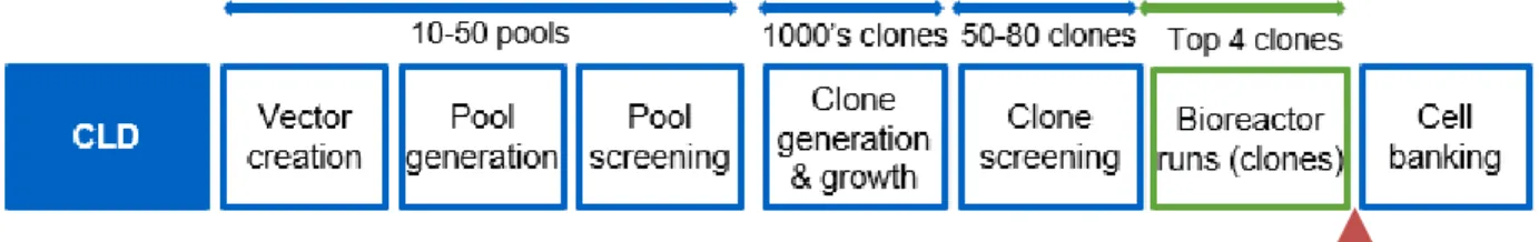
An example of the Cell Line Development (CLD) process for developing many candidate cell lines and ultimately selecting a master cell bank is described below [11]. The most commonly

(15)

used mammalian cell lines in the commercial development and manufacture of biopharmaceuticals are Chinese Hamster Ovary (CHO) cell lines [12].

Figure 2 - Cell Line Development Process

1. Vector creation: Plasmid vectors encoding for an antibody of interest are created. These vectors typically contain a selection marker such as dihydrofolate reductase (DHFR) [13]. To promote diversity and test multiple approaches, a few variants with different expression constructs may be created for a given antibody program.

2. Pool generation: The plasmids are transfected into host CHO cells through methods such as electroporation. If the cells contain a selection marker such as being deficient in

dihydrofolate reductase (DHFR), there will be a selective pressure applied: DHFR is critical to cell metabolism, and only cells which have successfully incorporated the plasmid will survive[13]. Each transfection event creates a distinct pool of many thousands of cells; these pools may have different constructs or have been transfected under different conditions. These pools are all scaled up through successive cell passages in selective growth media. Each pool is assigned a unique ID which is tracked through all future experiments. 3. Pool screening: Once pools have achieved a consistent doubling time, a fed-batch

experiment is run in 24 deep well plates. In-process samples are taken to measure cell density and viability at multiple timepoints and a final sample is taken to measure an overall titer upon completion of the experiment.

(16)

4. Clone generation and growth: The top pools identified from pool screening are advanced to clone generation. Demonstration of clonal derivation of the master cell bank is an noted in ICHQ5 guidelines and is a regulatory expectation as part of the overall control strategy [11] [15], therefore the next step in the CLD process is to isolate single cells from pools. In industry, this is done in a variety of ways, with Flourescent Activated Cell Sorting (FACS) and limiting dilution being two of the most common methods [9]. Amgen has recently validated and begun using the Berkeley Lights Beacon® platform as a method of clone generation for some cell lines [11]. The Beacon® platform can be thought of as a “lab on a chip” approach to cell line development. Each of the proprietary OptoSelectTM_{chips has} 1758 pens perfused via microfluidic channels. Single cell manipulation is performed through OptoElectro Positioning™ (OEP), which uses light to move cells into the desired area of the chip [16].

A variety of measurements can be performed on the chip, aided by the Beacon® platform’s imaging system. The entire chip can be imaged in ~8 mins, and these images are processed by an artificial intelligence algorithm to perform cell counts and ensure clonality [17].

Additionally, the imaging system can be coupled with diffusion-based florescence assays that bind to antibodies produced by the cells on the chip, allowing for measurements of cell productivity within each pen. A typical secretion assay used on the Beacon® is the Spotlight HuIg2 Assay (Berkeley Lights, Emeryville, CA). Finally, the OEP system allows for the selective export of individual pens into 96 well microtiter plates pre-filled with media.

(17)

For a typical monoclonal antibody program, 2-5 pools will be loaded on to 1-3 chips and grown on an OptoSelectTM chip for 4-5 days. This means that a typical program will have up to 5274 potential clones, not accounting for empty pens or non-clonal pens. The results of the cell count and diffusion assays are used to determine which clones have the highest potential and will be advanced for further clone screening.

5. Clone screening: While high-throughput tools like the Beacon® platform provides some initial screening capabilities, there is still uncertainty into which clone will perform best in bioreactor-like conditions. A typical export from the Beacon® will select 30-100 clones for scale-up and additional screening experiments. These screening experiments are typically conducted in flasks (30mL working volume) or small volume culture vessels such as the Sartorius Ambr [18]. Over the course of the fed-batch experiment, measurements are taken to assess cell count and viability. At the conclusion of the fed-batch experiment, samples are sent to measure the overall titer as well as further analysis such as CEX and SEC.

6. Bioreactor runs: The top clones from the fed-batch experiments are advanced to perfusion bioreactors which more closely resemble the manufacturing environment. The top 4-8 clones will be evaluated in bioreactors. Bioreactor runs make daily measurements on viability, cell density, titer, and attributes.

7. Cell banking: The top clone is selected based on performance of several parameters in the bioreactor. Multiple factors affect what is considered ‘best’ for a given program, with product quality attributes, specific productivity, titer, and growth being the most common. The top clone is expanded, and then frozen down to become the master cell bank (MCB). The MCB will last for the life of the product. Working cell banks are taken from the MCB as required for both clinical and commercial production.

(18)

1.5 Definitions of key terms used in Cell Line Development

Growth: This is measured either as a ‘cell count’ on a specific day, or as the integral of cell counts across a series of days (Integrated viable cell density, IVCD). In biopharmaceutical production, it is important to be able to scale the cell volume quickly.

Specific productivity: A measure of how much of the protein each cell produces. This is typically measured in μg/cell or or μg/cell/day and is an important parameter in sizing bioreactors.

Titer: Titer is the total amount of protein produced per unit of bioreactor volume; it is a function of the growth and specific productivity of the cell line.

Product quality attributes: Each biopharmaceutical will have different quality attributes; some examples include size (measured through size exclusion chromatography), charge (measured through cation exchange chromatography), or molecular weight. The analysis of product quality attributes typically occurs later in the CLD process than the scope of this thesis.

Clone: For the purpose of this thesis, the term ‘clone’ refers to either a single isolated cell, or a small group of cells that are all direct descendants of that cell, such as those found in a Berkeley Lights Beacon® pen.

Cell Line: For the purpose of this thesis the term ‘Cell Line’ refers to a large group of cells of clonal origin that can be grown or stored indefinitely under appropriate conditions.

Pool: A pool is a group of cells that were created from the same transfection event. Cells from a pool can be isolated to create clones. A typical chip will have 1-4 pools loaded onto it.

Program: The series of experiments and cells associated with the development of a single biopharmaceutical drug candidate.

(19)

2 Problem Definition

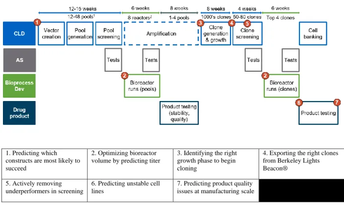
Cell Line Development consists of a series of data-informed decisions, which ultimately lead to selection of an MCB (Figure 4). At each step experiments are performed which provide better information about clones, and that data is used to decide which clone get advanced to the next step. Through conversations with CLD scientists, seven key decisions points were identified where constructs, clones, or cell lines were selected for inclusion / exclusion from future testing.

Figure 4 - Decision points in the CLD process identified as candidates for ML

1. Predicting which constructs are most likely to succeed

2. Optimizing bioreactor volume by predicting titer

3. Identifying the right growth phase to begin cloning

4. Exporting the right clones from Berkeley Lights Beacon®

5. Actively removing underperformers in screening

6. Predicting unstable cell lines

7. Predicting product quality issues at manufacturing scale

The data guiding these decisions is collected through standardized experimental approaches for thousands of clones across dozens of variables, making manual inspection challenging and opening the door to more advanced methods such as machine learning.

(20)

Table 1 - Framework for assessing suitability of CLD processes for machine learning

Component of framework Description

Current Challenges What could be improved about the process today? Is the data too complex to fully evaluate? Are too many / too few molecules being moved to the next stage? Opportunity for ML What would be the objective of ML in this situation? Is it to improve prediction

accuracy? Standardize decision-making? Reduce time spent on analysis?

Value proposition How would successful implementation affect speed to market, workload, or clone quality?

Fit with ongoing work How will this impact any ongoing work? Is this step likely to be changed soon?

Risks What are the barriers to implementation? What is the burden of proof? Who

would have to sign off on this? How could it fail?

Data Readiness What data is available for this task? How easy it is to access? Is it of high enough quality to incorporate into a ML model?

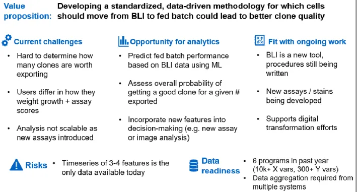
Use Case #4 - Exporting the right clones from Berkeley Lights – was selected as the most suitable project for machine learning based on the suitability framework. Figure 5 shows how this framework was applied to the Berkeley Lights Beacon® decision point.

(21)

As a high-throughput screening tool, Berkeley Lights Beacon® creates a multivariate and

extensive dataset. As a relatively new tool both to Amgen and to industry, it has not been studied in detail and there is potential for insight to be gained by more in-depth study. Finally, it is a tool well suited to machine learning since building a first principles model is challenging due to the specific nature of the chip environment and lack of genetic sequencing data on each clone [19].

2.1 Current State Analysis and Baseline

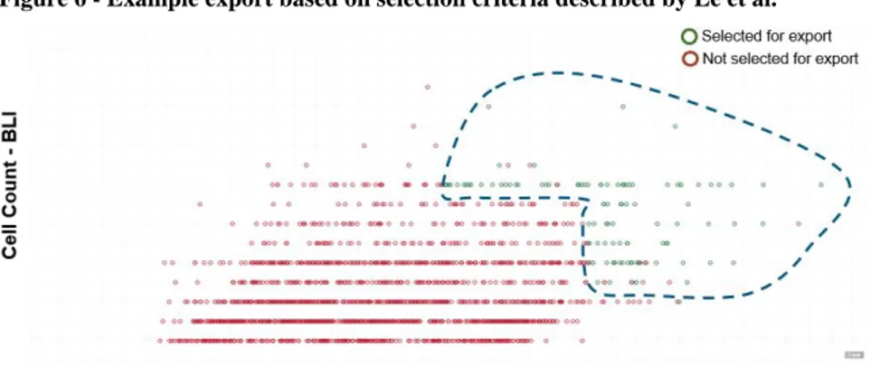
Analysis of the Berkeley Lights Beacon® data at Amgen is described in Le et al. [11]. Two features are described: 1) Secretion assays using the Spotlight HuIg2 Assay (Spotlight Assay) and 2) Cell counts using the integrated 4X microscope and camera on the Beacon® instrument.

Le et al. showed correlation between the Spotlight Assay score of a cell line and the specific productivity of that cell line in fed-batch experiments. They further described a selection

methodology whereby clones that have high Spotlight Assay scores and high growth are selected for further development in the hopes of achieving high titers. The relative weighting of these factors is left to the discretion of the scientist, and a standardized approach to scoring has not been developed.

Figure 6 - Example export based on selection criteria described by Le et al.

(22)

Specific productivity baseline: Baseline is a linear regression in Spotlight Assay Score; the higher the assay score, the higher the predicted specific productivity.

Growth: Baseline is linear regression in Cell Count; the higher the cell count, the higher the predicted growth.

Titer: Baseline is a linear regression in Spotlight Assay and Cell Count; cell lines with high scores in both will have higher predicted titers than cell lines with low scores.

In addition to comparing model performance to these performance baselines, CLD scientists also expressed a desire to know if the number of cells exported off the Berkeley Lights Beacon® could be reduced while achieving similar results. Fed-batch experiments are time-consuming and reducing the number of cells exported could free up capacity to test other cell lines.

2.2 Defining the Objective Through User Feedback

Before and during model creation, user feedback sessions with CLD scientists were conducted to understand what new analysis or insight could be created, and how any new predictive models would be used in the cell line selection process.

(23)

CLD scientists highlighted a need for a predictive tool that could rank order cells on the Beacon® and provide clarity on the relative importance of various features. Importantly, any new model should be based on all available information to that point, not just Spotlight Assay Score and Cell Count. They felt that data collected in earlier experiments, such as in the pool generation state, could provide valuable insights but was not being used in the current approach. Additionally, new assays and experiments were under development, and any model should allow easy incorporation of this data into the model and decision-making process.

Another important piece of feedback was the importance of relative rank over prediction accuracy. When using the Berkeley Lights machine, the objective is to advance the best possible clones to the next step of screening. A model that can successfully rank clones from best to worst on certain attributes is as valuable as one that can accurately predict what those values will be.

Finally, a recommendation was provided that the model should try to connect performance on the Beacon® to manufacturing or bioreactor data. This suggestion was investigated, but ultimately shown not to be feasible: of the programs run on the Beacon®, none had progressed to commercial manufacturing, and only ~30 bioreactor runs had been conducted. Instead, it was decided that the Beacon® data would be used to predict clone fed-batch performance – the next step in the process – as previous work has shown fed-batch performance to be predictive of bioreactor performance [20] and because there is much greater data availability (N=305).

(24)

3 Review of Prior Work

3.1 Berkeley Lights Beacon as a Clone Screening Tool

The foundational work to develop and test the Beacon®’s core OptoSelectTM technology was done by Mocciaro et al. [21] based on principles of optoelectric cell manipulation developed at the University of California – Berkeley [16]. Extensive work to validate the Berkeley Lights platform and define the technical procedure for commercial cell lines was conducted by the Cell Line Development team at Amgen. In particular, it was shown that common cell culture tasks could be accomplished on the Beacon® platform, that Spotlight score was correlated to specific productivity [11], and that clonality could be assured through imaging and flush procedures [3]. This published work was supplemented by in-person interviews and demonstrations at Amgen’s Thousand Oaks Cell Line Development facility.

3.2 Machine Learning Approaches Applied to Cell Line Development

A conceptual framework for applying machine learning to Cell Line Development data was developed by Yucen Xie [20]. While this worked focused on predicting titer in bioreactors further downstream than this study, many of the principles and approaches suggested were implemented in this thesis. Povey et al. used mass spectrometry data from 96 well deep plates to predict whether CHO clones would be ‘high’ or ‘low’ producers using Partial Least Squares Discriminant analysis (PLS-DA) [22]. While spectrometry data was not collected in the dataset analyzed in this thesis, PLS models were included in the analysis.

(25)

4 Solution development

The goal of this study was to determine if and how variables aside from the two used today – Cell Count and Spotlight assay score – could be used to improve the export results from the Berkeley Lights Beacon® instrument.

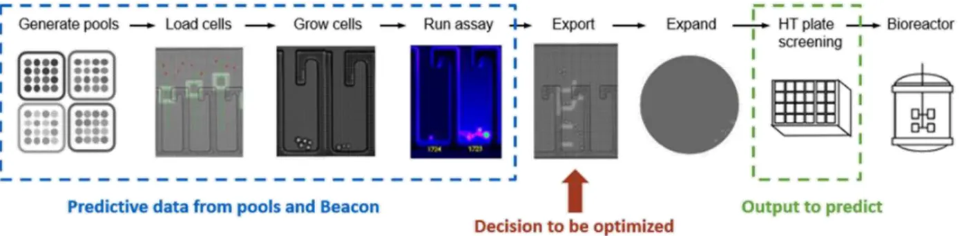
Figure 8 - Schematic of the data to be used and decision to be optimized

4.1 Data Preparation and Model Selection Framework

Many textbooks [23] and academic papers [20] outline steps to take in preparing data for machine learning algorithms. A tailored framework – provided below - was created for cell line development and applied to Amgen’s Berkeley Lights dataset.

Figure 9 - Data preparation and model selection framework for Cell Line Development

Data aggregation

• Collect data from all experiments run over the timeframe of interest

• Identify any differences in experimental procedure to investigate: different equipment, media, seeding densities, locations , scientists • Ensure consistent labeling of measured features and calculation methodology for calculated values (eg. qP, IVCD)

Data cleaning

• Decide what to do with any missing data (eg. Cells died, contamination, measurement was not taken) - impute, remove rows/columns, estimate • Investigate differences in procedure and assess whether corrections need to be made to ensure data is comparable

• Look for outliers that do not represent physical phenomena (eg. dead cells fluorescing, unachievable cell viabilities) - cap values, remove, use mean

Feature engineering

• Visualize and calculate the correlation between variables to understand which variables are colinear (eg. VCD and viability), which are correlated with the target (eg. Titer, qP, growth)

• Add calculated features to dataset for testing. Consider interaction terms, terms that account for the timeseries nature of growth (eg. IVCD)

Target & metrics

• Define the metric on which models will be evaluated. For cell line development, common metrics are RMSE if the accuracy of prediction values are important, and Spearman Rho if the rank order of predictions is more important

• Identify the metric(s) we are trying to predict. For cell line development, common targets are Titer, qP, and growth

Model selection

• Decide which models should be tested. Knowing a priori which models are best suited to each type of problem is an active area of research, but in general models commonly found in cell line development literature include PCA, Linear Regression, and tree-based models such as Random Forest • Determine validation methodology. K-fold CV may not be appropriate as it would train and test on the same cell line - which doesn't match reality

(26)

4.2 Data Aggregation

We defined the predictor variables (X dataset) as any data available before the decision to export was made. This encompasses pool fed-batch results, as well as data collected on the Beacon®. We defined predicted variables (Y dataset) as data collected during clone fed-batch experiments. The X dataset

The X dataset comprised 13,900 entries from 15,822 pens. Not all pens successfully loaded with cells, and some pens were held for reference cells. Additionally, not all features were recorded for all projects; Cell Count was done for all 13,900 pens on Day 3, but only for 5,217 pens on Day 2. The X dataset represented data from six different subcloning projects, which were run on a total of 9 chips. Each subcloning project had 3-5 pools, and overall 26 distinct pools were tested.

Some X features represent calculated values typically used in cell line development, such as the integral of viable cell density (IVCD) and specific productivity. A full summary is provided in table 2.

(27)

Table 2 - Number of records for each X variable

X dataset - Pool data X dataset - Berkeley Lights data

Predictor variable # of records Predictor variable # of records

Modality 13900 _Spotlight 13900 MTX 13900 _{CC_BLIASSAYDAY*} 13900 Pool_VCD_D00 13900 _{QP_BLI*} 13900 Pool_VCD_D03 13900 _{CC_BLID1} 8791 Pool_VCD_D06 13900 _{CC_BLID2} 5275 Pool_VCD_D08 13900 _{CC_BLID3} 13900 Pool_VCD_D10 13900 _{CC_BLID4} 3517 Pool_VIA_D00 7071 _{CC_BLID5} 1759 Pool_VIA_D03 13900 _{CC_BLID6} 1759 Pool_VIA_D06 13900 _{IVCD_BLI_D3*} 13900 Pool_VIA_D08 13900 _{DT_BLI_D3*} 8522

Pool_VIA_D10 13900 CC = cell count

Pool_Titer 13900 BLIDX = Day X after loading on BLI

Pool_IVCD* 13900 _{DT = doubling time}

Pool_qP* 13900

MTX = methotrexate * Denotes calculated value

VCD = viable cell density VIA = viability

IVCD = time integral VCD qP = specific productivity

The Y dataset

The Y dataset comprised 305 entries from 355 exported clones. Not all clones exported survived or grew to large enough viable cell densities to be recorded in fed-batch experiments. As

described in the current state analysis, clones were selected for export based on their Cell Count and Spotlight Assay score; as such our sample is biased towards clones with these properties. At this stage in the CLD process, the most important aspects of a clone to investigate were the growth, specific productivity, and titer and therefore were defined as our target variables. This is summarized in Table 3.

(28)

Table 3 - Number of variables for each Y variable

Y dataset - Fed-batch data Predicted variable # of records

IVCD_FBd10 305

Titer_FBd10 305

qP_d10 305

4.3 Data Assessment and Cleaning

Before performing any analysis or feature engineering, the data had to be assessed and cleaned. Standard steps before completing any machine learning project include handling missing data and handling outliers [23]. Additionally, since our project used data form multiple sources and experiments, we had to ensure that the data wass comparable from one experiment to the next. Handling missing data

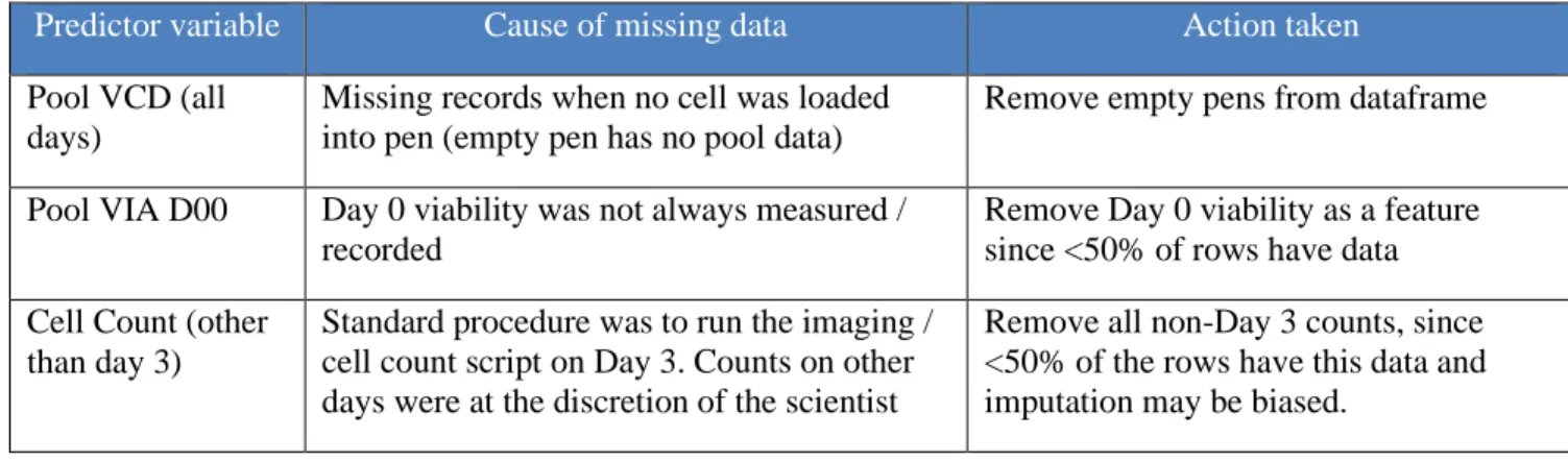
Missing data took two forms in our dataset: missing records, and zero values. From Table 2, we can see that there was significant missing data in the X dataset compared to the 15,822 available pens, reducing the X data to 13,900 pens. Results from data assessment are summarized below:

Predictor variable Cause of missing data Action taken

Pool VCD (all days)

Missing records when no cell was loaded into pen (empty pen has no pool data)

Remove empty pens from dataframe

Pool VIA D00 Day 0 viability was not always measured / recorded

Remove Day 0 viability as a feature since <50% of rows have data Cell Count (other

than day 3)

Standard procedure was to run the imaging / cell count script on Day 3. Counts on other days were at the discretion of the scientist

Remove all non-Day 3 counts, since <50% of the rows have this data and imputation may be biased.

(29)

Our Y dataset also had missing data. Data was collected only on projects that advanced to screening; therefore, we only had 355 datapoints of which 50 were terminated before completion, leaving 305 total Y datapoints.

Predicted variable Cause of missing data Action taken

Day 10 Titer, IVCD, qP

Experiment was terminated before Day 10 due to lack of growth or contamination

Since root cause was not always known, all 50 records were removed from the dataset; assigning a value of zero could bias results

Handling outliers

Outliers can be caused by variability in the process or by measurement error. For this project, we wanted to remove any outliers caused by measurement error and retain any outliers caused by outstanding performance. This classification of outliers was done through visualization / manual inspection of the datasets, as well as conversations with the scientists who collected the data.

Pool data: No outliers were found in pool data. Pool data was verified at multiple points prior to

entry into databases and the results reported have already been evaluated for outliers.

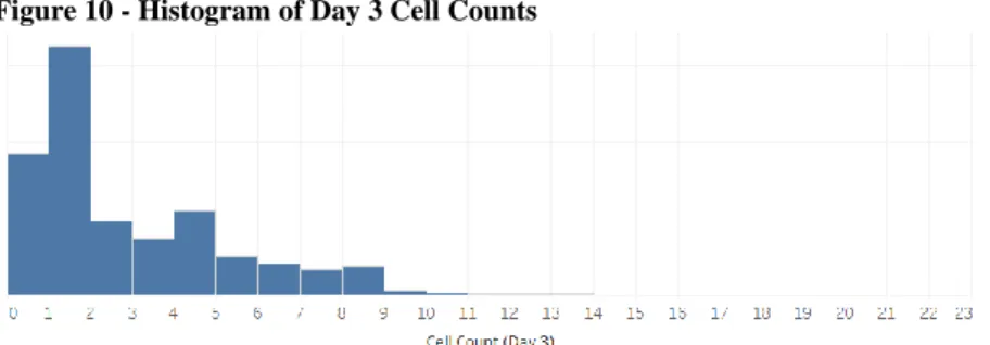
Beacon data: The main data points from the Beacon® dataset were the Day 3 Cell Count and

the Spotlight Assay Score. The Day 3 Cell count was not found to have any outliers. A histogram of the data shows the distribution of cell counts. This histogram matched expectations: some pens failed to load (0 cell counts), many pens had 1 cell loaded but it did not grow (1 cell counts) and then some cells grew:

(30)

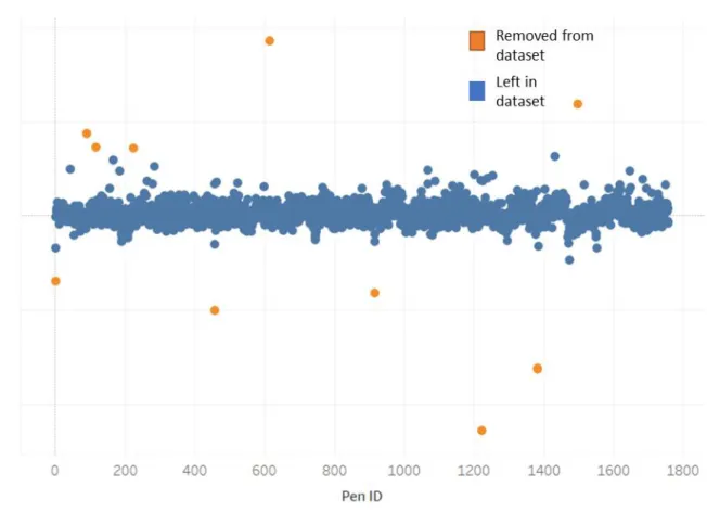
The Spotlight Assay scores, however, were found to have outliers in the form of very high and very low values. These values are artifacts from either dead cells or reference pens. None of these outlier cells were exported or have Y data; before export any high-scoring pen is manually reviewed. A heuristic was applied to all programs to remove obvious outliers: any Spotlight assay score with Z-score below -4 or above 5 was removed from the dataset. While some artifacts may remain, this will remove any obvious outliers most likely to impact any feature engineering efforts such as scaling.

Fed-batch data: No outliers were found in fed-batch data. Fed-batch data is verified at multiple

points for outliers as part of data capture.

Figure 11 – Example of outliers removed from dataset

S potl ight Assa y S core

(31)

Comparability of datapoints: Creating an adjusted Spotlight Score

By creating a combined dataset, there is an implicit assumption that each datapoint can be compared to the others. This assumption must be tested – is it fair to compare data from one pen to another? Data from one chip to another?

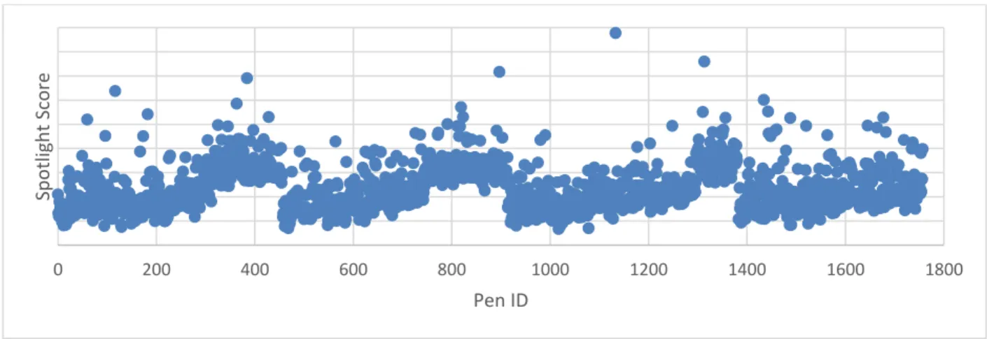
Differences in the flush rates at the inlet and the outlet of the BLI caused some pens to have artificially inflated or reduced scores. While a correction procedure involving reference images has been created by Berkeley Lights, it was discovered that not all historical data had this correction applied, and since the experiment had already been run, a reference image could not be taken post-hoc.

Figure 12 - Example of data without correction factor applied

The OptoSelect chips have four microfluidic channels, each consisting of approximately 440 pens and numbered from inlet to outlet. In Figure 10, we see the four distinct channels – an artifact of the different microfluidic flow patterns.

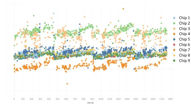
Additionally, differences in the camera or chip, artifacts on the chip, or other disruptions during calibration can cause some chips to have Spotlight scores biased higher or lower than others. In

0 200 400 600 800 1000 1200 1400 1600 1800 Sp o tligh t Score Pen ID

(32)

representing a different chip. In theory, these should all be at approximately the same Spotlight value. However, we see that there is a bias higher or lower for some chips.

Figure 13 - Spotlight scores of zero-cell pens for each chip

An algorithm was written to create a post-hoc correction. Each chip was divided into its four channels. Then, each of these 4 channels was further subdivided into 8 smaller components to capture the ‘local’ variation, rather than the biased values. In each of these sub-components, Spotlight scores with a Z score above 1.5 (representing actual signal) were removed. The remaining baseline values were used to fit a third order polynomial to each channel. The equation for the correction is: 𝑦_{𝑎𝑑𝑗𝑢𝑠𝑡𝑒𝑑} = 𝑦_𝑖 − ŷ where yi is the raw Spotlight score, ŷ is the fitted value for that pen on that chip, and 𝑦_{𝑎𝑑𝑗𝑢𝑠𝑡𝑒𝑑} is the Adjusted Spotlight Score.

(33)

Figure 14 - Fitted values used for correction factor

Figure 15 - Adjusted spotlight score

We see that the adjustment did a good job ‘fixing’ the bias created by the microfluidics and centers the baseline at zero. This allowed for comparability between chips.

0 200 400 600 800 1000 1200 1400 1600 1800 2000

Raw spotlight score Fitted values

0 200 400 600 800 1000 1200 1400 1600 1800 2000

(34)

Comparability of datapoints: Removing inconclusive experiments

Before including any experiment into the dataset, we also had to ensure that the experiment successfully measured the desired variables such as secretion (via Spotlight assay) and cell count. Results from each chip were visualized to assess whether there were any irregular results. One such result was the assessment of Spotlight assay score. Since some pens were not loaded with cells, they provided a baseline value – pens with cells should exhibit higher Spotlight scores than pens without cells.

For one chip, we did not see this pattern; instead we saw no distinction between pens with cells and pens without cells. This result was irregular and unexpected, it was likely due to instrument or materials issues, and not meaningful. The data from this chip was excluded from the final dataset.

Pens with cells Pens with 0 cells

(35)

4.4 Feature Engineering

The goal of feature engineering is to find the best representation of the predictor variables to increase the effectiveness of the model. Johnson and Kuhn [24] outline the ways this can be accomplished as:

• a transformation of a predictor,

• an interaction of two or more predictors such as a product or ratio,

• a functional relationship among predictors, or

• an equivalent re-representation of a predictor.

No fixed rules exist to determine the best feature engineering steps. Visualizing the data and using intuition into the underlying relationships is typically used to determine which feature engineering steps should be assessed for performance improvement. For example, a common ‘feature engineering’ step in biotechnology is to calculate the integral of viable cell density (IVCD) as a way to represent the time-series nature of cell growth.

Pens with cells Pens with 0 cells

(36)

Visualization of the data

As a first assessment, we plotted the linear correlation of the different variables in our X and Y datasets. Red boxes indicated positive correlation, while blue indicated negative correlation.

Figure 18 - Colinearity plot of X and Y datasets

(1) The sections highlighted in black showed a negative correlation between growth and productivity. Pools that that grew quickly tended to have lower pool specific productivity, and this carried through to fed-batch. Importantly, high growth did not make up for the lower specific productivity, resulting in lower fed-batch titers

(37)

(2) This blue box showed the high collinearity of our timeseries data for pool growth; viability and growth on the various days are highly correlated. Reducing the

dimensionality of these features may be possible through calculated values such as IVCD or using models that reduce the dimensionality of variables such as PCA or PLS.

(3) Our three main outcomes (titer, specific productivity, and growth) were all positivity correlated with pool titer and our adjusted Spotlight score – but were negatively correlated with the Cell Count on the BLI on day 3.

Titer is the product of cell growth and specific productivity; in an attempt to capture this, the product of Cell Count and Spotlight Assay was calculated.

Each subcloning project tested has different characteristics; some projects may in general be more productive or grow faster. The values for assay or growth can be scaled against cells of the same cohort to give an unbiased view of growth and assay score; ‘scaled’ values for Cell Count and Spotlight were calculated relative to other clones in the same program. Finally, squaring values is a simple feature engineering technique to capture some non-linearity in responses. From these principles, the following features were calculated and added to the X dataset.

Variable name Definition

Scaled_Au Captures the relative Adj_Au score of a clone compared to others in the same cell

line by scaling to the 25th/75th percentile scaling for that cell line only

'Au_x_CC' Adjusted Au times Cell Count – captures the interaction of these two terms

Scaled_CC Captures the relative Cell Count of a clone compared to others in the same cell

line by scaling to the 25th/75th percentile scaling for that cell line only

'Au_x_CC_Scaled' Scaled Au score times scaled Cell Count – captures the interaction of these terms

CC^2 Cell Count squared

'Au_Scaled^2' Scaled Au score squared

CC_Scaled^2 Scaled cell count squared

Pool_Titer^2 Pool Titer Squared

(38)

One-hot encoding of modality

Modality is a categorical variable. For most models tested, all data must be numerical. The most common method of transforming categorical variables to numerical values is called ‘one-hot encoding’ [25], which transforms a categorical variable with n possible values into n-1 features, as shown below: Modality mAb BiTE® XmAb® Bi-Specific

4.5 Model selection and assessment

As outlined in Section 2.2, scientists in CLD identified the most important metric for evaluating models as relative rank over prediction accuracy. The scientists were most concerned about advancing the best clones to the next experiments, rather than knowing exactly what value of growth, specific productivity, or titer they will have. Considering this, two main metrics were considered when evaluating models:

1. Spearman’s Rho – a non-parametric measure of rank correlation that assesses how well our model ranks our clones [26]. This is used extensively in cell line development and biological data assessment[27].

2. Root Mean Squared Error (RMSE) – a standard metric of model prediction accuracy

Modality-mAb Modality-BiTE® Modality-XmAb®

1 0 0

0 1 0

0 0 1

(39)

Spearman’s Rho

Spearman’s Rho (ρ) can be better suited as a model selection metric in Cell Line Development than RMSE or Pearson R due its treatment of outliers. CLD is actively looking for outlier cells; stresses are put on cells to either make them express highly, or to force many cells to die to selective pressure. Outliers create severe penalties in RMSE and Pearson R scores. Spearman Rho is calculated similarly to Pearson R, however rank orders rather than actual values are used.

This reduces the impact of outliers by effectively making all values the same distance apart. This is demonstrated in Figure 19 [28], which shows a monotonically increasing function of predicted value vs. actual value. The R2 of this is 0.88, but Spearman considers the rank order and thus ρ=1. For a CLD scientist, this is a perfect model; it accurately ranks cells from best to worst, and the decision for which clones to advance can be made.

The similarity between Pearson R and Spearman Rho can also be gleaned from their formulas; where Pearson R uses ‘x’, Spearman uses R(x) denoting the rank value.

Figure 19 - Spearman's Rho compared to Pearson R

Pr

edict

ed v

al

ue

Actual Value

(40)

As outlined in Section 1.4, the final step in the clone screening process is running the top four clones in bioreactors. A function of improved ρ should be the ability for CLD scientists to export less clones from the Beacon® while still having the confidence that they will capture the four best-performing ones. Currently the standard is to export 30-100 clones per program, but scaling and screening all these clones is time consuming. Can an algorithm pick out the top four from a smaller subset?Given the biased nature of our dataset – we can only use data from clones that were exported in the past – it is challenging to determine exactly how many clones should be exported. We developed two assessments which provide insight into the predictive power of the models selected.

Assessment 1: If we reduced the number of clones exported by 50%, which ones would the

model select for export? Would it still capture the top four clones?

Assessment 2: How many clones would need to be exported for the model to capture the top

four clones?

These assessments are limited to ranking clones which were exported using the current clone selection methodology. Our model may have suggested a different set of clones be exported, potentially resulting in better overall clones. In the future, additional assessments may be done where exports using both the current methodology and any improved model are run head-to-head and the results compared directly.

(41)

Cross validation

When training and comparing machine learning models, k-fold cross validation is commonly used to measure model performance and select the optimal hyperparameters [29]. K-fold cross validation uses a subset of the data as a ‘training set’ and tests the model on the held-out portion, and then repeats this process for k subsets of the data. This is a robust method to ensure model selection is not unduly biased by the test set selected.

In order to minimize bias in the results, the k-fold strategy should mirror the real-world considerations. Each time CLD runs experiments, it is doing so with a cell line that has never been experimented on before, and it may react slightly differently than any cell line run before it. Our goal was to model performance despite this lack of prior knowledge; therefore, our model did not train and test on samples from the same cell line. A traditional k-fold strategy randomly samples data from a dataframe; this would result with data from a given Cell Line in both the training set and the test set. Instead of a traditional k-fold validation, a custom block validation strategy was implemented. Rather than folds consisting of a random sample of the dataset, each cell line constituted one fold. This is point is illustrated below:

(42)

4.6 Predictive Models Assessed

Based on the dataset and user feedback, any models used had to meet two main considerations:

1. They had to be models that could provide a quantitative output

2. They had to be interpretable, either by providing coefficients weights for regression models or feature importance weights for tree-based models

Based on these criteria the following models were included in our model library:

Table 4 - Model library

Regression models Tree-based models

Linear regression Random Forest

Ridge regression XGBoost

Lasso

PCA w/ linear regression PLS

4.7 Machine Learning Framework

The machine learning framework and all models were implemented in a Python program using scikit-learn and pandas libraries [30] [31]. To run the program, the user selected which cell lines should be included in the dataset, which features of the X dataset should be incorporated into the model, and which Y value to predict. The program then performed all data-cleaning steps

outlined in Section 4.3, including removing zero values and outliers, and created the k-fold training-test splits outlined in Section 4.5. This cleaned train-test data was then run through each model in our model library (Table 4) over a range of hyperparameters. For each of the 6 k-fold splits, Spearman’s Rho and the RMSE were stored, and an average of the six folds was

calculated to compare model performance as defined in Equation 3.

(43)

Figure 20 – Schematic of Machine Learning framework

4.8 Feature reduction methodology

The complete dataset had 27 features with 305 measurements. This is a lot of features compared to measurements, and intuitively we expected a model with all features to overfit. To reduce overfitting, we started with a full model and then features were iteratively removed using the results from two of the models in our model library: Lasso regression and XGBoost.

Lasso is a sparsity-inducing model that shrinks parameters that are not predictive, making them candidates for removal from the dataset. In the illustrative example in Table 7, Pool Titer is more important than Spotlight which is more important than Cell Count. The program would be re-run without Cell Count and the performance compared to that of the full model.

Table 5 - Illusatrative output from Lasso Regression

Model Train set Pool_Titer Spotlight Cell Count …

Lasso Reg Cell lines 1,2,3,4,5 0.58 0.06 0 …

Lasso Reg Cell lines 1,2,3,5,6 0.72 0 0 …

(44)

XGBoost is a tree-based model. A feature importance plot shows how often each variable was split on in training the tree, which is a measure of its predictive power. A similar process to Lassso was applied; if a variable had a low importance – for example Pool_Titer^2 in the illustrative example below – it was removed and the model was re-run on the reduced dataset.

5 Results

5.1 Defining model performance

Ideally, we would have measured the performance of the model on its ability to rank order the cells in each of the Lights OptoSelectTM chip’s 1758 pens. How well did our model separate the good cells from the bad cells? Unfortunately, it is impractical to export, scale, and analyze 1758 separate samples in fed-batch experiments: each fed-batch experiment requires manual cell culture work such as changing media, taking viability samples, and analyzing titer. Instead, 30-80 pens from each chip were exported, scaled, and analyzed. As outlined in Section 2.1, these exported pens showed high Spotlight Assay scores and high growth on the chip. We therefore defined ‘performance’ as the ability of our model to rank order exported cells, which we had data

(45)

for. Because bad cells had theoretically been removed from our dataset, our measure of performance is a model’s ability to separate good cells from great cells. This is an inherently harder problem. Reported values are not an indication of the overall screening ability of Amgen’s CLD process; rather, they are an indication of model performance above and beyond the current baseline procedure.

Figure 22 - How performance is measured

5.2 Baseline Performance

As outlined in Sections 2.1 and 5.1, current decision-making procedure was used as the performance baseline against which machine learning models were evaluated. The predictive power of the current procedure in rank ordering exported clones - measured by Spearman’s Rho – was calculated for specific productivity, growth, and titer.

Table 6 - Baseline Spearman Rho values for specific productivity, growth, and titer

Variable Baseline Rho value

Specific productivity Linear regression in Spotlight Assay Score 0.468

Growth (IVCD) Linear regression in Cell Count 0.001

Titer Linear regression in Spotlight Assay Score and Cell Count 0.245 Our dataset was larger than the one evaluated in Le et al. [11], but comes to the same conclusion that Spotlight Assay Score is a strong predictor of specific productivity. Cell Count, however, was not found to be good at differentiating the growth of clones that were exported.

(46)

5.3 Model Performance

The goal of developing a program in Python was to identify models that could improve upon the baseline performance in predicting specific productivity, titer, and growth. Using the procedure outlined in this thesis, our program was run to test multiple models on our dataset and cross-validate them across a range of hyperparameters. The ‘best’ model was selected as the one with the lowest average Spearman’s rho across all cell lines for a given hyperparameter.

This procedure was able to produce improved results for all three of our target variables. The largest gain was seen in predicting growth, which went from ρ=0 (no predictive power) to

ρ=0.283 with our model. The model for specific productivity only gave small improvement, from ρ=0.468 to ρ=0.492, meaning that Spotlight Assay alone can account for most of the differences in specific productivity rank order. Finally, we saw a moderate increase in performance for Titer, with the rank correlation increasing from ρ=0.245 to ρ=0.342.

Figure 23 - Spearman Rho of model compared to baseline

0 0.1 0.2 0.3 0.4 0.5 0.6

Cell Growth Specific productivity Titer

Sp ear m an Rh o v alu e

(47)

5.4 Model Performance in Predicting Growth

The best model for Growth was found to be a PLS with one principle component. The model used nine variables and the weighting vector placed importance on Pool data, rather than data collected on the Berkeley Lights instrument. Pool Titer, Pool IVCD, and Pool Viable Cell Densities on Days 6 and 8 had the highest weightings, while Cell Count had a low weighting.

Table 7 – PLS Weightings for Growth model

Cell Count Pool_VIA_D06 Pool_VIA_D08 Pool_VIA_D10 Pool_IVCD Pool_VCD_D06 Pool_VCD_D08 Pool_VCD_D10 Pool_Titer

-0.08 0.18 0.16 0.18 0.27 0.24 0.21 0.02 0.45

Table 8 - Results of growth prediction

Model Best hyperparameter Average rho Average RMSE

Linear regression N/A .001 42.4

Ridge regression Lambda=8 .206 51.5

Lasso regression Lambda=0.19 .219 51.2

PCA Score = 2 .220 54.5

PLS Score = 1 .283 49.1

Random Forest Min leaf size = 2 .066 56.9

XGBoost Learn rate = 0.2 .098 58.9

The model results for growth show that the best indicator of growth in fed-batch is the pool the clone came from, rather than its growth on the Berkeley Lights chip. Even this has limits, however, as demonstrated by Cell Lines 3 and 5, where some of the top-growing clones were not predicted to be in the best 50%. This information is still valuable, however, when compared to the baseline of no predictive power from Cell Count alone. To ensure the top 4 growing clones were exported, a minimum of 37 clones would have to be exported based on the results from Cell Line 4.

(48)

Figure 24 - Results from Assessment 1 for Growth

Table 9 - Results from assessment 2 for Growth

# of clones exports required to capture top four

Cell Line 1 Cell Line 2 Cell Line 3 Cell Line 4 Cell Line 5 Cell Line 6

9 26 31 37 18 17

Cell Line 1 Cell Line 2

(49)

5.5 Model Performance in Predicting Specific Productivity

The best model for Specific Productivity was found to be PCA with two principle components. The model used eight variables; the first component is weighted towards the values of Pool Titer, Spotlight Assay Score, and Specific Productivity on the Beacon®, while the second component is weighted towards scaled values of these metrics, that normalize for the different characteristics of each cell line.

Table 10 - Principle Components for Specific Productivity model

Component Pool_Titer Adj_Au Pool_qP Pool_VCD_D06 QP_BLI_adj Scaled_Au Au_x_CC_Scaled Au_Scaled^2

1 0.42 0.47 0.09 -0.23 0.43 0.41 0.06 0.40

2 -0.27 -0.13 -0.24 0.20 -0.17 0.39 0.65 0.34

Table 11 - Results of specific productivity prediction

Linear regression N/A .467 17.6

Ridge regression Lambda=9 .319 11.75

Lasso regression Lambda=0.19 .449 13.67

PCA Score = 2 .492 12.80

PLS Score = 2 .459 11.69

Random Forest Min leaf size = 3 .328 15.15

XGBoost Learn rate = 0.35 .226 15.05

The model predictions of specific productivity were quite promising; even halving the number of exports conducted, only one of the 24 “top four clones” was lost across all cell lines. Even more interesting is the implications for future exports; high specific productivity can be selected for, and downstream experiments could be done to identify cells that also grew well. The maximum number of clones required to capture the top four was 31, and cell lines 5 and 6 each identified all four top producing clones within the top 8 predicted.

(50)

Figure 25 - Results from Assessment 1 for Specific Productivity

Table 12 - Results from Assessment 2 of Specific Productivity

12 13 21 31 8 7

Cell Line 1 _{Cell Line 2}

(51)

5.6 Model Performance in Predicting Titer

The best model for Titer was found to be a Ridge Regression with Lambda = 1.3, although a simple linear regression performed nearly as well. The model to predict titer was found to overfit for many combinations of variables, and in the end the top model was built using only Pool Titer and Spotlight Assay Score as inputs.

Table 13 - Ridge Regression coefficients for Titer model

Spotlight Pool Titer Intercept

0.116293 0.593201 0.830836

Table 14 – Results of titer prediction

Baseline – linear

regression on

Spotlight, Cell Count

N/A .245 .668

Linear regression N/A .340 .619

Ridge regression Lambda=1.3 .341 .616

Lasso regression Lambda=0.001 .340 .621

PCA Score = 2 .340 .619

PLS Score = 2 .340 .619

Random Forest Min leaf size = 4 .211 .674

XGBoost Learn rate = 0.5 .016 .736

The results from Assessment 1 show that a 50% reduction in exports using the model is likely too aggressive. Cell Lines 3,4 and 5 all had clones in the top 4 removed by the model, which is not favorable. To ensure all of the top 4 clones were selected, at least 38 clones would have to be exported from Cell Line 4 with the current model.

(52)

Figure 26 - Results from Assessment 1 for Titer

Table 15 - Results of Assessment 2 for Titer

12 15 26 38 21 35

(53)

6 Conclusions and Recommendations

Our goal with this project was to develop a machine learning framework that could improve which clones are exported from the Berkeley Lights Beacon®. The models developed showed improved ability to rank clones for export from Beacon® and are also flexible enough to incorporate new cell lines and new assays into the dataset as they are tested and developed. When compared to current state methods, our machine learning based model demonstrated improved performance compared to the baseline performance of current methods. Our model improved the Spearman’s Rho rank correlation value from no predictive power to ρ=0.248 for Growth, ρ=0.467 to ρ=0.492 for Specific Productivity, and ρ=0.245 to ρ=0.342 for Titer. Our cross-validation strategy held out entire cells lines as test sets, meaning that the results reflect as best as possible the ability of our model to rank order a new cell line being tested. Finally, our model uncovered relationships that can further improve the understanding of CLD processes, including the strong correlation between pool growth features and fed-batch growth, as well as limited predictive power of the Day 3 Berkeley Lights Cell Count.

There are many possible explanations for why Cell Count on the Beacon® does not correlate with fed-batch growth. Firstly, cells are grown over short periods of time – typically three days – at low cell densities on the Beacon®. Cell counts are done using the built-in microscope and an automated cell counting algorithm provided by Berkeley Lights. The chip is a static environment and the media used is specific to the Beacon® machine. In contrast, fed-batch experiments are run over 10 days in a sparged, stirred tank bioreactor at medium to high cell densities. Cells may behave differently in these two growing environments, and the cell count algorithm may not provide 100% accuracy. Additionally, the short growing time means that there is less

(54)

challenges suggest that future development could target other indicators of cell growth; for example genetic or intracellular markers of growth potential.

6.1 Future considerations to improve model performance

While our model shows better performance than the current methodology, there are opportunities to further improve the results.

Increasing the number of observations in our dataset

Our current dataset contains 305 observations of our target variables Growth, Specific Productivity, and Titer. Machine Learning algorithms perform better with more data, and in particular non-linear methods such as XGBoost can dramatically overfit small datasets [32]. One example that is expected to improve model performance is collecting samples from the same modality type. Interviews with CLD scientists indicate that in fed-batch, mAbs behave like other mAbs, BiTE® molecules like other BiTE® moleculess, etc. Our model is limited in its capacity to capture these relationships since so few experiments have been run on the Beacon® machine; our dataset contains information from six cell lines from four different modalities. With so little to compare with, we could not create modality-specific models even if they were justified. As more experiments are performed on the Berkeley Lights Beacon®, more specific and complex analysis will be possible without overfitting.

In order to efficiently increase the size of the data set, automating the data aggregation process should be considered. Currently data from three separate experiments – pool data, Beacon®, and fed-batch data – must be manually merged, which is a time-consuming process. Making this step