HAL Id: hal-01764048
https://hal.archives-ouvertes.fr/hal-01764048
Submitted on 11 Apr 2018
HAL is a multi-disciplinary open access
archive for the deposit and dissemination of
sci-entific research documents, whether they are
pub-lished or not. The documents may come from
teaching and research institutions in France or
abroad, or from public or private research centers.
L’archive ouverte pluridisciplinaire HAL, est
destinée au dépôt et à la diffusion de documents
scientifiques de niveau recherche, publiés ou non,
émanant des établissements d’enseignement et de
recherche français ou étrangers, des laboratoires
publics ou privés.
Online Via-Points Trajectory Generation for Reactive
Manipulations*
Ran Zhao, Daniel Sidobre, Wuwei He
To cite this version:
Ran Zhao, Daniel Sidobre, Wuwei He. Online Via-Points Trajectory Generation for Reactive
Manip-ulations*. 2014 IEEE/ASME International Conference on Advanced Intelligent Mechatronics (AIM),
Jul 2014, Besançon, France. �10.1109/AIM.2014.6878252�. �hal-01764048�
Online Via-Points Trajectory Generation for Reactive Manipulations*
Ran Zhao
1,2, Daniel Sidobre
1,2and Wuwei He
1,3Abstract— In various circumstances, such as human-robot interactions and industrial processes, planning at trajectory level is very useful to produce better movement. In this paper we present a near time optimal approach to plan a trajectory joining via points in real time for robot manipulators. To limit the speed variation, the path is smoothed around via-points in a limited area. The concept of online trajectory generation enables systems to react instantaneously at control level to unforeseen events. Simulation and real-world experimental results carried out on a KUKA Light-Weight Robot arm are presented.
I. INTRODUCTION
Defining robot motion by trajectories has many advantages to describe feasible motions or human acceptable motions. While a path defined by a polygonal lines doesn’t precise if the mobile must stop at via-points or smooth the corner, a trajectory describes precisely the motion. It is also well known that humans minimize the jerk of their movements [1] or that the bounding of the jerk and acceleration are necessary to limit the vibrations and the wear of mechanical parts during machining [2], [3]. In both case trajectories can describe the corresponding motion. Also, it is reasonable to replace paths by trajectories as the interface between planners and controllers, and to add a trajectory planner as an intermediate level in the software architecture.
To react to environment changes, the trajectory planning must be done in real time. Meanwhile, the robot needs to guarantee the human safety and the absence of collision. So the model for trajectory must allow fast computation and easy communication between the different components, including path planner, trajectory generator, collision checker and controller. To avoid the replan of an entire trajectory, the model must allow deforming locally a path or a trajectory. The controller must also accept to switch from an initial trajectory to follow to a new one.
In this paper we use third degree polynomial functions to describe trajectories and we propose an efficient method to generate trajectories. In the first stage, we suppose that a mo-tion planner produces a polygonal line. From this polygonal line, we build a smoothed and feasible trajectory bounded in jerk, acceleration and velocity. This corresponds to the
*This work has been supported by the European Community’s Seventh Framework Program FP7/2007-2013 “SAPHARI” under grant agreement no. 287513 and by the French National Research Agency project ANR-10-CORD-0025 “ICARO”.
1,2Ran Zhao and Daniel Sidobre are with CNRS, LAAS, 7 avenue du
colonel Roche, F-31400 Toulouse, France; and Univ de Toulouse, UPS, LAAS, F-31400 Toulouse, France.1,3Wuwei He is with CNRS, LAAS, 7 avenue du colonel Roche, F-31400 Toulouse, France; and Univ de Toulouse, LAAS, F-31400 Toulouse, France. [email protected] and [email protected] and [email protected]
type V trajectories in the classification proposed by Kroger [4]. As this operation modifies the initial free path, the new smoothed path must be checked for collision. Locally near a via-point, the path defines a subspace of dimension two and the trajectory proposed remains inside this subspace where the maximum error distance can be verified.
This paper focuses on the via-points trajectory planning for a service manipulator robot. We present related work in Section II. Soft Motion trajectory and the concept of online trajectory generation are detailed in Section III. Section IV describes a simple approach to build a smooth via-points trajectory. We explain how to manage the error in Section V. Simulation and experimental results are presented in Section VI using a 7-DOF arm.
II. RELATED WORK
Recent years have seen an increase in research in trajectory planning, especially related to the domains of Human-Robot Interactions (HRI) and high speed machining. Trajectory planning is commonly decomposed in two phases [5], firstly the selection of a path and then the generation of the trajectory, i.e. the building of a time evolution function along the path. A partial review for robotic is presented in Gaspareto et al. [6].
Probabilistic path planning methods [7] have had great success for robot motion, but they are not directly adapted to the changing robot environment of human-robot interaction. A lot of extensions like in [8]–[10] were proposed to improve reactivity. It should be noted that all these methods provide a polygonal path as output, which is impossible to follow at constant speed.
Broqu`ere et al. [11] gives a solution to compute a time optimum trajectory bounded in jerk, acceleration and velocity for an axis joining any pairs of states defined by a position, a velocity and an acceleration. For a point to point movement in an N-dimensional space, the time optimum straight-line motion is obtained by projecting the constraints on the line [12].
The trajectory planning problem can be solved in joint space or in the operational space, but kinematic models make the combined problems difficult. A method taking kinematic and process constraints into account for five-axis machining is presented in [13]. For more complex kinematics like 7-axis arm, the problem is still largely open to research.
In this paper we propose a solution to generate a trajectory from a polygonal path. The objective of the method is to build a time optimum trajectory while controlling the distance between the path and the trajectory.
III. ONLINETRAJECTORYGENERATION(OTG) A. Soft Motion Trajectory
Trajectories are time functions defined in geometrical spaces, essentially Cartesian space and joint space. The rotations can be described using different coordinates system: quaternion, vector and angle etc. The books from Biagiotti [5] on one hand and the one from Kroger [4] on the other hand summarize background trajectory material.
We choose a particular series of 3rd degree polynomial trajectories and name them as Soft Motion trajectories. A trajectory T is then a function of time defined as:
T : [tI, tF] −→ Rn (1) t 7−→ T (t) (2) Where T (t) = Q(t) = (1Q(t),2Q(t), · · · ,nQ(t)) T for joint motions or T (t) = X(t) = (1X(t),2X(t), . . . ,nX(t))T in
Cartesian space from the time interval [tI, tF] to Rn. n is the
dimension of the motion space. Without loss of generality, we suppose that all jQ(t) or jX(t), 0 ≤ j < n share the
same time intervals and that tI = 0. The continuity class of
the trajectory is C2.
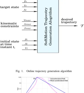
A first OTG algorithm is able to calculate a trajectory at any time instant, which makes the system transfer from the current state to a target state. A state of motion at an instant ti is denoted as
Mi= (Pi, Vi, Ai) (3)
where Pi(Pi = Q or P i = X) represents the position,
Ai the acceleration and Vithe velocity at in instant ti. Fig.1
illustrates the input and output values of OTG algorithm. We propose several trajectory generators which are capable of generating Soft Motion trajectories in one time cycle. The trajectory calculated is a type V trajectory in the classification proposed by Kr¨oger, which satisfies:
Vi ∈ Rn |jVi| ≤ Vmax
Ai ∈ Rn |jAi| ≤ Amax (4)
Ji ∈ Rn |jJi| ≤ Jmax
Pi ∈ Rn
Jmax, Amax, Vmax are the kinematic constraints and Ji is
the jerk at time ti. Therefore, at a discrete instant, the OTG
algorithm can transfer motion states while not exceeding the given motion constraints.
B. Trajectory Generators
1) Phase Synchronized Trajectory Generation: Different solutions where proposed to generate monoaxial trajectories, but for the multiaxial case, generating trajectories with the same duration is not enough and a continuous phase synchronization is necessary to define the shape of the path. For example, to generate a straight line the ratio between the velocities of each axes must be constant.
Phase synchronization is the synchronization in position, velocity, acceleration and jerk spaces. It means that, given any instant of time, all variables must complete the same
Fig. 1. Online trajectory generation algorithm
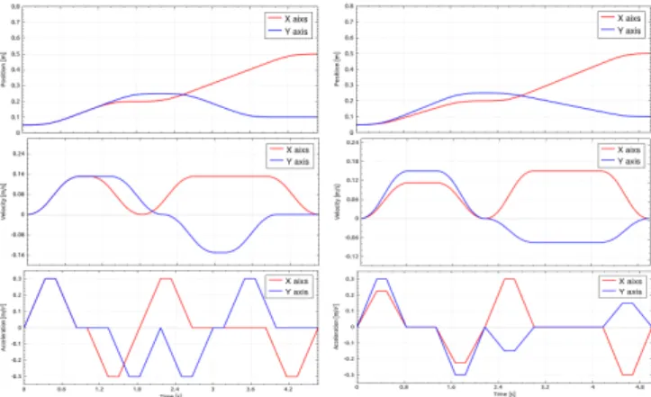
Fig. 2. Via-points motion: phase-synchronized and without synchronization
percentage of their trajectories. In a n dimensional space, Frisoli et al. [14] defines the phase synchronization as:
iX(t) −iX(tI) jX(t) −jX(tI)
= λ ∀i, j ∈ [0, n − 1], t ∈ [tI, tF] (5)
Where λ is a constant. Fig.2 illustrates the path of a simple via-points motion in 2D space. P1, P2, P3 are way points
with zero velocities and accelerations. The difference be-tween the phase-synchronized and unsynchronized trajecto-ries are clearly depicted in Fig.3. Phase-synchronized trajec-tories are very important for many real-world applications. For instance, phase-synchronized trajectories make sense when we want to modulate time w.r.t. cost values, which means, all axis stay at the same phase and slow/accelerate at the same time. In our case the shape of the curve is not defined, so we have to synchronize the initial and final state of motion and to define an acceptable curve.
2) Fixed Time Trajectory Generation: Planning a trajec-tory with initial position and final position now is well known, but planning in a fixed time is still an open problem in numerous cases. Thus to build a motion with predefined time, we propose two different methods by computing dif-ferent parameters of the trajectory.
a) Three Segments Method: If we consider a portion of the trajectory Tin defined by an initial instant tI and a
final instant tF, the initial and final situations to connect are:
(XI, VI, AI) and (XF, VF, AF). An interesting solution to
connect this portion of trajectories is to define a sequence of three trajectory segments with constant jerk that bring the mobile from the initial situation to the final one in the
Fig. 3. Position, velocity and acceleration profile of 2D via points motion: without synchronization (left) and phase-synchronized (right).
time Timp= tF− tI. We choose three segments because we
need a small number of segments and there is not always a solution with one or two segments.
The system to solve is then defined by 13 constraints: the initial and final situations (6 constraints), the continuity in position velocity and acceleration for the two switching situations and the time. Each segment of trajectory is defined by four parameters and one time. If we fix the three durations T1 = T2 = T3 = Timp3 , we obtain a system with 13
parameters where only the three jerks are unknown [15]. As the final control system is periodic with period T , the times Timp/3 must be a multiple of the period T and Timpchosen
to be a multiple of 3T .
b) Three Segments Method With Bounded Jerk: Three segments method solves the fixed time trajectory generation problem with fixed duration for each segment. However, it cannot guarantee the computed jerk is always bounded. Here we introduce a variant three segments method with defined jerk.
As for the three segments method, the system is also defined by 13 constraints. But here we fix the jerk on the first and third segment |J1| = |J3|, which have value bounded
within the kinematic limits. Thus the unknown parameters in the system are J2 and the three time durations. Thus we
obtain the system of four equations with four parameters (J2,
T1, T2 and T3): AF = J3T3+ A2 (6) VF = J3 T2 3 2 + A2T3+ V2 (7) XF = J3 T3 3 6 + A2 T2 3 2 + V2T3+ X2 (8) Timp= T1+ T2+ T3 (9) Where A2=J2T2+ J1T1+ AI V2=J2 T2 2 2 + (J1T1+ AI)T2+ J1 T2 1 2 + AIT1+ VI X2=J2 T3 2 6 + (J1T1+ AI) T2 2 2 + (J1 T2 1 2 + AIT1+ VI)T2 + J1 T3 1 6 + AI T2 1 2 + VIT1+ XI
To choose the value of jerks on each dimension, we take the velocity VI and VF into account. The jerks are fixed by
J1= −J3= Jmax when VI− VF > 0, while J1= −J3=
−Jmaxwhen VI− VF < 0. If VI− VF = 0 then we compare
the values of AI and AF instead.
Compared with the fixed time three segments method, the advantage of this method is that it can generate much softer motions since 2 of the 3 jerks are surely bounded. Meanwhile, if we follow a long path and make J1 and J3
saturated, we will get a near zero jerk and a big time T2 on
the second segment, that means we will have a long acceler-ation constant trajectory along the path, which is much more smoother than trajectory with changing acceleration.
IV. BUILDING ASMOOTHINGMOTIONTRAJECTORY
FROMWAYPOINTS
In this section, we begin with the two dimensional prob-lem. Firstly, we present a solution to plan point-to-point (straight-line) trajectories that halt at each via-point where the direction of the path changes. Then we smooth the edges of the trajectory to produce smoother motion defined by kinematics conditions. Moreover, as the path is not predefined, different solutions exit for a vertex. We propose to compute a minimal time motion after defining the limits of the smoothed zone. Among the infinity of solution we choose one, which is simple to compute in real time. A. Time-optimal Straight-line Trajectory
The first step is to convert a piecewise linear path to a time-optimal trajectory that stops at each via-point. In task space, straight-line paths are often required between the way points. The trajectory along a straight-line path should be a phase-synchronized motion [11].
We note the point-to-point trajectory as Tptp, it is
com-puted by projecting the constraints of each axis on the straight-line and computing the minimum time necessary for this point to point movement. The time optimal solution of this monodimensional problem is then projected on the n initial axis. For each segment of the trajectory, one of the velocity, acceleration, or jerk functions of the n initial axes is saturated. The others are inside their validity domain. In other words, the motion is minimum time for one direction. In the other directions, the motions are conditioned by the minimum one. Repeating this strategy for each straight segment, we build the time optimal trajectory Tptpthat stops
Fig. 4. Influence of the start and end points for the smooth area
B. Smoothing a corner
In the second step of the algorithm, we develop a solution to smooth the corners. We will discuss the case for 2D space and extend the solution to 3D in the next paragraph.
The point-to-point (straight-line) trajectory Tptp obtained
in the previous paragraph is feasible, but it is not satisfactory because the velocity varies greatly at each via-point to stop the motion. These stops can be avoided by allowing the trajectory to deviate slightly from the via-points by rounding the edges to smoothly travel near the point while changing the direction without stopping.
Without loss of generality we consider three adjacent points (Pi−1, Pi, Pi+1) and the smoothing at the intermediate
via-point Pi. Firstly, the two straight-line trajectories TPi−1Pi and TPiPi+1 are computed respectively. Then we choose two points (Pstart, Pend) based on the parameter d, which is the
distance from the point Pi on the trajectory. (dstart, dend)
are used to denote the two distances and they defines the limits of the smoothed area. The possible choices of these two points are infinite, and the resulting trajectories can vary greatly due to the different choices, see Fig.4. But since we wish a time optimal motion, a first simple idea is to keep the maximum velocity segment and smooth the area where the trajectory is not traveled at constant speed. Thence we choose two time instants: Tevcis the end of velocity constant
segment of TPi−1Pi; Tsvc is the start of velocity constant segment of TPiPi+1, as shown in Fig.4. In a first case, Pstart and Pendare defined by the kinematic conditions: Mstart=
(Pevc, Vevc, Aevc) and Mend = (Psvc, Vsvc, Asvc). As they
are in the velocity constant segments, Aevc = Asvc = 0 in
this case. Then we compute the minimum time trajectory between Pstart and Pend independently on the two axes
using the 7 segment method, proposed by Broqu`ere in [11]. The optimal time is the longer one of the two and the
problem becomes to find a motion along the other axis that last the same time. Then the methods proposed in III-B.2 can be used to build trajectory Ts from Mstart to Mend. Thus,
we have a trajectory T composed of 3 segments from Tsand
8 segments from Tptp.
However, an exception exits when the angle α formed by the 3 points is quite small (α < αlim, αlim depends on the
kinematic constraints), the previous solutions can not work any more because they will get either jerks much larger than the kinematic constraints or negative time. In this case, for d ≤ dstart the optimal time solution is to stop at the via
points. So we propose to increase the distance by d0start=
dstart+ d0 to smooth the corner.
C. Extension to 3D problem
Now we extend this solution to the three dimensional prob-lem. Locally to a via point, the two adjacent straight segment defines a plane. Thus the 3-dimensional smoothing problem can be solved by projecting the constraints in this plane. For isotropic constraints in Cartesian space, constraints remain the same after the projection. Then we can easily apply the 2D trajectory generation approach to this 3D problem and finally project back the trajectory in the initial frame. However, for joint space problem, it is far more complex to project the constraints. One simple solution is to choose the minimum constraints among the projected constraints on each axis.
V. MANAGING THEERROR
From a user point of view, managing the position error at via-points can be more important than defining the distance d where smoothing begins. The trajectory error can be defined as the largest distance between the initial straight-line trajectory and the smoothed one. It represents how much the smooth trajectory deviate from the via-points. This approach is useful, for example, if the path planner provides some tube around the path where the motion is free of collision. A. Error Definition
Considering the case of three adjacent points Pi−1, P i, Pi+1, see Fig.5, −→ni being the normal unit
vectors to the straight line Pi−1Pi, and Tsi(t) the smoothed
trajectory. Then the error E can be defined as: E(t) = min
t∈[tI,tF]
([Tsi(t) − Pi] ·−→ni, [Tsi(t) − Pi] ·−−→ni+1)
E = max(E(t)) (10)
To compute this error, we introduce another parameter Ev,
which is represented by the minimum distance between the vertex Pi and the trajectory Tsi(t) :
Ev= min t∈[tI,tF]
d(Pi, Tsi(t)) (11)
As the start and end points of the blend we choose locate at the symmetric segments on each straight-line trajectory, the
Fig. 5. Error between the smoothed trajectory and pre-planed path
error Ev happens at the bisector of the angle α formed by
the 3 adjacent points, Therefore, Ev= d(Pi, TtI +tF 2 ) (12) E = Ev∗ sin α 2 (13)
B. Comply with Maximum Error
We suppose that the task planner provides a maximum tolerable error D. A simple possibility is to change the distance d to make the error E ≤ D, as shown in Fig.4. We introduce a parameter δ, for a general case, it is defined as:
δ = d(Pstart, Pi) d(PT evc, Pi)
(14) Thus δ ∈ [0, 1]. But when α < 20◦, Pstart locates at the
segment before PT evc, so in this case:
δ = d(Pstart, Pi) d(PT evc, Pi)
− 1 (15)
Suppose Pi
end is the end point of the previous blend and
Pstarti+1 is the start point of the next one. To avoid the discontinuity, the distance d of new points must satisfy:
diend+ di+1start≤ d(Pi, Pi+1) (16)
Then we can compute in a loop and get the δmaxthat makes
E ≤ D and also satisfies 16.
VI. EXPERIMENTALRESULTS
A. Simulation
We set up a simulation environment with a collision checker1.In each time cycle, the collision checker checks the collision and each time a collision is detected, the system will replan the trajectory. The algorithm is shown in algorithm 1. In this simulation, we set δ = 1 to manage the error between the via-points and the smoothed trajectory because we aim at a time optimal motion.
Fig.6 shows the movement of the robot arm from an initial position Pi to a final position Pf with an obstacle. The
robot successfully reaches the target position after two local trajectory deformations. It shall be noted that the robot is reactive, and the same trajectory can be used for a moving obstacle. Fig.7 presents the traveled trajectory along the
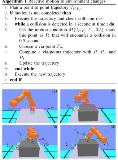
Algorithm 1 Reactive motion to environment changes
1: Plan a point to point trajectory TPiPf
2: if motion is not completed then
3: Execute the trajectory and check collision risk
4: while a collision is detected in 1 second at time t do
5: Get the motion condition M (TPiPf, t + 0.5), mark this point as Pc that will encounter a collision in
0.5 second
6: Choose a via-point Pm
7: Compute a via-points trajectory with Pc, Pm and
Pf
8: Update the trajectory
9: end while
10: Execute the new trajectory
11: end if
Fig. 6. A simulated move form an initial position to an final position with a static obstacle. The purple dashed line is the trajectory computed in advance. The green solid line is the real path which the robot follows. By adding two way points, the robot reaches the target position without collision and path replanning at the high level.
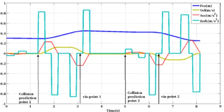
Z axis. The position curve shows how the trajectory deviate from the pre-planed one (straight line from the initial position to the final position) due to the predicted collision risk. In the first four segments, the executed trajectory coincides with the pre-planed one. At the collision prediction point 1, the system switches to a new trajectory. The smooth velocity profile shows that the trajectory transition is instantaneous and continuous.
The computation for this Cartesian space trajectory with 6 via-points requires an average execution time of 1.2 ms on a Intel Core(T M )2 Quad CPU 2.66GHz machine. It is fast enough for real time applications, such as visual servoing or reactions to other sensor events.
B. Robot Experiments
We also implemented the via-points trajectory generator on a KUKA light-weight robot IV [16], which was controlled through the Fast Research Interface [17]. The software control is developed using Open Robots tools: GenoM [18].
Fig. 7. The position, velocity, acceleration and jerk of online generated via-points trajectory on Z axis
Fig. 8. Paths of the robot end effector with different Ev
The sampling time is fixed to 10 ms. The Pose of the manipulator’s end effector is defined by seven independent Operational Coordinates. It is composed of a position vector P = [x, y, z]T and by a quaternion Q = [n, q]T, where q = [i, j, k]T. They give the position and the orientation of the final body in the reference frame. The linear and angular end-effector motion bounds are given in table I.
TABLE I
ROBOT MOTION IS LIMITED IN JERK,ACCELERATION,AND VELOCITY
Jmax Amax Vmax Linear limits 0.900 m/s3 0.300 m/s2 0.150 m/s Angular limits 0.600 rad/s3 0.200 rad/s2 0.100 rad/s
Fig.8 illustrates the the same path of the robot end effector as in the previous simulation. δ = 1.0 means the smoothed trajectory starts at the end of maximum velocity segment. While δ = 0.8 means the start points are closer to the intermediate points, which results in a smaller error. The straight-line path is a path with zero error, which can be represented by defining δ = 0.
VII. CONCLUSIONS ANDFUTURE WORKS
This paper proposed a solution to generate trajectories defined by via-points and a parameter defining the size of the smoothing area. Using projection of constraints, it can build trajectories in Cartesian space. Due to direct computation
without optimization computation or randomized algorithms, the proposed solution takes short execution time and is able to be used online. Experimental results show the validity of the approach for real-time control, especially for online collision avoidance. We are going to integrate the via-points generator for realizing a real reactive manipulation. It would also be interesting to introduce the kinematic model to take into account both joint and Cartesian constraints. New solutions for fixed time trajectory generation can be proposed.
REFERENCES
[1] T. Flash and N. Hogan. The coordination of arm movements: an ex-perimentally confirmed mathematical model. Journal of neuroscience, 1985.
[2] Jingyan Dong, PM Ferreira, and JA Stori. Feed-rate optimization with jerk constraints for generating minimum-time trajectories. Interna-tional Journal of Machine Tools and Manufacture, 47(12):1941–1955, 2007.
[3] A Zabel, H M¨uller, M Stautner, and P Kersting. Improvement of machine tool movement for simultaneous five-axes milling. In CIRP international seminar on intelligent computation in manufacturing engineering, pages 159–64, 2006.
[4] T. Kr¨oger. On-Line Trajectory Generation in Robotic Systems, vol-ume 58 of Springer Tracts in Advanced Robotics. Springer, Berlin, Heidelberg, Germany, first edition, jan 2010.
[5] L. Biagiotti and C. Melchiorri. Trajectory Planning for Automatic Machines and Robots. Springer, November 2008.
[6] Alessandro Gasparetto, Paolo Boscariol, Albano Lanzutti, and Renato Vidoni. Trajectory planning in robotics. Mathematics in Computer Science, 6(3):269–279, 2012.
[7] S. M. LaValle and J. Kuffner. Rapidly-exploring random trees: Progress and prospects. In Workshop on the Algorithmic Foundations of Robotics, 2001.
[8] L´eonard Jaillet and Thierry Sim´eon. Path deformation roadmaps: Compact graphs with useful cycles for motion planning. The Interna-tional Journal of Robotics Research, 27(11-12):1175–1188, 2008. [9] L´eonard Jaillet, Juan Cort´es, and Thierry Sim´eon. Sampling-based
path planning on configuration-space costmaps. Robotics, IEEE Transactions on, 26(4):635–646, 2010.
[10] Santiago Garrido, Luis Moreno, and Dolores Blanco. Exploration of a cluttered environment using voronoi transform and fast marching. Robotics and Autonomous Systems, 56(12):1069–1081, 2008. [11] Xavier Broquere, Daniel Sidobre, and Ignacio Herrera-Aguilar. Soft
motion trajectory planner for service manipulator robot. Intelligent Robots and Systems, 2008. IROS 2008. IEEE/RSJ International Con-ference on, pages 2808–2813, Sept. 2008.
[12] Daniel Sidobre and Wuwei He. Online task space trajectory genera-tion. In Workshop on Robot Motion Planning Online, Reactive, and in Real-time, 2012.
[13] Hongyao Shen, Jianzhong Fu, and Zhiwei Lin. Five-axis trajectory generation based on kinematic constraints and optimisation. Inter-national Journal of Computer Integrated Manufacturing, (ahead-of-print):1–12, 2014.
[14] A.Frisoli, C.Loconsole, R.Bartalucci, and M.Bergamasco. A new bounded jerk on-line trajectory planning for mimicking human move-ments in robot-aided neurorehabilitation. Robotics and Autonomous Systems, 2013.
[15] X. Broqu`ere and D. Sidobre. From motion planning to trajectory control with bounded jerk for service manipulator robots. In IEEE Int. Conf. Robot. And Autom., 2010.
[16] KUKA Roboter GmbH. http://www.kuka.com/en/company/ group.
[17] G. Schreiber, A. Stemmer, and R. Bischoff. The fast research interface for the kuka lightweight robot. In Proc. of the IEEE ICRA 2010 Workshop on ICRA 2010 Workshop on Innovative Robot Control Architectures for Demanding (Research) Applications - How to Modify and Enhance Commercial Controllers, pages 15–21, 2010.
[18] R. Chatila S. Fleury, M. Herrb. Genom: A tool for the specification and the implementation of operating modules in a dist ributed robot architecture. In EEE/RSJ International Conference on Intelligent Robots and Systems, pages 842–848, 1997.