Efficient Customization of Coaxial Offset Shoulder Grinding
by
Andrew J. Laures
B.S. Mechanical Engineering (1995) Massachusetts Institute of Technology
SUBMITTED TO THE SYSTEM DESIGN AND MANAGEMENT PROGRAM IN PARTIAL FULFILLMENT OF THE REQUIREMENT FOR THE DEGREE OF
MASTER OF SCIENCE IN ENGINEERING AND MANAGEMENT
AT THE
MASSACHUSETTS INSTITUTE OF TECHNOLOGY June 2000
@ 2000 Massachusetts Institute of Technology All Rights Reserved.
Signature of Author
Syste>'sign and Management Program January 1 th, 2000
Certified by
Daniel D. Frey Thesis Advisor Professor of Aeronautics & Astronautics
72 ,I
Accepted by
Thomas A. Kochan LFM/SDM Co-Director George M. Bunker Professor of Management
Accepted by
Professor of Aeronautics & Astronautics
MASSACHUSETTS INSTITUTE OF TECHNOLOGY
FEB
1
o
2000
Paul A. Lagace LFM/SDM Co-Director and Engineering Systems
Abstract
Mechanical Grinding is a complicated art packaged in a deceptively simple technique. The analysis presented here attempts to unravel some of the mystery by proposing a mathematical model to describe the interface between the grinding wheel and the workpiece in Coaxial Offset Shoulder Grinding. The goal is to better understand the geometry of this interface as a function of the alignment of the axes of rotation of the two wheels. By iterating the model with different initial conditions, an
optimal configuration might be found which describes a situation providing for a minimized peak rate of wear across the grinding wheel. Examples using the model have shown a reduction of more than 2 orders of magnitude in the peak rate of wear, a situation which would drastically improve the process efficiency, by reducing the frequency of wheel dressing, and enable a higher effective material removal rate. The tangible benefit of the model would be its use as a simulation tool in industry to facilitate the task of optimizing a grinding process. Depending upon the process and the company, it is estimated that by using simulation, rather than prototyping, as a testbed, development costs can be reduced by more than $100,000 and leadtimes can be a couple of hours instead of several months. In addition to these up-front savings, the resulting process will most likely result in more efficient manufacture and higher quality.
1.0 Introduction
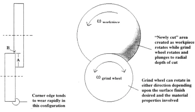
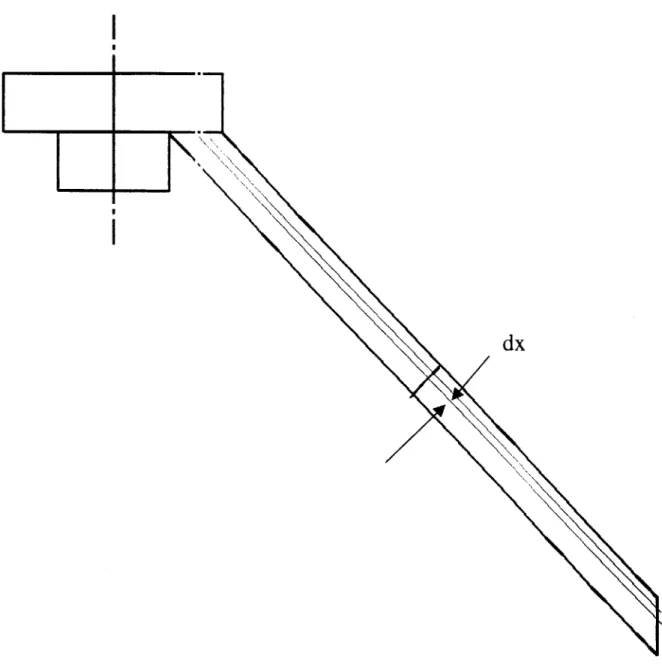
This thesis documents the analysis conducted to understand the effective geometry of the grinding wheel cutting face and the associated mathematical model developed to calculate the Material Removal Rate (MRR) as a function of location on this surface. The impetus for this effort was the discovery, from experience and experiment in industry with the Coaxial Offset Shoulder Grinding Process (See Figure 1), of two interesting phenomena. Using these discoveries, the peak rate of wear experienced by the grinding wheel can be reduced while at the same time enabling an increase in the overall Material Removal Rate capacity, both without changing the material properties or the rate of rotation of either the grinding wheel or the workpiece.
.1
A
Corner edge tends to wear rapidly in this configuration
grind wheel 1
/
"Newly cut" area created as workpiece rotates while grind wheel rotates and plunges to radial depth of cut
Grind wheel can rotate in either direction depending upon the surface finish desired and the material
properties involved
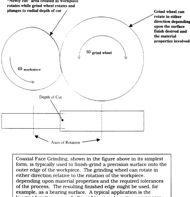
Figure 1: Coaxial Offset Shoulder Grinding
The complete history of the experiments conducted in industry that contributed to the public knowledge of the two phenomena investigated in this thesis would be quite long and complicated. Considering the age (over 40 years old) of some
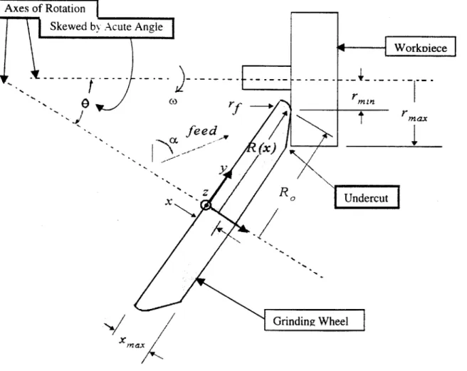
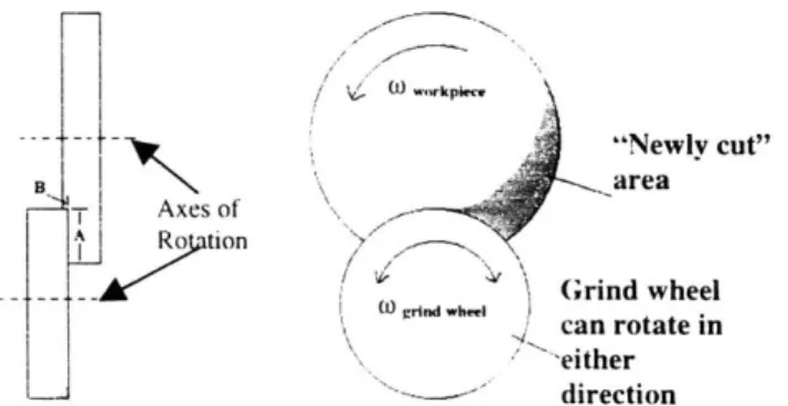
of the patents describing the use of these phenomena in grinding applications, it is clear that at least an awareness of them has been around for a long time. The investigation described herein was motivated not to simply continue this history, but instead to better understand recent experiments conducted at Landis Gardner 1. a manufacturer of grinding equipment and accessories. These two key phenomena upon which the model is based are, specifically, the introduction of a *skew angle" so that the axes of rotation of the grinding wheel and workpiece are no longer parallel, and the use of an "undercut" on the side of the grinding wheel next to the shoulder face of the workpiece (See Figure 2).
Axes of RotationII
Skewed by Acute Angle
IWorktoieceI min max f eed~ X R Undercut Grinding Wheel x
Figure 2: Key Phenomena Represented in Model (red)
The development of the mathematical model was requested by representatives of Landis Gardner in an effort to better understand their experimental findings and to possibly enable the development of better grinding machines and/or grinding processes. The Landis-Gardner representatives were interested in elevating the knowledge level of these phenomena from an awareness to a thorough understanding.
Page 4 of 51
The "undercut" helps to prevent the side of the wheel from rubbing against the shoulder face of the workpiece. While the geometry of the traditional setup suggests that the contact should not happen, power requirements for the process indicate otherwise. As is later discussed, Thermal Expansion is
involved. The "skew angle" significantly alters the geometry and kinematics of the contact area between the grinding wheel and the workpiece. The result is a significant reduction in the peak rate of wear experienced by the grinding wheel. Correspondingly, the mathematical model creates a geometric representation of the cutting surface based upon the several parameters affected by the changes. It is important to note that, while the nominal geometry of the grinding wheel changes, the net effect on the nominal geometry of the finished workpiece remains unchanged. Only the process itself is affected by the changes, not the output thereof.
While the results 2 accumulated during the long history of industrial
experiments in this area were only capable of providing qualitative information on the effects of their respective changes in the process parameters, they were quite beneficial. For example, the empirical data indicated that the "undercut" would result in a reduction in the grinding wheel power consumption and, consequently, the workpiece temperature. Everything else remaining the same, the corresponding decrease in the temperature gradient across the workpiece results in a better surface finish quality. 3 Historical trials conducted with a machine layout modified with the "skew angle" showed a significant reduction in the peak rate of wear experienced by the grinding wheel. Significantly, while the findings from both of these experimental modifications were unable to
quantify their respective benefits, they were still important enough to patent. 4
2 Because of the age of the information to which I am referring, and the widespread awareness and application of it in the grinding industry, it is considered in the context of this thesis to be "common knowledge." The use of specific references might detract from the universality of the example.
3 Shaw, Milton C. Principles of Abrasive Processing pp. 261-313. Chapter 10, entitled "Surface Integrity," addresses several of the effects of grinding temperature on surface finish. The main focus of the chapter is to point out that it is very beneficial to keep the temperature as low as possible to enable higher quality control.
4 United States Patent #4115958, "Method of Cylindrical and Shoulder Grinding," protects just about every possible
scenario resulting from these findings. No mention is made of any specific benefits, but the patent basically protects the use of these layout changes in any combination, thereby allowing the patent holder to experiment further and effectively customize a given process with trial and error.
Looking only at the investigations pursued in this thesis, the goal of the analysis leading up to and including the creation of the mathematical model was to bring to fruition the capability of generating instead a quantified
measurement of the beneficial effects of the changes. A literature search revealed that this capability would offer a unique level of understanding of the system. It was hoped that, aided by the ability to calculate quickly and easily the optimal setup parameters, processes could now be customized to the specifics of the task at hand rather than only loosely adapted to the new
conditions with the help of a vague understanding of cause/effect relationships.
A thorough description of the equations in the model is provided in Section 3.2
since understanding the inner workings of an analytical tool is one of the better ways of learning how to best take advantage of the functions it offers. Section
3.3 contains graphs generated by the simulation tool for various "skew angle"
and "direction of grinding wheel movement" parameters. Each iteration is briefly detailed and a discussion developed regarding the best combination.
A model is only applicable if its output is consistent with observations in the
physical world. Because the mathematical model was motivated by and based upon physical tests, and the data from these tests was readily available, it was very easy to test the output of the model. The data from these physical tests have confirmed the validity of the trends described by the model.
2.0 Background
The technique of using one object which is abrasive, and relatively harder, to remove material from another object has been known and used for literally thousands of years. This simple technique, or art, is called Grinding. The ancient Egyptians relied upon it to shape the blocks they used in their pyramids and the Incas used it to build magnificent, mortar-less structures that still stand today. 5 It probably will not come as a surprise, however, that modern industry needs a much more thorough understanding of the technology than these cultures ever had. Today we find that "the application of
superabrasives and increasing demands for higher productivity and higher
quality require an appropriate selection of optimum set-up parameters." 6
Knowing what these optimal parameters are demands a more thorough
understanding of the interface between the workpiece and the grinding wheel.
2.1 The Industrial Perspective
Industry often relies upon grinding to achieve high tolerances and/or difficult geometries. Because grinding wheels are typically made of materials that are very hard, the cutting surface can be controlled to extremely tight tolerances, even into the sub-micrometer range. 7 This level of control, however, demands that the geometry of the grinding wheel cutting face does not change
significantly. Wear will occur of course, but the rate and location of this wear, more than just its existence, are what is important.
Based upon the experience gained over time while using a process, the grinding wheel will be resurfaced, or "dressed," after a predetermined number of cutting cycles in order to reestablish a baseline. At this point. the machine again "knows" exactly where the cutting edge is in relation to the workpiece. Depending upon quality controls and the conditions experienced with the process, dressing might be scheduled every 100 cycles, for example, or every
1,000 cycles, etc. In extremely precise operations, the wheel might be dressed
every cycle. It all depends upon what is required for the specifics of the process and product.
While dressing the grinding wheel is great for quality control, it has a major drawback. It is entirely unproductive. Dressing the grinding wheel uses machine time, significantly accelerates the wheel wear, and requires the use of an expensive diamond tool which has a limited lifecycle. Identifying the optimal parameters that will increase the number of cutting cycles between dressings is therefore of great importance for increasing productivity and reducing cost.
5 Based upon the author's recollection of scientific explorations of these cultures as presented on Public Broadcasting System programming.
6 Warnecke & Zitt, University of Kaiserslautern: excerpt from CIRP Annals - Manufacturing Technology v47 nl 1998, Hallwag Publishers, Ltd.: Berne, Switzerland. P265-270 [0007-8506 CIRAATJ
Laures
Many advances have been made to improve the wear life of grinding wheels, but it seems that little effort has been made to find the root cause behind the
accelerated wear typical of certain areas of the grinding wheel. 8 In some
applications, a stress concentration due to the geometry at the interface may be the reason behind rapid wear of a portion of the cutting surface. In many other applications, however. it might instead be that the area of concern is required to remove a majority of the material from the workpiece. 9 The analysis in this investigation concentrates upon mitigating the effects of this second scenario primarily by helping the users of a process to identify or verify that an MRR concentration is the cause of the accelerated wear. If the wheel geometry and/or the machine layout can be adjusted to reduce this peak wear rate without affecting the desired part geometry, then the number of cycles between dressings can be significantly increased. Process efficiency will benefit from a reduction in this inherent downtime.
2.1.1 Quality Control and Material Removal Rate
Industrial processes often involve a compromise. Meeting part specifications typically comes at the expense of productivity. The goal is therefore to meet the constraints while maximizing output. This same struggle exists in Mechanical Grinding where the specification involves surface finish quality and the struggle is to maximize the MRR so as to require the minimum processing time while also taking into consideration the downtime required for dressing the wheel. The contributing factors to surface finish quality in grinding are numerous and
highly coupled. 10 The speed with which the grinding wheel surface traverses the workpiece is an example. 11 Therefore, a change that improves the MRR but
does not alter the speed of the grinding wheel surface would be desirable since 7 Shaw, Milton C. Principles of Abrasive Processing pp.
452-3.
8 Based upon the appearance. from the literature search, that the model presented in this thesis is unique.
9 As is later discussed in the next Section, the rate of material removal demanded of a grinding wheel, or a section thereof, determines how quickly wear will occur at the location being considered.
'0 Shaw, Milton C. Principles of Abrasive Processing pp. 261-313. Consult Chapter 10, entitled "Surface Integrity," for a detailed and comprehensive discussion of the effects upon surface finish.
" Shaw, Milton C. Principles of Abrasive Processing pp. 266-7. The "First order Interactions" in Table 10.2 on page 266 and in Table 10.3 on page 267 both demonstrate the heavy coupling associated with the "work speed" which is the speed (in feet per minute, f.p.m.) with which the surface of the grinding wheel traverses the workpiece.
Laures
it does not automatically affect the coupled contributions to surface quality. The simulation tool promotes changes that do not affect wheel speed.
Assuming that a Coaxial Offset Shoulder Grinding process has been
incrementally improved over time, it is fair to assume that the ratio of the MRR (as determined by the infeed rate and workpiece grinding wheel surface speed) to the number of dressing cycles per, for example, 1,000,000 parts, has already been maximized. This considered, the process cannot be improved by simply
increasing the infeed rate and spinning the wheel faster. These options have already been optimized. Instead, the kinematics of the interface between the grinding wheel and the workpiece might be altered to effect a beneficial change
in the ratio by increasing the MRR capacity, by reducing the rate of dressing cycles. or both. The changes promoted by the simulation tool actually do both. Historically, the most common approach to increasing the MRR had been to simply turn the grinding wheel faster. The primary determinant of the grinding wheel maximum RPM is the material from which the wheel is made. 12
Correspondingly, significant advances have been made in grinding wheel materials properties. As a result, modern grinding wheels spin at speeds even two orders of magnitude faster than they did fifty years ago.
It is important to note, however, that grinding wheel RPM and actual MRR are not precisely correlated. Pushing a grinding wheel toward its maximum RPM only serves to significantly increase the rate of wear disproportionately to the increase in the amount of material being removed. 13 Brittle fracture of the
wheel under these extreme conditions occurs more readily. Consequently, most grinding wheels used in production environments typically run at about
85-90% of maximum RPM. 14 In this way, overall productivity is kept high. The 12 This is the case when considering the same workpiece material since changing the workpiece material affects the
maximum desirable grinding wheel RPM. When grinding Titanium alloys, for example, the grinding wheel speed should be about one-third that used in conventional grinding applications. This specific example is cited in Shaw, Milton C. Principles of Abrasive Processin , page 326.
13 The dynamics affecting the wear of the grinding wheel are numerous and impressively complicated. Milton Shaw does a great job to detail most or all of the contributing effects. Refer specifically to pp. 54-81, 315-244, 403-9 in Shaw, Milton C. Principles of Abrasive Processing for explanations of the majority of these effects.
goal, therefore, is to arrive at a means of achieving a relatively higher MRR while still keeping wheel deterioration under control.
2.2 First Look at the Proposed Method
Reflecting upon the background just provided, the direction taken in this thesis seems almost obvious. Moving away from the "coaxial approach" of using parallel axes of rotation for the grinding wheel and workpiece (See Figure 3) geometrically enables an increase in the contact patch area and, in effect, a
reduction in the peak rate of wear experienced by the grinding wheel. As was also discussed, if the contact patch area per unit time is increased, the MRR will similarly increase. Consequently, the total productivity for a grinding
process can be improved significantly without the need for anything more exotic than a differently shaped grinding wheel and a realigned arbor.
"Newly cut" area
-T Axes of
A R tion
"Newly cut" area
grind wheel Grind wheel
can rotate in either
direction
Coaxial Offset Shoulder Grinding
Grind heel can rotate in either
grind wrheel direction (wnwkpkce
Depth f Cut
V'Axes of Rotation
Coaxial Face Grinding
Figure 3: "Coaxial" Grinding Examples
The real breakthrough in this new process is the quantifiable understanding of the geometric intricacies at the interface between the grinding wheel and the workpiece. By mathematically modeling this interaction, it is possible to compute the maximum MRR as a function of the modified imposed geometry.
The only special requirement is the departure from the "standard" design used for a grinding wheel in coaxial grinding. Instead of working with what is
typically a symmetrical wheel, the new grinding wheels, mounted with an introduced angle between the arbor and workpiece, will have a specially contoured face that counteracts the effect of the introduced angle.
2.2.1 Coaxial Offset Shoulder Grinding
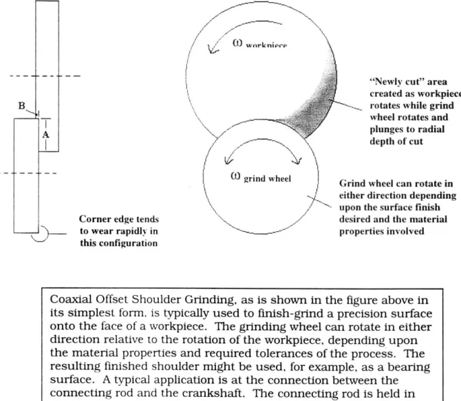
As was already detailed. the mathematical model developed in this thesis has been specially tailored for application to the Coaxial Offset Shoulder Grinding process (See Figure 4). This process is most often used to put the finishing touches on the critical surfaces of shoulder bearings. Industrial experience demonstrates that most of the wear during Coaxial Offset Shoulder Grinding occurs at the extreme outer edge of the grinding wheel (again, refer to Figure 4). Intuition might dismiss this phenomenon as simply consistent with the edge being the most fragile point on the wheel. Studying closely the kinematics of the situation reveals instead that this edge is actually required to do most of the material removal and is therefore subject to the most rapid wear. Even though a larger portion of the grinding wheel (Sections A & B in Figure 4) appears to be in contact with the workpiece, only the small portion that is at the corner edge (Section B in Figure 4). actually removes the depth of cut of the material. The remaining portion (Section A in Figure 4) in contact with the workpiece does very little if any cutting. Geometrically, the only cutting Section A should be required to do would be any material left behind as the corner edge wears from its original dimensions.
kr'
rknipri-rind wheel
"Newly cut" area created as workpiece
. rotates while grind wheel rotates and plunges to radial depth of cut
Grind wheel can rotate in either direction depending upon the surface finish desired and the material
properties involved
Figure 4: Coaxial Offset Shoulder Grinding
Unfortunately, Thermal Expansion complicates the simple geometric model created to understand Coaxial Offset Shoulder Grinding. As heat is generated during the grinding process, thermal expansion of the workpiece brings the cut surface into contact with Section A of the grinding wheel. Assuming that the
Page 12 of 51 B
A
Corner edge tends to wear rapidly in this configuration
Coaxial Offset Shoulder Grinding, as is shown in the figure above in its simplest form. is typically used to finish-grind a precision surface onto the face of a workpiece. The grinding wheel can rotate in either direction relative to the rotation of the workpiece, depending upon the material properties and required tolerances of the process. The resulting finished shoulder might be used, for example, as a bearing surface. A typical application is at the connection between the connecting rod and the crankshaft. The connecting rod is held in place by the shoulders on either side so they must be smooth to reduce friction. In the case of a crankshaft, the grinding wheel would also finish the main bearing surface in addition to the shoulder. In the figure, this bearing surface would simply be an extension of Section B on the part beyond the depth of cut on the shoulder surface denoted by Section A.
corner edge of the grinding wheel has not worn substantially, the thermal expansion usually generates only enough force to cause significant friction but no material removal. 15 The allowance in the model for an "undercut" has been made to account for this expansion and to negate its detrimental effects. In addition, the added space between the grinding wheel and the shoulder face of the workpiece allows for better coolant access to this area.
3.0 Developing the Mathematical Model
Prior to the analysis made in this thesis. experiments conducted in industry had revealed that the wear at the corner edge of the wheel in Coaxial Offset Shoulder Grinding could be reduced by introducing an angle (the "skew angle") between the axis of rotation of the arbor and that of the workpiece. The next step, which is where this thesis begins, was to understand the kinematics driving these experimental results. A mathematical model was chosen for this task since it would enable the complex interaction to be broken down into its constituent parts. These parts could, it was hoped, be individually understood and modeled more easily than the whole. As an added bonus, a mathematical model would also allow for the situation to be generalized and then optimized for any given set of conditions.
As a first step in understanding the mathematics involved with modeling the system, a cursory approach was taken to describe the simpler system of "Coaxial Face Grinding" (See Figure 5). Coaxial Face Grinding is similar to Coaxial Offset Shoulder Grinding in that the grinding wheel and workpiece are rotating about parallel axes. The interface between the workpiece and the wheel in the former, however, is much simpler and provided good insight into mathematically modeling the MRR. Once this scenario was understood, the technique was applied to Coaxial Offset Shoulder Grinding. Next, the concept of an introduced angle between the axes of rotation of the workpiece and the grinding wheel (See Figure 6) was included in the analysis, proving that wear to
15 For a thorough discussion of the effects of Thermal Expansion in a grinding process, consult Parts I & II of
"Contact Length in Grinding" by Qi, Rowe, and Mills. These reports, from pp. 67-85 of the "Proceedings of the Institution of Mechanical Engineers. Part J": Journal of Engineering Tribology v21 1 ni 1997, describe the
the edge of the grinding wheel could be significantly reduced by increasing the effective cutting edge surface area. Finally, a provision was included in the model to allow for an "undercut" on the grinding wheel (See Figure 7) which eliminates the drag caused by Thermal Expansion. This final step completed the imitation of the physical model developed by Landis-Gardner.
"Newly cut" area created as workpiece rotates while grind wheel rotates and piunges to radial depth 01 cut
Depth of Cut
~.1~
Grind wheel can rotate in either direction depending upon the surface finish desired and the material properties involved grind wheel / / / / 7 -7 Axes of Rotation
Figure 5:
Coaxial Face Grinding
Coaxial Face Grinding. shown in the figure above in its simplest
form, is typically used to finish-grind a precision surface onto the
outer edge of the workpiece. The grinding wheel can rotate in either direction relative to the rotation of the workpiece,
depending upon material properties and the required tolerances of the process. The resulting finished edge might be used, for example, as a bearing surface. A typical application is the bearing locations on a shaft used in an automotive compressor. The depth of cut for this shaft application is about 150 microns.
Axes of
xes o
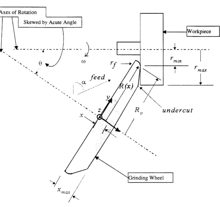
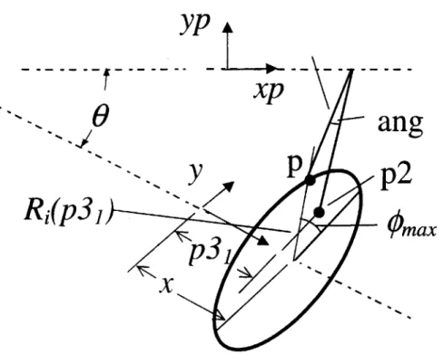
Figure 6: Acute Angle Added to Coaxial Offset Shoulder Grinding
Page 16 of 51
Rotation
Skewed by Acute Angle r in r
m ax
ex
'IP 0 r WorkpieceYR
R
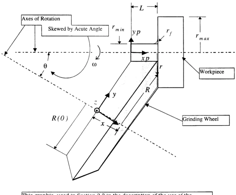
(0) Grinding Wheel xThis graphic, used in Section 3.3 in the description of the use of the simulation tool, shows very well what is meant by the introduction of an acute angle between the axes of rotation of the grinding wheel and the workpiece. The angle used in most applications would not be as large as is shown, but could be if needed. The take-away from this concept is the huge reduction in peak wear rate resulting from the introduction of even only a very small angle. The graphs in Section 3.3 demonstrate this fact.
r
rf
feed
z
R
und
Grinding Wheel ,fljfercut
The figure above shows a further specialization of Coaxial Offset Shoulder Grinding. Here an "undercut" has been added to the portion of the wheel which otherwise would be directly next to the shoulder face of the workpiece. Experiment in industry has shown that the presence of this undercut significantly reduces the power required to drive the grinding wheel, suggesting that this area otherwise rubs against the shoulder face even though geometrically it should not. As is discussed, Thermal Expansion is involved. The model has been designed to accommodate this undercut in order to take advantage of the power savings while modeling accurately the MRR.
Figure 7: Undercut Added to Coaxial Offset Shoulder Grinding
xes of Rotation
Skewed by Acute Angle
r
max0
N
nmaxX
3.1 Motivation Behind a Generalized Case
Of course, this modeling venture was not just an intellectual detour into the
realm of mathematics without awareness of a broad industrial application. While a simpler model might have been developed to explain the results seen in the industrial experiments, the real payoff was in making a model that could be used to understand and optimize any process.
Applying the method of using an introduced angle in the Coaxial Offset Shoulder Grinding process basically increases the cutting area seen by the workpiece. Consequently, the processing time for a given operation can be
reduced significantly and the number of grinding cycles between wheel dressing cycles can be increased since now the critical cutting face is not wearing nearly as quickly. The potential for an increase in the MRR, coupled with the
reduction in required wheel maintenance, enables productivity improvement without the need for significant changes in either the machine or the tooling.
Interestingly, however, the effect of these changes on the Overall Equipment Efficiency (OEE) for the process can be positive, negative, or nonexistent (See Section 4.1 for a thorough explanation of this apparent ambiguity). This uncertain impact on the OEE is very important to note. Depending upon the managerial philosophy at a plant, a process might be bound by the OEE measurement without a thorough understanding of the effects of proposed changes upon the overall productivity of the process.
The introduced angle does require some reconfiguration of the grinding
equipment. which might be expensive. However, since the technique does not require the use of an entirely new technology, it is much easier and more cost effective to implement than another approach which might introduce an entirely new process.
3.2 Constructing the Mathematical Model
In this section, I develop an algorithm for computing material removal rate in thrust wall grinding as a function of key processing parameters. The
parameters of the process are depicted in Figure 6 and are explained below:
8 -- The angle between the workpiece axis of rotation and the grinding wheel's axis of rotation. The two axes are assumed to lie in the same plane. In this model, the plane that contains both axes is defined to be the x y plane.
a-- The angle at which the grinding wheel feeds into the part (see Fig. 7)
w - The rate of rotation of the workpiece as it is driven by the workpiece spindle.
r,,,, - The smaller radius of the two cylindrical sections comprising the
workpiece. This section of the workpiece undergoes cylindrical grinding.
r,, - The larger radius of the two cylindrical sections comprising the workpiece. The planar section of the workpiece on the face of the larger cylinder undergoes thrust wall grinding.
r,- The fillet radius at the corner between the cylindrical part of the workpiece and the thrust wall.
L - The axial length of the smaller cylindrical section of the workpiece whose radius is rm,.
R(x) - The radius of the grinding wheel as a function of axial position. This radius must be defined by the user at least one location. In this model, the user must define R(O), the radius at the origin of the xy coordinate system. This coordinate system origin is set at the left edge of the grinding wheel which is aligned with the left edge of the workpiece.
d -- The depth of cut as defined by the total amount of grinding wheel infeed per
full revolution of the part.
Given the inputs described above, one may compute the value of x at the right face of the grinding wheel
X max := Lcos(e) + (r max- r mm) sin()
And given this parameter, one may define a function describing the shape of the grinding wheel. This is defined via a function of axial position R(x).
R(x) R 0 - x-tan(90 -deg - 0) if x < 0
R 0 + x-tan(0) if 0 5 x < iL - r f)-cos(O)
if [(L - r f) -cos(O) 5 x] < L-cos(O) + r .si(O) + r -tan(undercuo -sii(8)
R O + ( L- r r) sini4O - r f-cos(O) +4r,2 -[x - (L - rf) -cos(O) - r,. si40) o
I
(R0 + L-sin(8)) - (x - Lcos(O)-(tan(90-deg - 0)) if L-cos(0) + r -sin(O) X < X max [[R + L sin(O) - (x - L-cos())-tan(90-deg - 0) + (x - X max)-tan() ]if X max 5 X
The grinding wheel is a surface of revolution constructed by revolving this curve R(x) about grinding wheel's axis of symmetry (the x-axis). The final shape of the part will be the same curve revolved about the workpiece axis of symmetry (the
xp-axis) (see Figure 6).
For the algorithm to work. one must also define the shape of the part before the grinding process began or the part's shape after the last pass of the grinding wheel (whichever is appropriate in the given context). This is essential in
computing MRR because the material that is to be removed is bounded between the surfaces defining the workpiece before and after grinding. I assume that the shape of the part before grinding is formed by displacing the grinding wheel profile a distance "d" parallel to the direction of infeed as defined by the
parameter a. The shape from the point of view of the grinding wheel axis system is given by
R i(x) R,, - x-tan(90-dcg - o) if x < d-cos(a) -sin(6)
otherwise
R(x- d-sin(9 - C)) - d-cos(O - x) if [x < x max- d-sin(a)-(cos(O))]
R, ,+ Lsin(O) - (x max - L-cos())-tan(90 -deg - 0) + (x- xma).tan(9)]] otherwise
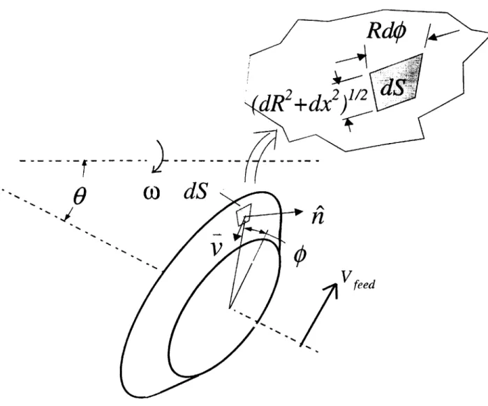
With the geometry of the grinding process described mathematically, it should now be possible to compute the material removal rate (MRR) experienced by the grinding wheel at any location. To understand the approach taken, it is useful to study Figure 8 which depicts a differential element on the surface of the grinding wheel. Let us assume that this surface element lies within the grinding zone and that the differential element lies within a section of the grinding wheel a distance x from the origin above the xy plane by an angle 0.
dR
2+dx
2 1 2dS;.
0)
dS
V
'pb
Vfeed
Figure 8: A differential element on the surface of the grinding wheel.
Due to the rotation of the workpiece and the infeed of the grinding wheel,
material is flowing across the boundary of the differential element. The velocity of the flowing material with respect to the grinding wheel is
V cox r+ V feed
where r is the shortest vector from the workpiece axis to the differential element. This vector r can be described in terms of input parameters as
RO rmin
tan(O) sin(o)
R(x)-cos($) R(x).-sin(o)
Since the workpiece is at an angle 0 to the grinding wheel, the vector describing the workpiece rotation is
(0-cos(e)
o
=msin(6)I
0
Similarly, the vector describing the infeed velocity can be described in terms of input variables ---. d-sin a - 0) 2-7r V feed= dcos(c -O) 2 -i 0
Now, the total flux of material across the element is given by the cross product of the velocity and the unit normal to the surface times the area of the
differential element. The unit normal to the surface is
-si at R(x)
cos ata d R(x) -).cos(o)
dx A
The area of the differential element is simply the product of the length of its sides. The length of the side in the direction of the sweep about the grinding wheel axis is simply Rd4 (see Fig. 8). The length of the side in the axial direction is not simply dx because the surface of the grinding wheel may be at an angle to the axis of symmetry of the grinding wheel - dR/dx is not zero in general. So, the length of that side is the square root of the sum of dR2 and dx2. So. the flux through the differential element is
FLUX= n.v.R(x)- 1 + R(x)Y])
Lx x ,
In order to understand why certain sections of the grinding wheel (as defined by axial location) wear more quickly than others, we wish to compute the MRR as a function of axial location x. This can be computed by taking slices of the grinding wheel defined by two planes perpendicular to the grinding wheel axis of symmetry. The planes are at axial position x and are separated by a small distance dx (see Figure 9).
dx
Figure 9: A differential "slice" of the grinding zone.
In order to compute the total MRR for that slice, one only needs to integrate the flux within the grinding zone. As it is defined in Figure 8, the grinding zone
begins at an angle $=0 where the final shape of the workpiece and the grinding wheel are tangent. Let us call the angle at the upper end of the grinding zone
$ma(x). This angle is in general a function of x - as axial position changes, the width of the grinding zone may change. In general, the material removal rate as a function of axial position is therefore
MRR(x = -()
n-v-R(x)- I+ Rx d$ dx
(d_
For certain special cases of workpiece geometry it is possible to compute a closed form solution for $a(X). However, I wish to provide a solution method that can accommodate the general case that the grinding wheel geometry is defined by a function R(x. In this case it is possible to compute (.(x) using a root finder 0 inax(x) := root(Dif1($,x),O) where Dift($,x) := p +- T R(x)-cos($) R(x)-sin($) ang <-- -at -4P2) 1 0 0
p2+-- 0 cos(ang) -sinaang) i-p
0 sin(ang) cos(ang)
)
p3 <- Tinx(p2)
R i(p31) - p32
This approach is best understood by considering Figure 10. Point p is a point within the differential slice at an angle $ from the xy plane about the grinding wheel axis of symmetry. If this point is at the top of the grinding zone, then it
should lie on a surface of revolution formed by rotating the radius of the uncut part Ri(x) about the workpiece axis of symmetry. This can be determined by the following procedure:
* Express point p in terms of the workpiece coordinate system - the operator T() transforms the coordinates in the appropriate way.
(cos(O) Sirq) 0 ) R o0sin(0)
T(p) := -sin(8) cos(e) 0 -p - r min+ R -cos(e)
0 0 1 ) 0
* The angle of the point p above the xv plane about the workpiece coordinate system, "ang-, can be computed using the arctangent operator.
* Rotate the point p by -ang about the workpiece axis of symmetry so that it lies in the xv plane. This gives the coordinates of the point p2 expressed on the xp
yp frame
* Transform the point into the grinding wheel coordinate system using the inverse transform to yield the coordinates of p2 expressed in the xy frame. These coordinates are assigned the label p3
cos(e) -sin(O) 0
[
RO-sin(0)TinV p) sin(O) cos(O) 0 p + rmin+ Ro -cos(O)
S 0 1
* If the value of o sent as an argument to the function Diff is at the top of the grinding zone, then the y coordinate of point p3 should be equal to the radius of the uncut part evaluated at the x location of that point, Rj(p31) should
equal p32
* A search using a root finder for a point where the function Diff is zero will yield the value of $ at the top of the grinding zone. This is the value needed as the upper limit of integration in the integral defining MRR(x).
yp
xp.
0
ang
Yp
p2
Ri~p33
Vmax
Figure 10: Solving for the limits of the grinding zone.
The algorithm described above will allow one to compute material removal rate (MRR) as a function of axial position. The approach will be effective for any geometry of the grinding wheel that can be described by a function of axial position. The approach is particularly effective in determining the MRR for thrust wall grinding including the complex three dimensional interactions between the grinding wheel and the part as shown in Figure 11. Some
additional steps are required to accommodate undercuts (see Fig. 8) but those modifications lie beyond the scope of this thesis.
Figure 11: Interaction of the grinding wheel and workpiece in thrust
wall grinding.
The next section explains how the tool for computing thrust wall grinding developed here can be used to define optimal parameters for the grinding process.
3.3 Using the Model to Find a Generic "Best Practice"
The following several pages are a brief description of the simulation tool. The description begins with a picture of the input portion where the various
variables are defined (quantified by the user) for use in the mathematical model. The next page contains a figure to aid in describing these input variables. The several pages that follow then use graphic outputs from the model to
demonstrate a theoretical "Best Practice Search" for a Coaxial Offset Shoulder Grinding process when varying two inputs, the "skew angle" between the axes of rotation of the grinding wheel and the workpiece, and the "direction of travel of the grinding wheel." Three strategies are assessed to determine a "best practice."
r, := 2.5625in r., :=3.625in R =200mm feed .12- i := 800- 0 := ldeg
mm mm
rf := 2.5mm
Feed angle -- zero is feed toward axis of the workpiece,
a 90-deg 90 is feed along axis of the workpiece
o is feed orthogonal to grinding wheel axis
feed
( d =o mm Depth of cut (i.e. total motion of the grinding
2 n wheel in the feed direction)
L := r, Length of the cylindrical portion of the workpiece that is to be ground. In this sheet, it is set to be just long enough include the whole fillet
This graphic is a copy of the actual "input" portion of the simulation tool. Using the variables defined with the help of the system representation shown on the next page, the user enters the desired values for these variables and runs the simulation to generate a profile (shown on the subsequent pages with sample values of the
variables.). Based upon this profile, and the constraints of the real-world system, the user can determine, relatively quickly, the optimal setup parameters for the system. Rather than physically testing each set of parameters, the tool can be used to model each scenario in only a few minutes. The model is rather complex, however, so a fast computer is definitely recommended!
Axes of Rotatior
Skewec by Acute Angle
mi-
yp rf rjl/ m ax
Workpiec
R (0)
X Grinding Wee
The graphic above depicts the type of grinding system addressed by the mathematical model and provides a reference to delineate the variables used in the model for
describing the system. The "acute angle" in this representation is quite large, on the order of 300. In industry, the applied angle is typically much smaller, on the order of
1-50. It has been made larger in this case to demonstrate more easily the effects upon
the system resulting from the skewed axes of rotation. The model is capable, however, of calculating larger angles, although less efficiently. The graphs soon to follow in this section will demonstrate this. In particular, one of the two graphs loses resolution to the point that the effect is then best seen with the remaining graph. This will be discussed further and will be more obvious in the upcoming examples.
The remaining pages in this section contain graphs generated by the simulation tool. The key variables used during the generation of these plots are the "skew angle between the axes of rotation of the grinding wheel and the workpiece,"
denoted by Theta, and "the direction of travel of the grinding wheel relative to the
coordinate place perpendicular to the axis of rotation of the workpiece," denoted by Alpha. -~0.002 0.001010 0.0014 0.0012 MRR(x) 0.00r - 4 6.10 2-10-12, L.,.28xl0 AO 0.001 0.0015 x 0 205 0.2 0.002 0.0025 0.003 a9X1-3, 0.1951
The setup represented here
demands that the majority of the
material removal be done by a
relatively small portion of the
grinding wheel. The graph at top
shows that only 0.005" of the
wheel is actually removing
material. The rest is not being
used. The graph at the right
depicts the demand on the
grinding wheel as a function of
location on the wheel. The
perpendicular distance between
the red solid line and the blue
dashed line indicates the amount
of material being removed by the
wheel at that point. The gap is
relatively wide in this instance.
Theta = 1 degree, Alpha = 90 degrees
0.19 RpI A2 0.185 0.181 0.175I 90.173. 2x.17 xp 0 .. -0 002 004 0.006 0-2'.962xl10 j xp,.x2i 15.567x1 07 Page 30 of 51 0 -4 i -
-4-10' ,3.352x10~3. -3.6 10 3.2 -10 2.8 -10 2.4 -10 MRR(x) 2 10 1.6 10 1.2-10 -10 4 10 .. 777xlO (1 ). 001 (.1
By increasing the skew angle
between the axes of rotation by
only 4 more degrees, the demand
loading on the grinding wheel is
significantly altered. Before, the
peak Material Removal Rate was
1.6 x
Using these new
parameters here, however, that
peak rate is reduced by nearly
an order of magnitude. This
reduction translates into a
reduction in the peak wear rate
experienced by the wheel as well,
improving process efficiency as
has been discussed.
0.19 Rp, - 1 - 185 0.18 0.175 ,0.173,017 1 1 1 0 0.005 0.01 L.4.667X10 - xpix2i L7.458x10 3
Theta = 5 degrees, Alpha = 90 degrees
0.002 0.003 X 0.004 0.005 .4.843x10-3, 0.205 0.2I 0.2 0.195 - I
,.6.93xl-7.2 -1O -6.4 -10 5 5.6 -10 -4.8 -10 IRR(x) 4-107 3.2-10 2.4-10 -1.6 -10 -5 8-10 -..76xI0 ~J .0.1 -/ I I I ( 0.)02 0.)04 0006 x 0.008 0.01 0.012 0.014 0.014
When theta is large, 25 degrees or more,
the simulation tool has difficulty
generating the second plot that
graphically demonstrates the Material
Removal Rate along the wheel
topography. The other simpler plot that
is still generated, however, shows very
clearly that the benefits increase as the
skew angle increases, although at a
deteriorating rate. In this case, with an
additional 20 degrees in the skew angle,
the peak Material Removal Rate has
been decreased by another half order of
magnitude, creating a similar effect
upon the peak wear rate experienced by
the wheel. Notice also how much more
of the wheel is being used, with nearly
three times as much of the wheel now
contributing to the MRR.
Theta = 25 degrees, Alpha = 90 degrees
5-10 .4.143X10~ 4 -.5 4.5-10 4-10 1.5 -10 MRR(x)2.5 -10 1.5-10 5-10 .4.048xl- 12 -/ -() 0.)05 0.01 0.015 L0. 0.02 0.025 .0.021,
As Theta increases, the peak MRR
continues to fall and the amount of the
grinding wheel surface involved with
the process of removing material
similarly grows. At this point, however,
the relative rate of return is very slow
compared to that achieved with a
similar increase in Theta when Theta
was small. If a process can allow for a
large Theta, however, it is beneficial to
use these parameters since peak MRR
is reduced from where it would be with
a smaller Theta.
Theta = 45 degrees, Alpha = 90 degrees
I
- S 2 .10 -,I.576x10 5 J 8 5 -l.8 10 1.6-107 1.4 -10 -1.2 -1() -- 6 MRRx i II 8-10 -610 .2.514x10 0.001 0.0015 X 0.002 0.0025 0.003 2.971x10⁻³¹ ,0.201. 2
Now we are operating with Alpha at 0
degrees. The grinding wheel is now
travelling directly perpendicular to the
axis of rotation of the grinding wheel.
Not surprisingly, most of the material
removal is done by the edge of the
wheel exposed during this direction of
movement. Theta is small, so there is
some distribution of the load, but not
very much. However, compared to the
other examples where Alpha was 90
degrees, the peak MRR is much lower
than even the best rate attained with
the other approach.
0.2 0.1951 0.19 Rpi 0.185 0.181I 0.175 .0.173,0.17 1 . 0 0.001 0.002 0.003
,2272xl10J xpi, x2i 0.971IX16O3J
Theta = 1 degree, Alpha = 0 degrees
Page 34 of 51
101
5-10 4
---2-10 --i .LI.616x10~ 1. -1.6 -10 1.4 -10 1.2 10 MRR(x I -6-10 -1 10-2 10 .2.496xi0 0 0001 0.002 0.003 0.004 101 0.205 ,.0.201..
Interestingly, the same effect
that helped the MRR in the other
direction of travel (Alpha) caused
by increasing the Theta is
actually causing the opposite
effect here. Instead of reducing
the peak material removal rate
by exposing more of the wheel to
the workpiece, it appears that
there is a slight concentration
effect happening. The peak
material removal rate is actually
increasing slowly.
0.2 t-0. 195 r1 0.19 Rp-0. 185I
0.18 t-0.175 r-0.005 ,4.843x10 3, T t. b a ,.0.173.,0. 1 1 1 1 .0.002 0 0.002 0.004 0.006 ,.-3.855xI0*5 xpi.x2i 14.843x10 1Theta = 5 degree, Alpha = 0 degrees
L
2 I10 5 ,L.948x10 1.8 O -5 1.6 -10 -1.4-10 -1.2-10 -MRR(x) 1 -10 -8-10 -6-10- -4 -10 -2-10 6 ,.378x10 2 -,0 0.0()2 0.004 0.006 0.008 10, 0.'01 0.012 0.014 .0.014,
This approach with Alpha at 0 degrees is
turning out to be a worsening condition
as the Theta is increased. While this
might seem like bad news, it is actually
good information since it shows that the
peak material removal rate can be lower
in this process than even with a high
Theta in the other while keeping the
overall process layout quite similar to that
of Coaxial Offset Shoulder Grinding. The
best result when Alpha is 0 degrees
happens when Theta is closest to 0
degrees also.
Again in this case, as Theta gets larger,
the tool is unable to generate the
graphical plot of MRR.
Theta = 25 degree, Alpha = 0 degrees
3 -10-L.591X10 27 10 2.4 -10 2.1 -10 1.8 -10 MRR(x)1.5 -10 - S 1.2 -10 -9-10 -6-10 6 3-10 -L2.486x102 1 -(1 I I (1.005 L01J 0.01 0.015 x 0.02 0.025 ,0.021,
The trend is continuing, proving that
the model is consistent in its analysis
of a situation. The trend with these
parameters is to lose effectiveness in
terms of the reduction in the peak
MRR. This is exactly what is
happening and, again, at a declining
rate as Theta increases.
,1.885x10- 5.7 - -2.7-10 -2.4-10 -2.1 -10 -1.8 10 -MRR(x)1 5 -10 -1.2 -10 -9-10 -6-10 -,3.28x10 J) ) 5-10
An interesting approach involves using
a varying angle of Alpha. In this
situation, Alpha varies with Theta so
that the grinding wheel now moves
directly along its axis of rotation. In
effect, both the edge and the side of the
wheel are now exposed to the
workpiece. The results, as we will see
as Theta and Alpha increase, are rather
consistent. An Alpha of 90 degrees
showed a decrease in peak MRR as
Theta increased while the 0-degree
Alpha showed an increase in the peak
MRR. Combining these effects by
allowing Alpha to vary with Theta does
a pretty good job of holding the value
steady.
0.001 0.0015 0.205 0.2 0.195 0.19 Rp 1 0.185 0.18 0.0025 0.003 1 2.971x1 -3 0.175 10.173,0.1 T t-Iv a / 0 0.001 0.002 0.003 ,2.272x10 J xpi,x2i '2.987x10j-3Theta = 1 degree, Alpha = 1 degrees
Page 38 of 51
0.002
--s -,2.921xI0 . -.7 -10 -2.4-10 --5 2.1-10 -.X -10 -MRR(xI1.5 -10 -1.2 l-1-- (I 6-10 -6 6I) O ,2.777x10 , 0 0.001 0.002 0.003 0.201.2
The peak MRR is increasing slowly with
increasing Theta/Alpha. The amount
of grinding wheel exposed to the
workpiece, however, is growing which
is positive, even if the peak MRR is not
decreasing. At least the workload is
being distributed a bit more.
0.2h 0.195 0.19 -Rpi y2 0.185 0.18 0.175 I ,.. I730.17 0.002 0 L-3.837x10- 5 I) J 0.002 0.004 0.006 xpi,x2i L5.026x10
Theta = 5 degree, Alpha = 5 degrees
0.004 0.I ,4.843) T ti. IV V, a 0.004 0.
3 -s -5. -5 ,2.29 1 ~ .7 -10 -2.4-10 5 . 2.1-10 -1.8-10 -MRR(x)15 -10 1.2-10 9-10 6-10 -27 0 x 3 -10 -10, I I I I ~T -)( X02 )004 0.006 0.008 0.01 0.012 0.014 x 0.014,
Again, now having a larger value of
Theta, the graphical MRR plot is not
generated. And, while the peak MRR
has increased a bit again, the portion
of the wheel required to assist with
removing material from the workpiece
has also grown substantially, which is
helpful in increasing wheel wear life.
Theta = 25 degree, Alpha = 25 degrees
Page 40 of 51
3 -105 -5 ,.9 29x10 .7-10 -2.4 -10 -2.1 -AP -1.8 -10 -MRR(x)1.5 -10 -1.2 -10 9-10 -6 -6-10 *-I0 ,4.048x10 1 , 4 I I I I 1-1 ) L.2.085xl() 1 HN)5 0.01 0.015 0.02 0.025 ,0.021,
This final iteration of the combined value
of Alpha and Theta has resulted in no
surprises. The peak MRR is highest for
this approach and the amount of grinding
wheel exposed to material removal from
the workpiece is also at its highest point.
Theta = 45 degree, Alpha = 45 degrees
From the analysis presented here, it would appear
that having a small Theta and an Alpha of 0
degrees is the best approach to reducing the peak
MRR while not affecting significantly the layout of
the Coaxial Offset Shoulder Grinding Process.
4.0 Benefits Analysis
The use of the simulation tool will affect various elements of the process and the Grinding Industry. Not all of these effects will be positive. For example, the metrics used at a facility to monitor a process might not necessarily capture the system impact of the use of the tool. Management might actually consider it to be detrimental. Section 4.1 looks at the Overall Equipment Efficiency (OEE) metric in particular to address this issue. On a broader level, the simulation tool will affect the industry by enabling more efficient customization of Coaxial
Offset Shoulder Grinding. Section 4.2 presents some estimates of this impact. Beside these industry-specific benefits, it is important to reemphasize that the real, direct process-specific benefit of the use of the simulation tool is the ability to more rapidly and routinely customize a Coaxial Offset Shoulder Grinding process so that the peak rate of wear experienced by the grinding wheel is minimized. Section 4.2 presents an estimate of the benefit of enabling quicker customization. The ability to routinely customize a process, however, should not be overlooked. Rather than relying upon intuition to direct this process, the tool operates according to specific geometric rules designed into the
mathematical model. It will always operate the same, regardless of the user.
Reducing the peak rate of wear of the grinding wheel directly impacts both the efficiency and the quality of the process. The "dressed" contour of the grinding wheel is not changing as rapidly now since the wear is occurring more slowly. Consequently, the wheel does not need to be dressed as often to restore the contour to its original dimensions. If the wheel were dressed just as often, on the other hand, then at the very least the standard deviation of the dimensions
of the parts would be smaller than with the old process.
The manner in which the approach incorporating a "skew angle" effects a reduced peak wear rate is through the distribution of the material removal responsibility along a larger cross-sectional area of grinding wheel (this is
shown especially well in the graphs in Section 3.3). Because of this fact, it may be possible in some instances to increase the overall MRR by taking advantage
of the increase in the MRR capacity enabled by the availability of more space per unit time in which to store chips or fines. This is, however, an application-specific benefit since there are many coupled parameters in the grinding
process and taking advantage of one might very well compromise another. In this case, speeding up the grinding wheel or increasing the infeed rate, both of which would take advantage of the increased surface area for MRR, might each adversely affect the surface finish quality. Returning to the original goal of the thesis, and one which does nothing to complicate matters, the most important benefit is the reduction of the peak rate of wear since it enables fewer dressing cycles for a given quantity of finished parts produced by the machine. The next section explores some of the benefits of reducing the dressing requirements.
4.1 Impact on Overall Equipment Efficiency (OEE) Metric
The Overall Equipment Effectiveness, also called the Overall Equipment Efficiency, is a measure used in industry to track the usefulness of an
established "process.- Typically, the "process" being measured is an individual machine. However, at times. the measurement is applied to a cluster of
machines or even to an entire processing line involving several machines and/or several sub-processes. In the example presented in this section, the
OEE is developed for a single machine. This is the typical practice, and it
makes for a better example since it is much easier to follow the accounting.
By design, the OEE measurement is a very effective monitoring tool. It is not
intended for making comparisons between processes. It ensures that the original "specifications" of a process are being met over the passage of time. In other words, if a piece of equipment, when it is first installed, is capable of running at an OEE of 75%, then every effort should be made to keep that machine runiing at an OEE of 75%.
Significantly, as will be shown here, the OEE is not well-suited to making
comparisons among dissimilar processes. In effect, doing so would be the same as comparing apples to oranges, even if the difference involves only a small improvement to the original process. Unfortunately, the OEE is often used in
this manner. This can lead to false assessments of the true effectiveness of a process change.
Let us consider the example of a simple grinding machine. It is used for 60 minutes per hour, 8 hours per day, 5 days per week. In a given "work week," it
8 hours 60 minutes
has 2400 minutes of available time 5 daysx x = 2400 minutes]. day hour
The machine cycle time is 1 minute and it can process only 1 part per cycle. If it were able to produce parts non-stop for an entire workweek, it would produce 2400 parts. Of course, a grinding machine probably cannot be used for an entire week without some "in-process maintenance." For the purpose of this example, we will specify that the machine, in order to keep within tolerance, must dress (resurfaced) the grinding wheel every 10 parts. The dressing operation takes 10 minutes. In effect, for every 10 minutes of productive time
(10 parts times 1 minute per part), the machine must undergo 10 minutes of
unproductive time for wheel dressing.16 It is easy to see that the machine is now only able to make 1200 parts during a work week since the total time per part, for processing plus dressing, is now two minutes (1 minute to process the part plus 1 minute of amortized dressing time). Consequently, the machine
OEE is 50% (1200 parts produced/2400 parts from cycle time).
At this point in the discussion, it is necessary to introduce another term,
"Productivity." While the OEE measures how well a given process adheres to its original guidelines or specifications, the measure of process productivity is an absolute measurement that can be used to effectively measure process
improvements. If a machine, our grinding machine for example, can produce 1200 parts in an ideal (assuming no unplanned downtime) work week, then its baseline weekly productivity is 1200 parts. Any changes made to the process will affect productivity relative to this established reference point of 1200 parts per week.