Computational modeling of biological molecule separation in nanofluidic devices

Computational modeling of biological molecule

separation in nanofluidic devices

by

Ghassan N. Fayad

B.S., Mechanical Engineering, University of Balamand, Lebanon

(2003)

M.S., Civil and Structural Engineering, University of Maine (2005)

M.S., Mechanical Engineering, University of Maine (2005)

Submitted to the Department of Mechanical Engineering

in partial fulfillment of the requirements for the degree of

Doctor of Philosophy in Mechanical Engineering

at the

MASSACHUSETTS INSTITUTE OF TECHNOLOGY

ARCHNES

SEP 0 12010

I

LIBRARIES

June 2010

@

Massachusetts Institute of Technology 2010. All rights reserved.

Author ...

..

Department of MechanicafEngineering

May 21. '2mW

C ertified by ... ...

.... ...

Nic(

.

a

jiconstantinou

Associate Professor,

echanical Engineering

_.jTkesis Supervisor

A ccepted by ...

...

David E. Hardt

Chairman, Department Committee on Graduate Students

Computational modeling of biological molecule separation in

nanofluidic devices

)y

Ghassan N. Fayad

Submitted to the Department of Mechanical Engineering on May 21, 2010, in partial fulfillment of the

requirements for the degree of

Doctor of Philosophy in Mechanical Engineering

Abstract

Separation of biological molecules such as DNA and protein is of great importance for the chemical and pharmaceutical industries. In recent years, several researchers fo-cused on fabricating patterned regular sieving nanostructures instead of using porous gel media to separate various types of biological molecules. Theoretical modeling of the separation process is very desirable for gaining fundamental understanding, de-vice optimization and parameter exploration.

Despite their small sizes, these devices contain a very large number of solvent molecules making ab-initio molecular modeling intractable. In other words, for an efficient model, some degree of coarse-graining is required. In this Thesis, we focus on the development of Brownian Dynamics (BD) simulation tools for modeling the performance of nanofluidic devices for the separation of short, Ogston-regime, dsDNA molecules.

The first part of this Thesis focuses on the development of Brownian Dynamics models to predict the electrophoretic velocity of dsDNA molecules in nanoscale sep-aration devices. The most general model developed here is based on the

Worm-Like-Chain (WLC) model which includes the effects of bending and stretching stiffness

and provides the most accurate mechanical description of the DNA molecule. The resulting Brownian Dynamics formulation includes hydrodynamic interactions within the molecule, and closely models the experimental set up of Fu et al. whose data are used for validation. For molecules that are sufficiently short (length on the order of, or smaller than, the persistence length), we developed a BD model which treats DNA molecules as rigid rods; this results in significantly reduced computational re-quirements. Finally, we present a further simplified BD model which treats the DNA molecules as point particles while accounting for their orientational degrees of freedom through an entropic energy barrier. This model is the most efficient and simplest to implement, but also is limited to short, essentially rigid molecules. Both the rigid-rod and the point particle model agree well with the experimental data of Fu et al. for appropriately short molecules.

for reducing the statistical uncertainty of Brownian Dynamics simulations. Our for-mulation is based on the recent method of Al-Mohssen and Hadjiconstantinou which uses importance weights within a control variate formulation. Variance reduction is achieved by subtracting the results of an equilibrium simulation using the same random numbers from the non-equilibrium results. Significant variance reduction is achieved for small electric fields, while very little additional computational cost is incurred.

Thesis Supervisor: Nicolas G. Hadjiconstantinou Title: Associate Professor, Mechanical Engineering

Biography

Ghassan Fayad was born in 1982 in Kafaraakka - Koura, Lebanon. He has had a passion for mathematics and a deep fascination with science and its applications since his childhood. He graduated with high distinction from Saint Therese High School, Amioun - Koura, Lebanon in 2000 with an emphasis in mathematics. He received a Bachelor of Science in Mechanical Engineering with high distinction from the Uni-versity of Balamand, Lebanon in 2003. There he was recognized as the top graduate in the college of engineering in 2003. He came to Maine, USA on August 25, 2003 to receive a dual degree, Master of Science in Civil and Structural Engineering and Master of Science in Mechanical Engineering in May, 2005. Later, in August 2005, he entered the Ph.D. program in the Mechanical Engineering department at the Mas-sachusetts Institute of Technology (MIT). Ghassan is passionate about teaching, and has facilitated student learning in physics, math, and engineering at University of Balamand, University of Maine and MIT. His honors include first place at MIT 50K Arab Business Plan Competition in 2009; American Lebanese Engineering Society, Charles Zraket Scholarship Award in 2006; University of Balamand Founder's Award in 2003; and University of Balamand, Professors of the Faculty of Engineering Student Excellence Award in 2003. Ghassan currently lives in Cambridge, MA. After, finish-ing his graduate studies at MIT, Ghassan will be pursufinish-ing his passion for research and science by joining the Applied Computer Science and Mathematics Department (ACSM) at Merck & Co. as a research associate.

Acknowledgments

My time spent in Cambridge, Massachusetts was only improved by the people I worked with and got to know while I was here. A significant portion of my enjoyment comes from the hard work and dedication of my Thesis supervisor, Professor Nico-las G. Hadjiconstantinou. I would like to thank Professor Hadjiconstantinou for his advice, patience, professional guidance, technical expertise, creative ideas, flexibility, promptness and generosity in allowing me to pursue my own ideas and research di-rections while keeping me on track. I will forever be grateful to him for giving me increasing levels of responsibility as my graduate experience progressed. I very much enjoyed working under his supervision and assisting him in teaching two classes. I

learned a lot from him throughout these five years.

I would like to thank my committee member Professor Gareth H. McKinley for his enthusiasm, constant support, professional advice and allowing me to attend his summer research group readings that helped me broaden my horizons. I would like to thank Professor Jongyoon Professor for serving on my thesis committee and his research group (Dr. Jianping Fu in particular), for making their experimental data available and for useful discussions. Thank you to Dr. Zi Rui Li for his professional advice and fruitful research discussions. This work was supported by the Singapore-MIT alliance (SMA-II, CE program).

Professor Rohan Abeyaratne, thank you for your calming advice and support whenever I needed it. I very much enjoyed the "Coffee Hour with Rohan" and occa-sionally meeting with you for general advice.

Professor Anthony Patera, I very much enjoyed working for you as a teaching assistant for two semesters, I learned a lot from your teaching expertise and very much enjoyed running the lab and teaching young minds science, engineering and numerical methods.

Professor Henrik Schmidt, I really enjoyed working for you as a teaching assistant for one semester, and enjoyed learning about acoustic rays.

and learning cool Linux tricks.

Thank you to Professor Patrick Doyle and Dr. Patrick Underhill for their advice about Brownian Dynamics simulation.

Professor Borivoje (Bora) Mikic, thank you for your general advice and support. My education at MIT was enriched by interaction with fellow students and friends. I am especially grateful to my office mates (Husain Al-Mohssen, Lowell Baker, Thomas Homolle, Saeed Bagheri, Gregg Radtke, Colin Landon, Jean-Philippe Peraud, Ho-Man Lui and Lian Zhengyi) for their support and assistance.

Many thanks to my wonderful roommates: Guo Qiang, Costas Pelekanakis and Sherif Kassatly.

Maria de Soria-Santacruz Pich (MdS), you spent hours working next to me in the library while writing this Thesis. Thank you for your support.

I would like to also thank my friends that I met throughout my stay at MIT, namely: Fabio Fachin, Ghassan Moussa, Sherif Kassatly, Randy Ewoldt, Alex Al-Massih, Rami El-Hayek, Joseph Halabi, Anwar Ghosh, Francesco Mazzini, Henri Badaro, Georges Aoude, John Boghossian, Mirna Slim, Alice Nawfal, Carine Abi Akar, Zeina Saab, Nader Shaar, Hussam Zebian, Daniel Massimini, Ghinwa Choueiter, Samir Mikati, Bahjat Dagher, Said Francis, Fadi Kanaan, Zahi Karam, Joe Khoury, Rami Rahal, Cyril Koniski, Loai Naamani, Mesrob Ohannessian, Loai Naamani, Dana Najjar, Daniele Diab, Danielle Issa, Dimitrios Tzeranis, Stephanie Gil, Car-olina Moraes, Frangois Le Floch, Reza Alam, CarCar-olina Moraes, Luciana Pereira, Maria-Eirini Alexandraki, Stavros Valavanis, Ioannis Bertsatos, and many others for creating a joyful and unforgettable five years in Cambridge/Boston for me.

Thank you to my qualifying exam study group members: Siddarth Kumar, Mayank Kumar, Feras Eid and Gregg Radtke.

Thank you to the Syphir team (Husain A. Al-Mohssen, Courtland Allen, Abdul-rahman Tarbzouni and Faisal Alibrahim) for winning the first place at MIT 50K Arab Business Plan Competition. It was a wonderful challenging and learning experience. I am also grateful to the staff of Mechanical Engineering Department, especially Leslie Regan, Joan Kravit, Deborah Alibrandi and Debra Blanchard for providing a

nice relaxing academic environment. Their support and efforts are greatly appreci-ated.

I would like to use this opportunity to thank my undergraduate advisors, Profes-sor Elie Honein and ProfesProfes-sor Habib Rai for shaping my career path and constantly supporting me and encouraging me. Also I am grateful to Professor Michel Najjar and Professor Elie Salem for many helpful discussions. Also, many thanks to my master advisors at the University of Maine Professor Habib Dagher and Professor Roberto Lopez-Anido for their support and encouragement to join MIT for my doctoral degree.

I am ultimately indebted to my parents Najib Fouad Assaf Fayad and Marta Rizk Al Chalouhi and my brothers Fouad Fayad and John Fayad, who have always been a source of unconditional support and encouragement. Their love has provided me with the enthusiasm to face new projects and constantly seek novel challenges.

To my parents

Najib Fouad Assaf Fayad & Marta Rizk El Chalouhi

and

to my brothers

Contents

1 Introduction and background

1.1 Separation of biological molecules using micro/nanofluidic devices 1.2 Ogston sieving versus entropic trapping . . . . 1.3 Modeling of biological molecule separation . . . . 1.4 Brownian Dynamics . . . . 1.5 T hesis outline . . . .

2 Computational model, dimensional and non-dimensional analysis

2.1 Dimensional and non-dimensional analysis . . . . 2.1.1 Dimensional analysis . . . . 2.1.2 Non-dimensional analysis . . . . 2.1.3 Sum m ary . . . . 2.2 Why Brownian Dynamics ? . . . .

3 Flexible Worm-Like-Chain (WLC) model

3.1 Introduction ... 3.2 The WLC model ... 3.3 Equations of motion ... 3.3.1 Systematic forces ... 3.3.1.1 Stretching force ... 3.3.1.2 Bending force ... 3.3.1.3 Electric field force .... 3.4 Numerical integration algorithm . . . .

23

28

30

33

41

3.5 Hydrodynamic interactions . . . . 3.6 Boundary conditions . . . . 3.7 Simulation parameters . . . . 3.7.1 Modeling the free-draining mobility 3.8 Simulation results . . . .

3.8.1 Molecular Probability Distribution 3.9 Separation using asymmetric devices . . . 3.10 Discussion . . . .

4 Rigid-rod model

4.1

Introduction . . . .

4.2 The rigid-rod model . . . . 4.3 Systematic forces and torques . . . . 4.4 Integration scheme . . . . 4.5 Boundary condition . . . . 4.6 Simulation parameters . . . . 4.7 Simulation results . . . . 4.7.1 Electrostatic torque effects . . . . . 4.8 Summary, advantages and limitations . . .

5 Simple partition-coefficient-based model

5.1 Energy Landscape . . . . 5.1.1 Electrostatic Energy . . . . 5.1.2 Entropic Barrier . . . . 5.2 Brownian Dynamics implementation . . 5.3 Results and Discussion . . . . 5.4 Summary, advantages and limitations . .

6 Variance reduced Brownian Dynamics

6.1 Computational efficiency and variance reduction methods . . . . 6.2 Variance reduction using control variates . . . .

. . . . 4 8 . . . . 4 8 . . . - 4 9 . . . . 5 1 . . . . 5 2 . . . . 5 3 . . . . 5 6 . . . . 5 8

61

. . . .

6 1

. . . .

6 5

. . . .

6 9

71

. . . .

7 7

6.2.1 Variance reduction using deviational particle methods . . . . . 83

6.2.2 Variance reduction using importance weights . . . . 84

6.3 Fokker-Planck description and one dimensional forced diffusion . . . . 85

6.4 Simulating ID forced diffusion using the deviational particle method . 86 6.4.1 Boundary condition . . . . 87

6.4.2 Validation . . . . 88

6.4.3 Computational gain for deviational particle method . . . . 88

6.4.4 Limitations of deviational particle method for 2D/3D problems 89 6.5 Variance reduction using the importance-weight method . . . . 90

6.5.1 Weight update rules . . . . 91

6.5.2 Initial conditions . . . . 92

6.5.3 Wall bounded simulations . . . . 93

6.5.4 Validation . . . . 95

6.6 Application of variance reduction methods to the separation of short biological m olecules . . . . 95

6.6.1 Comparison of importance-weight method and regular Brown-ian Dynamics simulation results . . . . 97

6.6.2 Computational gain for importance-weight method . . . . 98

6.6.3 Advantages and limitations of importance-weight method . . . 99

List of Figures

1-1 Schematic diagrams and SEM images of the microchannel manufac-tured by Duong et al. [1]. Adapted from Duong et al. [1] . . . . 24 1-2 Volkmuth's figure shows an electron micrograph of a corner of an array.

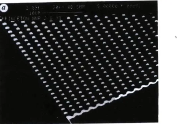
"The micrograph shows the 0.15 pm-high posts, diameter 1.0 pm, and center to center spacing of 2.0 pm". Adapted from Volkmuth et al. [2]. 24 1-3 "Structure of the microfabricated device incorporating the anisotropic

nanofilter array (ANA). Scanning electron microscopy images show details of different device regions (clockwise from top right: sample injection channels, sample collection channels and ANA). The inset shows a photograph of the thumbnail-sized device. The rectangular ANA is 5 mm x 5 mm. Shallow regions are 1 pm wide, 1 pm long, 55 nm deep and spaced by 1 pm x 1 pm square silicon pillars. Deep channels are 1 pim wide and 300 nrm deep. Injection channels connected to the sample reservoir (1 mm from the ANA top left corner) inject biomolecule samples as a 30-mm-wide stream." Adapted from Fu et al. (2007) [3]. . . . . 25 1-4 Molecules follow different trajectories based on their size. Adapted

from Fu et al. (2007) [3]. . . . . 26 1-5 Schematic of the nanofilter array. . . . . 26 1-6 Ogston entropic transition, adapted from Fu et al. (2006) [4] . . . . . 27 2-1 Root mean square end-to-end distance versus contour length using

3-1 DNA descretization into N - 1 links and N beads. . . . . 42 3-2 DNA molecule divided into N segments, N beads and N-1 connecting

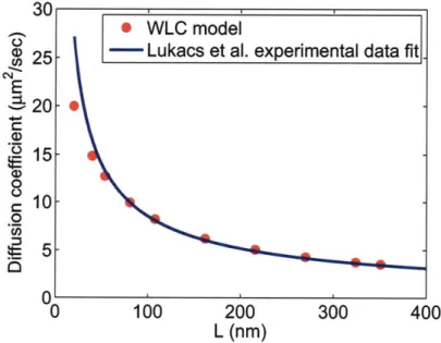
lin ks. . . . . 43 3-3 WLC beads positions. . . . . 44 3-4 Comparison between our simulation results and the experimental data

of Lukacs et al. [7] for the diffusion coefficient of dsDNA molecules in w ater. . . . . 50 3-5 SEM image and more realistic geometry. . . . . 53 3-6 WLC model simulation results for different geometries. . . . . 54 3-7 Probability density distribution for L = 108 nm, Ea, = 63.4 V/cm. 55 3-8 Probability density distribution for L = 216 nm, Eay = 63.4 V/cm. 56 3-9 Schematic of one period of the asymmetric nanofilter array. . . . . 57 3-10 Net velocity of dsDNA molecules of different lengths in asymmetric

device under AC fields of varied strength. . . . . 58 3-11 Probability density distribution in asymmetric channel with AC field

for L = 270 nm, Ea = 100 V/cm (Pet = 17.8). . . . . 59 4-1 Rigid rod-like model. . . . . 62 4-2 Comparison between WLC and rigid-rod model results (ideal geometry). 67 4-3 Comparison between WLC and rigid-rod model results (realistic

ge-om etry). . . . . 67 4-4 Torque effect on DNA mobility (ideal geometry). . . . . 68 5-1 Energy landscape of a charged DNA molecule along the nanofilter

chan-n el. . . . . 72 5-2 Comparison between the rigid-rod like model and the

partition-coefficient-based m odel. . . . . 76 5-3 Comparison between the experimental data and the

partition-coefficient-based m odel. . . . . 77 6-1 Variance reduction example adapted from Ottinger et al. [8]. . . . . . 81

6-2 One dimensional forced diffusion on non-interacting Brownian particles. 85 6-3 No flux boundary condition using deviational particle method. ... 87 6-4 Implementation of no flux boundary condition using deviational particles. 88 6-5 Comparing deviational particle results with analytical solution 6.17. . 89 6-6 Comparing variances of deviational particle method and regular

Brow-nian Dynamics as a function of translational P6clet number. . . . . . 90 6-7 Boundary effects and updating weights. . . . . 94 6-8 Comparing importance-weight method results with analytical solution. 95 6-9 Device regions. . . . . 96 6-10 Comparing importance-weight results and regular Brownian Dynamics

model for small translational Peclet number in the ideal experimental device. . . . . 98 6-11 Comparing variances of importance-weight method and regular

List of Tables

2.1 Summary of dimensional values of key physical parameters. . . . . 38 2.2 Summary of the dimensionless numbers. . . . . 38

Chapter 1

Introduction and background

1.1

Separation of biological molecules using

mi-cro/nanofluidic devices

Separation of biological molecules such as DNA and proteins is of great importance for the chemical and pharmaceutical industries [9, 10, 11]. For example, separation of DNA is used for crime investigation [12, 13 and detection and identification of biomarkers in urine [14], while separation of proteins is used for early detection, treatment and prevention of cardiovascular disease [15], and can be similarly applied to lung cancer studies [16].

In recent years, several researchers focused on fabricating regular nanopatterned sieving structures instead of using porous gel media to separate various types of biological molecules. Duong et al. [1] separated long DNA molecules using the one dimensional microfluidic device with a well defined patterned structure shown in Figure 1-1. Their polydimethylsiloxane (PDMS) microstructure allowed short A-DNA molecules to migrate faster than long T2-DNA. In another study, Volkmuth et al. [2] used microlithography to manufacture a two-dimensional nanostructured array to study the motion of long DNA molecules in a well defined topology as shown in Figure 1-2. Their experimental data shows that they were able to separate DNA molecules up to a length of ~ 100 kbp.

A /**""''''"'""t~ PoMs

i)

ii)-il) PDMS iv) PDMS

Microscope glass slide

Fig. 1. (A) Process diagram of microchannel fabrication. (i) Convert shaped microchannel mould is fabricated with SU-8. (ii) PDMS is poured and cured over the mould. (iii) PDMS is released from the mould. The microchannel is thus replicated into PDMS. (iv) Reservoirs are punched through PDMS. The microchannel is closed with microscope glass slide. (B) The drawing describes the variables of the periodical cavities (a-d) in the microchannels. The channel width d is used to define the channel layouts. (C) SEM top view of moulded 1.5 im and (D) 3 s~m PDMS microchannel.

Figure 1-1: Schematic diagrams and SEM images of the microchannel manufactured by Duong et al. [1]. Adapted from Duong et al. [1].

Figure 1-2: Volkmuth's figure shows an electron micrograph of a corner of an array. "The micrograph shows the 0.15 tm-high posts, diameter 1.0 pm, and center to center spacing of 2.0 pm". Adapted from Volkmuth et al. [2].

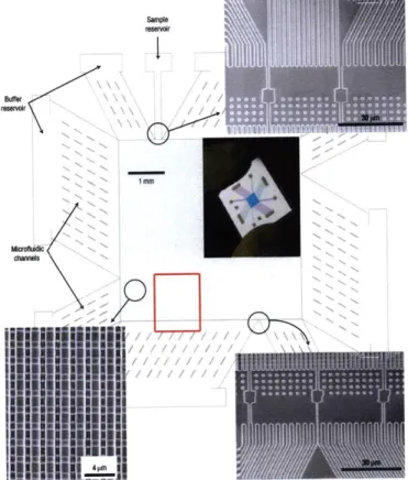
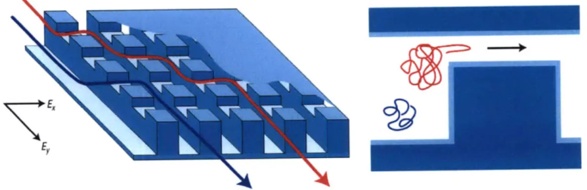
Fu et al. [3] developed a two-dimensional anisotropic nanofluidic array (see Figure 1-3 from Fu et al. (2007)) to separate short biological molecules. The main reason for this two-dimensional anisotropic sieving structure was to achieve continuous-flow separation. This feature is of great importance for biomarker detection and biosensing with microfluidic systems, since the continuous harvesting of biomolecules of interest would enhance the detection limit for the downstream analysis. The two-dimensional physical landscape of the device can be thought of as a large number of rows of nanofilters separated with deep channels. When biomolecules of different size are injected into the deep channel, they can occasionally jump to the next deep channel

through the passage of the nanofilter. The jumping passage rate depends on their size. Hence, molecules will follow different trajectories depending on their size as shown in Figure 1-4. reservoir wilcrokd"

~

IM

/-i//

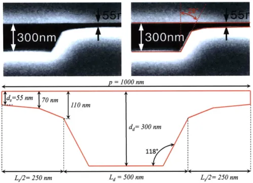
Figure 1-3: "Structure of the microfabricated device incorporating the anisotropic nanofilter array (ANA). Scanning electron microscopy images show details of different device regions (clockwise from top right: sample injection channels, sample collection channels and ANA). The inset shows a photograph of the thumbnail-sized device. The rectangular ANA is 5 mm x 5 mm. Shallow regions are 1 pm wide, 1 pm long, 55 nm deep and spaced by 1 pm x 1 pm square silicon pillars. Deep channels are 1 pm wide and 300 nm deep. Injection channels connected to the sample reservoir (1 mm from the ANA top left corner) inject biomolecule samples as a 30-mm-wide stream." Adapted from Fu et al. (2007) [3].

In this Thesis we focus on a specific one-dimenstional device design based on the work of Fu et al. [4] shown in Figure 1-5. This device consists of a large number (N, ~ 50, 000) of alternating shallow and deep regions etched in a silicon wafer. Biological molecules (DNA, protein) of contour length L, persistence length L, and radius of gyration Rg, driven by an electric field through this periodic array of constrictions are

>KE,

Figure 1-4: Molecules follow different trajectories based on their size. Adapted from

Fu et al. (2007) [3].

size-separated because their size-dependent mobilities result in size-dependent travel

times. Typical [4] dimensions for the shallow and deep region depths and period are

d, ~ 55 nm,

- 300 nm and p ; 1 pm, respectively.

d,

=55

nm

d=

300

nm

p=l

upm

Figure 1-5: Schematic of the nanofilter array.

1.2

Ogston sieving versus entropic trapping

Molecule mobility in these devices is not a monotonic function of molecule length.

As Figure 1-6 shows, molecule mobility initially decreases and then increases with

molecule length. This leads to two distinct separation regimes: Ogston sieving, where

short molecules travel faster than longer molecules and entropic trapping, in which

longer molecules travel faster than shorter molecules. Ogston sieving takes place when

the molecule radius of gyration is on the order of, or smaller than, the narrow region

depth (d,). In this case, entering the narrow region is a matter of reorientation: short molecules have a larger number of allowable conformations in which they can enter the shallow region in comparison to longer molecules; as a result they spend less time trying to enter the deep region and consequently travel faster in the device (i.e. they will have a higher mobility compared to longer molecules).

entropic trapping 6 5

CD

~45.31

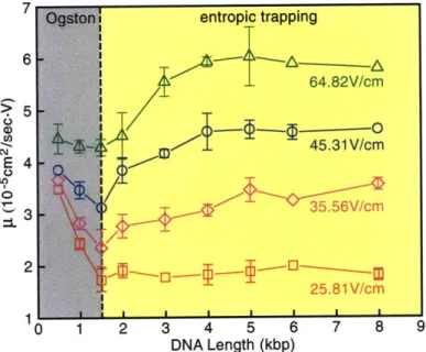
FIG. 3 (color online). Mobility y- as a function of DNA length. DNA fragments were extracted after agarose gel separation. The nanofilter array has d, = 73 nm, dd = 325 nm, p = 1 ym. The relative large statistical error bars (drawn if larger than the symbol) are likely due to the low DNA concentrations. The left and right shaded (gray and yellow online) areas indicate Ogston sieving and entropic trapping, respectively. The transi-tion points are marked with the vertical dashed line drawn for DNA length = 1.5 kbp.

Figure 1-6: Ogston entropic transition, adapted from Fu et al. (2006) [4].

Transition to the entropic trapping regime occurs when the molecule radius of gyration is larger than the shallow region depth. In the experimental results of Fu et al. [4] in Figure 1-6, the shallow region depth was d, = 73 nm. The transition occurs at a DNA length of 540 nm (1500 bp), which has a radius of gyration of - 80 nm, as expected.

-In the entropic trapping regime, due to their size, the molecules are not freely moving in the device but rather spend most of their time attempting to enter the deep region. While attempting to enter, longer molecules will have longer segments in contact with the shallow region (in the transverse (z) direction), and thus higher probability that some segment of the molecule will enter and pull the remaining part of the molecule. In other words, longer molecules have a higher probability of entering the shallow re-gion and hence have a faster travel velocity in the nanofilter (i.e. they have a higher mobility compared to shorter molecules) [17].

The focus of this Thesis is on Ogston-regime sieving. In particular, we are interested in the separation of short, L < 950 bp (340 nm), dsDNA molecules using nanofilter arrays [4, 18] as described previously in Section 1.1. The radius of gyration of the longest DNA molecule (340 nm) is 63 nm which is close to the shallow region depth

d, ~ 55 nm.

1.3

Modeling of biological molecule separation

In this Thesis, we focus on the development of a Brownian Dynamics (BD) simula-tion framework for modeling the performance of nanofluidic separasimula-tion devices. The ultimate goal of this research is the development of robust simulation methods which can replace costly experimental setups for device design and optimization.

Theoretical modeling of this process is very desirable for gaining fundamental understanding, device optimization and parameter exploration [19, 20, 21]. Despite their small sizes, these devices contain a very large number of solvent molecules making classical molecular dynamics simulations intractable. In other words, for an efficient model, some degree of coarse-graining is required. In this work we show that for the short molecules studied here, a Brownian Dynamics (BD) formulation strikes a good balance between fidelity-e.g. agreement with experimental data-and computational efficiency (compared to more expensive coarse-grained techniques such as Dissipative Particle Dynamics [22]). A more complete presentation of our rationale

for choosing the Brownian Dynamics method can be found in Section 2.2.

Although BD simulations of biological molecule separation have appeared in the literature before [20, 23], those studies have focused on molecules that are sufficiently longer than Lp, which put the separation mechanism in the entropic trapping regime

[4];

The objective of this Thesis is to construct sufficiently realistic and efficient models that can quantitatively describe experimental data that are relevant to current engi-neering practice (low-field). Our models will be guided/validated by the experimental data of Fu et al. [4].

1.4

Brownian Dynamics

Brownian Dynamics [24, 25, 26] is a method for coarse-graining a molecular descrip-tion of Brownian particles to the mesoscopic level [27). It corresponds to the sim-plified version of Langevin Dynamics [28] in the limit where acceleration effects are negligible (overdamped Langevin dynamics). BD formulations achieve considerable computational efficiency gains by treating "explicitly" only the particles of interest; the remaining particles are treated "implicitly" [29] by ignoring the details of their motion and only accounting for their collective effect on the explicit particles, namely, viscous resistance to the latter's motion and random "kicks" modeling the net effect of collisions of the latter with the implicit particles.

As can be expected, such formulations lend themselves naturally to modeling dilute systems of solute particles (e.g. macromolecules) in the presence of a solvent; by focusing only on the solute particles of interest and not solving the equations of motion of the large number of solvent particles, BD formulations enable calculations

that would have been out of reach of more traditional ab-initio methods. One of the disadvantages associated with this coarse-graining process is the loss of long-range particle-particle interactions [29]; hydrodynamic interactions may be included in the model [25] at the expense of some algorithmic complexity and computational cost. Using the Chebychev polynomial approximation [30] as originally suggested by Fixman [31], as well as novel schemes for truncating the range of electrostatic and hydrodynamic interactions [32], has resulted in efficient methods that have enabled the practical simulation of long-chain-molecule hydrodynamics in microdevices [33, 32].

1.5

Thesis outline

In Chapter 2, we present a brief discussion of the important dimensional and non-dimensional numbers relevant to the physics of the problem which will help us ana-lyzing the motion of the DNA molecules in the nanofilter. Based on this analysis, we discuss the different numerical approaches that one can choose to tackle the problem of interest.

In Chapter 3, we present the Worm-Like-Chain (WLC) BD model [34, 35, 36]. This model includes the effects of bending and stretching stiffness and provides the most accurate description for the DNA molecule. Our implementation of the Worm-Like-Chain model is in line with the work of Allison et al., Hagerman et al., Lewis et al, Klenin et al. [34, 35, 36, 37] and is thus different from Bead-Spring models that are usually used for long molecules [38, 39]. The resulting Brownian Dynamics for-mulation includes hydrodynamic interactions between beads, and closely models the experimental set up of Fu et al. [4], whose data are used for validation.

In Chapter 4, we present a simpler BD model which treats the DNA molecule as a rigid-rod [40]; this results in significantly reduced computational requirements com-pared to the WLC model of Chapter 3. On the other hand the model is limited to

short rigid rod-like DNA molecules of length L < LP.

In Chapter 5, we present a further simplified BD model which treats the DNA molecules as non-interacting point particles and accounts for their orientational de-grees of freedom through an entropic barrier. The point particle-coefficient-based model we present is based upon the work of [41]. This model is the most efficient and simplest to implement but again is limited to very short, essentially rigid (L < Lp) molecules. The simplicity of this model makes it ideal for applying variance reduction ideas for reducing the statistical uncertainty associated with its predictions.

In Chapter 6, we present a variance reduction methodology for the BD model of Chap-ter 5. This work extends the original ideas of Baker and Hadjiconstantinou [42, 43] and Al-Mohssen and Hadjiconstantinou [44, 45] who presented variance reduction techniques for solving the Boltzmann equation for low-speed gas flow. Specifically we develop variance reduced BD models based on both formulations used in the above work and show that the formulation of Al-Mohssen and Hadjiconstantinou is more suitable for the applications considered here.

Chapter 2

Computational model, dimensional

and non-dimensional analysis

2.1

Dimensional and non-dimensional analysis

In this section we review some characteristic physical magnitudes and develop relevant non-dimensional numbers that affect the separation process.

2.1.1

Dimensional analysis

1. Stokes drag on a bead

The drag coefficient on a bead of radius a is given by the Stokes formula

<bead

where r, is the viscosity of the solvent (water), which is taken to be 1.18 x

10- Pa - s following the recent experimental results of Hsieh et al.

[46]

Polymer relaxation time T, can be estimated using Rouse's [47, 48] model:

_ (beadL2

TrRouse _3r2

kBT

or using Zimm's model [48, 49]:

n

(=

(2.3)

Trzim _v/-7kBT

( where kB is the Boltzmann constant, T is the temperature and Lk = 2L,

108 nm is 1 Kuhn length for a dsDNA molecule. Using Equation 2.3 we find that the relaxation time for DNA molecules ranging between 20 - 340 nm ranges

from 9.6 x 10-6 to 6.5 x 10-4 seconds. 3. Brownian relaxation time

Brownian relaxation time is defined by the ratio of the Brownian molecule mass divided by the average drag on the molecule:

TB = Mass _ pDNA7rDNAL (2.4)

Drag

CZimm

where PDNA = 930 kg/r 3 [50] is the DNA density, rDNA ~ 1 nm is the DNA geometric radius and

CZimm

Zimm's model [49, 48] given by:

CZimm

8

The Brownian relaxation time ranges from 10-13 to 10-12 seconds for DNA of length 20 to 340 nm. The smallest timescale we are interested in simulating is on the order of:

. ~ ~ dS (Zimm(onm) 10-4 seconds (2.6)

D

the largest diffusion coefficient which corresponds to the smallest DNA molecule of interest (20 nm). We estimate the largest diffusion coefficient using the Zimm model [49] which agrees very well with the experimental measurements [51].

Since the smallest timescale we are interested in simulating is much larger than

TB, this means that our system is highly damped and we can neglect inertia in

our simulations.

4. Radius of gyration

The mean square radius of gyration of the Worm-Like-Chain Kratky-Porod model was first calculated by Benoit and Doty [52] and is given by:

(R9 )

LL - LP + 2-= - 2-

- exp

(2.7)

(J?2)

_ )

3 L _2.L7

For the experimental data of Fu et al. [4] the radius of gyration of the longest DNA molecule (270 nm) is 53.6 nm which is almost equal to the shallow re-gion depth. This places the separation process in the Ogston regime (where the primary sieving mechanism derives from the steric hindrance due to the re-striction) or the early transition region between the Ogston regime and entropic trapping [4].

5. Root mean square end-to-end distance

The mean square end-to-end distance of a flexible molecule as predicted by the Kratky-Porod model [5, 6] is given by:

(L e) = 2LL, 1 L- 1 - exp (2.8) In our study the dsDNA persistence length was about 54 nm. For a 54 nm DNA molecule, the Kratky-Porod model (Equation 2.8) predicts about 17% difference between the contour length and the root mean square end-to-end distance of the molecule (see Figure 2-1). In other words a rigid-rod-like model is expected to be a reasonable model for molecules up to 54 nm (150 bp) in length. Since in this Thesis we study molecules with length up to 340 nm

- Contour length (L)

50 - Root mean square end-to-end (L )1/2 17% 40 E30-20 10 1 Persistence length 0 0 10 20 30 40 50P 60 Contour length L (nm) P

Rigid-rod model

Worm-Like-Chain model

Figure 2-1: Root mean square end-to-end distance versus contour length using

Kratky-Porod model [5, 6].

(950 bp) a Worm-Like-Chain model, which takes DNA backbone flexibility into

account, is used.

2.1.2

Non-dimensional analysis

1. Translational Peclet number

The translational Peclet number Pet compares the importance of advection

relative to diffusion. In this nanofluidic device, the translational Peclet number

can be defined as

Pet = =EP _ q'LEavp (2.9)

D kBT

where y ~ 6.3 x 10- cm

/Vs is the free solution mobility, Ev is the applied

electric field, p ~ 1000 nm is the device pitch length which is the

character-istic distance over which advection and diffusion rates are compared, D is the

molecule diffusion coefficient and q' is the DNA effective charge per unit length

discussed in detail in section 3.7.1. In the experimental setup of Eu et al. [4] the minimum and maximum translational P6eclet numbers are as follows:

" Minimum translational Peclet number Pet,,

0.25

corresponds for the case where E, = 10 V/cm and LDNA = 18 nm

(short-est DNA molecule used in the experiments). Such molecule has a diffusion coefficient D1 nm ~25 1 pm2/

e Maximum translational Peclet number Pet,. ~ 11.5

corresponds for the case where E, = 64 V/cm and LDNA = 270 nm

(longest DNA molecule used in the experiments). Such molecule has a diffusion coefficient D270 nm ~ 3.5 pm2 s.

2. Rotational Peclet number

The relative effects of rotation due to the electric field gradient and rotational diffusion are quantified by the rotational Peclet number Per [19] given by:

Pe, =

(t

6

)

(2.10)

v + E 12kBT

where c = d,/dd is the ratio of the shallow region depth d, - 55 nm to the deep region depth dd ~ 300 nm, v is the length ratio between the shallow and deep region. The maximum rotational Peclet number - 0.04 corresponds to the longest DNA molecule (L = 108 nm) for which we assume a rigid-rod-like model

- see Chapter 4 for details - along with the highest electric field E, = 64 V/cm.

3. Reynolds number

Reynolds number measures the ratio of inertial forces to viscous forces. Reynolds number based on the molecule contour length ReLDNA is given by

ReLDNA - VDNAL ppELDNA (2.11)

where v, = qs/p = 1.18 x 10-6m2/s is the fluid (water in our case) kinematic viscosity, p is the free-solution mobility. The maximum Reynolds number in

the experimental setup is 10-5

2.1.3

Summary

We summarize all these dimensional and non-dimensional numbers in Table 2.1 and Table 2.2, respectively. Note that the minimum and maximum values do not neces-sarily correspond to the shortest and longest DNA molecule.

Table 2.1: Summary of dimensional values of key physical

Minimum

parameters.

Maximum Translational P6eclet number Pet 0.25

Rotational P~elet number Pe, 3.7 X 104

Reynolds number ReL 10-7

Table 2.2: Summary of the dimensionless numbers.

From these values we can draw the following conclusions which will be used throughout our modeling efforts:

1. The separation process falls into the Ogston sieving regime

2. Particle inertia can be neglected since we are in a highly damped system. 3. The translational diffusion and advection effects are both equally important

since the translational Peclet number is - 0(1).

4. The rotational diffusion is dominant in comparison to rotational torque due to electric field gradient since the rotational Peclet number is very small (Per <

DNA Length L 18 nm (50 bp) 340 nm (950 bp)

DNA relaxation time Tr 9.6 x 10-6 (s) 6.5 x 10-4 (s) Brownian relaxation time TB 10-13 (s) 10-12 (s)

Radius of gyration Rg - 63.1 (nm)

Root mean square end-to-end i 17.1 (rm) 175.8 (m) distance

0.05 < 1). This will help us develop a simple partition-coefficient-based model in Chapter 5.

5. Inertial forces are negligible compared to viscous forces and drag forces will be estimated using Stokes law [53].

2.2

Why Brownian Dynamics?

Efficient simulations of DNA separation are difficult to achieve due to the multi-scale and multi-physics nature of the problem. Specifically, although microscopic in nature, the device dimensions are sufficiently large, and the separation timescale sufficiently long (seconds), to make Molecular Dynamics (MD) [24] simulations intractable. On the other hand, a continuum approach, e.g. through computational fluid dynamics (CFD) [54], places insufficient emphasis on the dominant physics of interest. Specif-ically, a CFD approach focuses exclusively on a detailed hydrodynamic description while neglecting Brownian (entropic) effects. Although addition of Brownian fluctua-tions to continuum (Navier-Stokes) formulafluctua-tions has been investigated [55], previous work has been limited to simple systems and does not extend easily to the macro-molecules of interest here. Moreover, the computational complexity associated with CFD approaches including rigid (rod) or semi-rigid (Worm-Like-Chain) moving ob-jects in the computational domain makes these methods not preferable in view of the above limitations.

For the above reasons, mesoscopic approaches have attracted some interest. Dis-sipative Particle Dynamics (DPD) [56] has attracted interest due to its ability to nat-urally capture thermal fluctuations and the DNA particulate nature. DPD reduces computational cost (compared to MD) by coarse-graining length and timescales by "lumping" many actual molecules into computational particles that obey appropri-ately modified equations of motion. Unfortunappropri-ately, this technique is too computa-tionally expensive for our application since the coarse-graining is limited by the need to capture details at the level of the shallow region depth d, ~ 55 nm. In other words, the computational cost of DPD will be very close to that of MD for the systems of

interest to this Thesis. We also mention the Lattice Boltzmann method [57] which may be useful as a qualitative simulation tool.

Given the above considerations we have decided to use a Brownian Dynamics (BD) [38, 26, 40, 34, 25] approach. As explained in Section 1.4, in BD only the equations of motion of the molecules of interest (here, DNA) are solved, while the solvent is modeled as a continuum medium interacting with the molecule of interest through random (Brownian) and deterministic (drag) forces.

In this Thesis we explore BD models of varying degrees of coarse-graining in search of computational efficiency while retaining satisfactory agreement with the experimental data of Fu et al. [4]. Specifically, we present three Brownian Dynamics models:

1. Flexible Worm-Like-Chain (WLC) model discussed in detail in Chapter 3. 2. Rigid rod-like model discussed in detail in Chapter 4.

3. Point-particle partition-coefficient-based model discussed in detail in Chapter 5.

Chapter 3

Flexible Worm-Like-Chain (WLC)

model

3.1

Introduction

In this Chapter we focus on the development of a Brownian Dynamics [26, 38, 34] simulation framework for modeling the performance of the nanofluidic separation devices discussed in Chapter 1. This work utilizes the Worm-Like-Chain (WLC) model [34, 35, 36] which includes the effects of bending and stretching stiffness. Our implementation of the Worm-Like-Chain model is in line with the work of Allison et al., Hagerman et al., Lewis et al, Klenin et al. [34, 35, 36, 37] and is thus different from Bead-Spring models that are usually used for long molecules [38, 39].

The resulting Brownian Dynamics formulation includes hydrodynamic interac-tions between beads, and closely models the experimental set up of Fu et al. [4], whose data are used for validation. The material presented here has appeared in a more condensed form in [58].

3.2

The WLC model

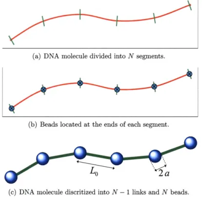
In typical WLC treatments [34], the molecule is modeled as an elastic chain consisting of N beads of radius a connected by N - 1 elastic links of average length Lo as shown

in Figure 3-1. In the present work we use a slightly modified discretization which

(a) DNA molecule divided into N segments.

(b) Beads located at the ends of each segment.

(c) DNA molecule discritized into N - 1 links and N beads. Figure 3-1: DNA descretization into N - 1 links and N beads.

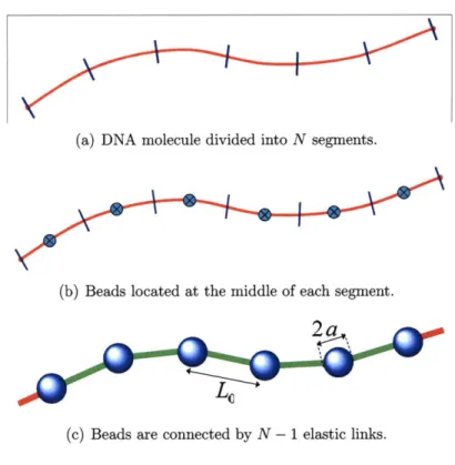
features N beads and N segments, as shown in Figure 3-2. In this discretization, each bead represents the same fraction of chain length and hence makes the application of a common bead size and effective charge more justified. The beads are connected by N - 1 elastic links (shown in green in Figure 3-2). The half segments on each end of the molecule are assumed to be an extension of their nearest link, and are used in defining the molecule shape, e.g. during boundary condition imposition. Our numerical formulation otherwise follows the work of Klenin et al. [34]; the chain elasticity includes stretching and bending contributions.

Our chain conformation is specified by the locations ri, i = 1,... , N of the N

beads comprising the chain and which are located at the vertices of the N -I straight links. The links are represented by the vectors si = ri+1 - ri, i = 1,... , N - 1; we define si =

Isi|

(a) DNA molecule divided into N segments.

(b) Beads located at the middle of each segment.

LC

(c) Beads are connected by N - 1 elastic links.

Figure 3-2: DNA molecule divided into N segments, N beads and N

-

1 connecting

links.

3.3

Equations of motion

The governing equations for the system of these N beads are Langevin-type equations

of motion:

j=N

m;ir =

-Z

(

+

+

1,...

N

j=1

where the change in momenta mji5 is balanced by the sum of all the external forces

applied on bead i. The drag force exerted by the surrounding fluid is accounted for by

-Zj=N

(igjj

while

systematic) is a systematic force due to the interaction between

the beads due to the stretching and bending forces between the beads as well as the

external electric field force. Finally, F

represents randomly fluctuating forces

exerted on each bead by the surrounding fluid. The systematic forces are discussed

in more detail below.

2a

/ -4

-. 1#

Figure 3-3: WLC beads positions.

3.3.1

Systematic forces

The systematic forces mentioned above can be divided into the stretching and bending

forces between beads, in addition to the external electric field force. In order to

calculate the stretching and bending forces we start by calculating their respective

stretching and bending energies.

3.3.1.1

Stretching force

Following Klenin et al.

[34],

we define the stretching energy for each segment i as

E stretchin Lo _ -si

kBT (LO6)2

(3.2)

kBT

_{2 ( LoS}

where kB is the Boltzmann constant, T is the temperature, LO is the link equilibrium

length and J is the stiffness parameter chosen such that

is approximately equal

to the variance of the link length distribution.

Hence the stretching force on the ith vertex from the (i + 1)th one is parallel to

the ith link and is given by:

Fstretching) - L)

isext (i -L)

(3.3) kBT

(Loo)

Finally, the total stretching force on the ith vertex is

F'stretchin") - -F(stretching) _i-1,next + F(stretching) _i,next (3.4)

3.3.1.2

Bending force

Similarly, we start by defining the bending energy for the ith joint as:

E(bending)

i

n2(3.5)

-

-a

kBT bendingi

35

where

#i

(L

(1

Here the dsDNA persistence length was taken to be L, = 54 nm [4, 59].

The bending force is calculated from the bending energy. The bending force acting on the ith vertex from the (i

+

F(bending) 2 CbendingIi

i,next 2a e bi _{x ei}

(3.7)

kBT Si

where

fpi

/

F(bending) _i,prev 2bnig3

p_

2_axending/3

i x ei-1 _(3.8)

kBT Si-1

Finally, the total bending force for the ith vertex is

3.3.1.3 Electric field force

The electric field force assigned to each bead is calculated using the following equation:

FI Electric) = qbeadE

I

where qbead is the effective charge on each bead. The latter is equal to the effective charge of the DNA molecule (see Section 3.7.1) divided by the total number of beads.

Elri is the value of the electric field at the position (ri) of the bead.

The electrostatic force is calculated based on the bead effective charge and the electric field due to the externally applied voltage difference across the device (AV). The electric field is pre-computed on a triangular grid with maximum edge size of approximately 2 nm assuming insulating boundary conditions at the walls using the MATLAB Partial Differential Equation Toolbox. An approximation to this solution is stored on a square grid for quick access; each square has a side of 5 nm. The piece-wise constant electric field value associated with every square is the average value over all triangle centroids within the square. Note that due to the extremely fine initial triangular grid (more than 10' elements) and the very fine square "interpolation" grid (more than 10000 squares) the error associated with this approximation is negligible compared to the modeling approximations and experimental uncertainties involved.

3.4

Numerical integration algorithm

The equation of motion [34, 25] of each bead is integrated using the two-step algorithm of Klenin et al. [34]. In the first step we calculate a "predicted" displacement using

r (t + At) = rj(t) + Dj(t) At + Ri , i = 1, ... IN (3.11)

j=1 kBT

where At is the time step and F,(t) denotes the force on bead

j;

inter-action tensor between beads i and

j,

The random displacements R, are defined by

(Ri) = 0 (3.12)

(Rt ® Rj) = 2DjjAt (3.13)

and can be calculated from a weighted sum of normal random deviates [34, 25]. Fol-lowing the recommendation of Klenin et al., the diffusion tensor is updated every 10 time steps thus reducing the number of times the expensive factorization needs to be performed.

Finally, the second integration step is

N

F'.(t + At) -- Fj(t)

ri(t + At) = r'(t + At) + Di (t) k T ' i = 1, ... , N (3.14)

j=1

where F'(t

+

+

3.5

Hydrodynamic interactions

Hydrodynamic interactions between the beads are accounted for using the Rotne-Prager tensor [60]:

D, = DoI if i=j

Di = Do aI+ 2 + 2 1- 3 2if rj > 2a, i j

Arij a + r r

(3.15)

Dij=

I

1

-

I

irr

f

<

j

where Do = kBT/67rla, q, is the solvent viscosity, r = rj - ri, ri = |ri|, I is the unity tensor, and r 9 r denotes the dyadic product.

The bead radius is chosen such that a reference DNA chain-a chain of contour length equal to one persistence length-has the desired diffusion coefficient. This is further discussed in Section 3.7.

3.6

Boundary conditions

Interactions with the walls are steric; in other words, if during a move, part of the molecule extends beyond one of the system boundaries, the move is rejected. In

such a case, the molecule is assigned its original position, and a new step is taken which is again checked for boundary crossing. We have considered both including and neglecting the time increment during rejected moves; the difference to our results is negligible due to the small time step used which results in a number of rejected steps that is less than 1% of the total number of steps. Several researchers [23, 19] have used similar boundary conditions. Reflecting boundary conditions, whereby a molecule (or parts of a molecule) is returned to the domain by taking the mirror image of the "offending" move, have also been used in some studies [21].

3.7

Simulation parameters

In accordance with the experiments of Fu et al. [4], we consider dsDNA molecules of lengths 18 nm < L < 324 nm in a Tris-Borate-EDTA 5 x buffer which diminishes the effect of electro-osmotic flow [61). We consider average electric fields E, = AV/(pN,)

in the range 20 - 400 V/cm. The viscosity of the solvent (water) is taken to be 1.18 x 10-3 Pa - s following the recent experimental results of Hsieh et al. [46] for the buffer considered here.

The timestep was 10-1 s. This value was chosen such that all guidelines set by Klenin et al. [34] are satisfied. The total simulated time modeling the experiments of Fu et al. varied between 15 and 60 minutes (depending on the molecule length and electric field), and was such that the molecule traverses at least 10, 000 periods. We have also verified that the initial position and configuration of the DNA molecule does not affect our results. In fact, to make sure that no "initial condition" effects are present, we start collecting data on the distance traveled by the molecule after 108 timesteps of relaxation (no field) and 10' timesteps of motion under the action of the electric field. The statistical uncertainty in the majority of our calculations is less than 1%, leading to error bars that are smaller than the symbols on the graph. Error bars are given when the statistical uncertainty is sufficiently large for the error bars to be visible.

Although it would have been desirable to use the same discretization (e.g. same discretization length Lo) for all molecules studied here, the range of lengths stud-ied makes this impractical. In the interest of computational efficiency, the degree of coarse-graining increases in three steps: for 20.25 nm < L < 54 nm we use Lo = 6.75 nm; for 54 nm < L < 108 nm we use Lo = 13.5 nm; for 108 nm < L < 324 nm we use Lo = 27 nm. Our simulation method becomes inefficient for significantly longer molecules, primarily due to the hydrodynamic interactions.