Growth and bubbles: Investing in human capital versus having children

HAL Id: hal-02111823

https://hal-amu.archives-ouvertes.fr/hal-02111823

Submitted on 29 Apr 2019

HAL is a multi-disciplinary open access

archive for the deposit and dissemination of

sci-entific research documents, whether they are

pub-lished or not. The documents may come from

teaching and research institutions in France or

abroad, or from public or private research centers.

L’archive ouverte pluridisciplinaire HAL, est

destinée au dépôt et à la diffusion de documents

scientifiques de niveau recherche, publiés ou non,

émanant des établissements d’enseignement et de

recherche français ou étrangers, des laboratoires

publics ou privés.

Growth and bubbles: Investing in human capital versus

having children

Xavier Raurich, Thomas Seegmuller

To cite this version:

Xavier Raurich, Thomas Seegmuller.

Growth and bubbles:

Investing in human capital

ver-sus having children.

Journal of Mathematical Economics, Elsevier, 2019, 82, pp.150-159.

Growth

and bubbles: Investing in human capital versus having children

✩

Xavier

Raurich

a

_,

_{Thomas Seegmuller}

b,∗

a _{Departament d’Economia and CREB, Universitat de Barcelona, Spain}

b _{Aix-Marseille Univ., CNRS, EHESS, Centrale Marseille, AMSE, 5 Boulevard Maurice Bourdet CS 50498 F-13205 Marseille cedex 1, France}

Keywords:

Bubble; Sustained growth; Fertility; Human capital

a b s t r a c t

As it is documented, households’ investment in their own education (human capital) is negatively related to the number

of children individuals will have and requires some loans to be financed. We show that this contributes to explain

episodes of bubbles associated to higher growth rates. This conclusion is obtained in an overlapping generations model

where agents choose to invest in their own education and decide their number of children. A bubble is a liquid asset that

can be used to finance either education or the cost of rearing children. The time cost of rearing children plays a key role in

the analysis. If the time cost per child is sufficiently high, households have only a small number of children. Then, the bubble

has a crowding-in effect because it is used to provide loans to finance investments in education. On the contrary, if the time

cost per child is low enough, households have a large number of children. Then, the bubble is mainly used to finance the

total cost of rearing children and has a crowding-out effect on investment. Therefore, the new mechanism we highlight shows

that a bubble enhances growth if the economy is characterized by a high rearing time cost per child.

1. Introduction

Caballero et al.(2006) andMartin and Ventura(2012) show that episodes of bubbles are associated with larger growth rates. This empirical fact contradicts the results obtained in seminal contributions, where the existence of a bubble has a crowding-out effect on capital accumulation (seeTirole(1985) with exoge-nous growth orGrossman and Yanagawa(1993) with endogenous growth). Many recent papers have tried to conciliate the theory with the empirics, by providing some relevant explanations on the growth enhancing role of a bubble. Some of the underly-ing mechanisms are based on the existence of heterogeneous productive investments and bubble shocks (Martin and Ventura,

2012), the existence of financial constraints (Fahri and Tirole,

2012;Hirano and Yanagawa,2017;Kocherlakota,2009;Miao and

✩ _{This work has been carried out thanks to the financial support of the French}

National Research Agency, France (ANR-15-CE33-0001-01), the ECO2015-66701-R grant funded by the Government of Spain and the SGECO2015-66701-R2014-493 grant funded by the Generalitat of Catalonia, Spain. We would like to thank an anonymous referee for his comments and suggestions which really improve the paper. We also thank participants to the 21st T2M conference, Lisbon March 2017, the 2017 Asian Meeting of the Econometric Society, Hong Kong June 2017, the 16th Journées LAGV, Aix-en-Provence June 2017, The 17th SAET conference, Faro June 2017, the ASSET 2017 conference, Algiers October 2017, for their helpful comments.

Wang, 2018), the difference between liquid and illiquid assets (Raurich and Seegmuller,2015,2017), the existence of a bubble on a productive asset (Olivier,2000), among others.

In this paper, we provide a new mechanism explaining that bubbles are associated to episodes of higher growth. It is based on the trade-off faced by households between investing in education (human capital) and having children. The bubble is interpreted as the liquid asset used either for loans or for saving and that modifies this trade-off. Two pieces of evidence provide support to our mechanism relating investment in education with bubbles. First, there is a trade-off between investing in education and having children. As it is highlighted byMartinez et al.(2012),1 women and men with a higher level of education have fewer children. For instance, in US during the period 2006–2010, the average number of children ever born or fathered for women aged 22–44 years is 2.5 when the woman has no high school diploma or equivalent, is 1.8 when she has a high school diploma or equivalent, is 1.5 when she was in some college, and is only 1.1 when she has a Bachelor’s degree or a higher diploma. We observe the same trend for men. Similar findings can be found in

Jones and Tertilt(2008) orPreston and Hartnett(2011). This ev-idence clearly indicates that there exists a negative link between investment in education done at the beginning of the active life and the number of children the household will have later.

Second, any investment in education at the beginning of the active life requires some loans to finance it. This may be illus-trated by the case of student loans in the US. These loans have drastically increased since the beginning of 2000s, to become larger than $1 trillion in 2013 (Avery and Turner,2012;Dynarski,

2014). This amount is far from being negligible in comparison to other types of consumer loans, like auto loan or credit card.2

The previous evidence suggests that loans may facilitate in-vestment in education, modify fertility and, finally, affect the economic growth rate. In this paper, we consider that the support of the loan is a liquid asset without fundamental value, i.e. it is a bubble when it is positively valued. As mentioned, this asset can be used to finance investment in education, like fees for instance, which will enhance growth. However, it can also be a mean to save and transfer purchasing power to finance rearing costs of having children and consumption at the retired age. In this case, the introduction of this asset may increase population and reduce economic growth.

The purpose of this paper is to analyze the effect of the bubble on growth, through its effects on human capital and fertility. To this end, we develop an overlapping generations model with three-period lived agents. A household invests in education when young and chooses the number of children when adult, facing a time cost of rearing children. She is working when young and adult, while she is engaged in home production when old. In addition, each household trades the liquid asset when young and adult to take out loans or transfer purchasing power to finance some expenses, like the rearing costs. Finally, firms produce the final good using human capital and a linear technology that makes sustained growth possible.

Our main concern is to investigate when the existence of a bubble promotes growth. In such a case, we say that the bubble is productive. We show that this happens when the time cost of rearing a child is high enough. Indeed, when the time cost per child is low, the number of children is large and the total cost of rearing children is also high. As a consequence, the bubble is used to transfer wealth from young to middle-age, implying less investment in education. The bubble has a crowding-out effect on human capital and it reduces growth. On the contrary, when the time cost of rearing a child is high, the number of children is small and the total cost of rearing children is also small. As a consequence, the bubble is used to transfer resources from adult to young households. In this case, young agents take out some loans being short-sellers of the bubble, to increase their invest-ment in education. The bubble has a crowding-in effect on human capital, which means that it is productive. Finally, we show that the bubble can be productive even if the young households are not short-sellers of the bubble. This situation happens when the time cost of rearing a child takes intermediate values.

Our model also allows us to contribute to the debate on the link between population size and the asset price (Abel, 2001;

Geanakoplos et al.,2004;Poterba,2005). The main effect of pop-ulation on asset valuation discussed in this literature is based on the number of savers with respect to dissavers. A relative larger number of savers raises the demand of asset and, therefore, its price. We associate the asset price to the bubble on the liquid asset and a larger ratio of adult over young households means that the number of buyers of this asset is larger. We observe the same link found byGeanakoplos et al.(2004) between the asset price and the demography, i.e. a positive relationship between the value of the asset and the ratio of adult over young households.

This paper is organized as follows. In the next section, we present the model. In Section3, we analyze the economy without

2 _{Since 2007, annual borrowing from US students is larger than $100 billions}

(seeCol(2016), Figure 5).

bubble. In Section4, we characterize an equilibrium with a bub-ble. In Section5, we show the existence of an asymptotic bubbly balanced growth path (BGP). We analyze whether a bubble may be productive in Section6. In Section7, we interpret our results according to the crowding-out versus crowding-in effects. Con-cluding remarks are provided in Section8, while some technical details are relegated to an Appendix.

2. Model

Time is discrete (t

=

0

,

1

, . . . , +∞

) and there are two types of agents, households and firms.

2.1. Firms

Aggregate output is produced by a continuum of firms, of unit size, using labor, Lt, and human capital, Ht, as inputs. In addition,

production benefits from an externality that summarizes a learn-ing by dolearn-ing process and allows to have sustained growth. Fol-lowingFrankel(1962) orLjungqvist and Sargent(2004), chapter 14), this externality depends on the average human capital–labor ratio.

Letting ht

≡

Ht

/

Lt, ht represents the average ratio of

hu-man capital over labor. Firms produce the final good using the following technology:

Yt

=

F (Ht

, ¯

htLt)

The technology F (Ht

, ¯

htLt) has the usual neoclassical properties,

i.e. is a strictly increasing and concave production function sat-isfying the Inada conditions, and is homogeneous of degree one with respect to its two arguments.

Profit maximization under perfect competition implies that the wage

w

t and the return of human capital qtare given by3

w

t

=

F2(Ht

, ¯

htLt)h

¯

t (1)

qt

=

F1(Ht

, ¯

htLt) (2)

Note that while

w

t is the basic wage, i.e. the return from one

additional unit of labor, qt is the return from an additional unit

of human capital and, hence, it measures the skill premium.

2.2. Households

We consider an overlapping generations economy populated by agents living for three periods. An agent is young in the first period of life, adult in the second period and old in the third period. As it is argued by Geanakoplos et al.(2004), such a demographic structure is a reasonable representation of the households’ life-cycle.

Each household obtains utility from consumption at each pe-riod of time and from the number of children when she is an adult. Preferences of an individual born in period t are repre-sented by the following utility function:

ln c1,t

+

β

ln c2,t+1

+

β

2ln(c3,t+2

+

ϵ

)

+

µ

ln nt+1 (3) where

β ∈ (

0

,

1

)

is the subjective discount factor,

µ ∈ (

0

,

1

)

measures the love for children and nt+1is the number of children an adult has.4At each age, the household can consume the market good produced by firms. Hence, cj,t amounts for consumption of

3 _{We denote by F}

i(., .) the derivative with respect to the ith argument of the function.

4 _{The assumptionβ ∈(0,1) is not required for our results, but is quite}

natural when one interpretsβ as a discount factor. The assumptionµ ∈(0,1) means that love for children is less significant than the weight for consumption at the first period of life. It simplifies some proofs. Otherwise, some additional bounds onµshould be introduced.

this good when young (j

=

1), adult (j

=

2) and old (j

=

3). We also assume that when old, the household has a consumption of a home-produced good

ϵ >

0 which is, to simplify, a perfect substitute of the market good.5As explained byAguiar and Hurst

(2005), Hurst(2008) andSchwerdt (2005), home production at the retirement age is quite a realistic feature since it seems to solve the consumption puzzle when households are retired.6As in Kongsamut et al.(2001), we assume that the level of home produced good

ϵ >

0 is constant. An implication of this assump-tion is that the ratio between home producassump-tion and GDP declines. This result is consistent with empirical findings that establish that the productivity growth of home production is lower than the productivity growth of market production and home production over GDP or home production over market consumption strongly decreases in the US between 1970 and 2005 (Duernecker and Herrendorf,2015; McDaniel,2011). Note also that this assump-tion implies that home producassump-tion is independent of individual skills, which is consistent with empirical findings (seeDuernecker and Herrendorf(2015)).

While each household uses her time endowment for home production when old, she supplies labor to firms when young and adult. When young, this labor supply is one unit. In contrast, labor supply is endogenous when adult, as it depends on the number of children. We denote by 0

< ψ <

1 the fraction of time an adult spends for each child and, hence, the labor supply when adult is 1

−

ψ

nt+1. This specification is often used in the literature on fertility (de la Croix and Doepke,2003;Galor,2005).

When young, the household invests an amount et+1in educa-tion. This investment accounts for any cost of education, such as fees. Each unit invested in education will increase human capital at the next period. Therefore, it provides some additional returns

qt+1et+1at the period where the agent is working for the market good sector, i.e. when she is adult, but no return when she is retired, i.e. when old. While the basic wage is the only income when young, the income in the middle age also depends on the return of education.7

We introduce loans by assuming that households may also invest in a liquid asset without fundamental value when young (b1,t) and adult (b2,t+1). bi,t represents the value of the share of

this asset bought (bi,t

>

0) or sold (bi,t

<

0) by a young or an

adult household. There is a bubble on loans if this asset has a strictly positive price. Since this asset is supplied in one unit, the price

ˆ

Bt is given by the sum of the values of the shares held by

households living at the same time,

ˆ

Bt

=

Ntb1,t

+

Nt−1b2,t. When

ˆ

Bt

=

0 and b1,t

=

b2,t

=

0, the price of the asset is zero and there

is no bubble.

Accordingly, the budget constraints when young, middle age and old faced by a household born in period t are, respectively,

c1,t

+

et+1

+

b1,t

=

w

t (4)

c2,t+1

+

b2,t+1

=

qt+1et+1

+

Rt+1b1,t

+

w

t+1(1

−

ψ

nt+1) (5)

c3,t+2

=

Rt+2b2,t+1 (6)

where 0

<

nt+1

<

1

/ψ

. Population size of the generation born at period t is Nt. Therefore, the evolution of the population size of

the successive generations is given by Nt+1

=

nt+1Nt.

At this point, it is important to clarify that a bubble is a financial instrument that facilities consumption smoothing even

5 _{For home-produced good, the reader can refer to Gronau(1986) for a}

survey andBenhabib et al.(1991) for a macro-model with home production.

6 _{This puzzle is based on the observation that consumption expenditures are}

lower when individuals are retired, but the amount of consumption of goods is not lower.

7 _{Note that education and human capital have been introduced in a quite}

similar way in several papers. See for instancede la Croix and Michel(2007) or

Gente et al.(2015).

more than a traditional loan. In the following sections, we ana-lyze how this financial development affects the investment and fertility decisions of individuals. However, we already note that without home-produced good, i.e.

ϵ =

0, we could not define an equilibrium without bubble because the budget constraint(6)

would imply c3,t+2

=

0, which is not compatible with the utility function(3)with

ϵ =

0.

2.3. Equilibrium

At a symmetric equilibrium, ht

=

ht. Let us define

α ≡

F1(1

,

1)

/

F (1

,

1)

∈

(0

,

1) the capital share in total production and A

≡

F (1

,

1)

>

0. Using(1)and(2), we deduce that

w

t

=

(1

−

α

)Aht (7)

qt

=

α

A (8)

Equilibrium in the labor market requires that

Lt

=

Nt

+

Nt−1(1

−

ψ

nt)

=

Nt(1

−

ψ

)

+

Nt−1 (9) Investment in education done by young households directly becomes human capital in the next period: Ht+1

=

Ntet+1.8Using

(9), we get

et+1

=

ρ

(nt+1)ht+1 (10)

with

ρ

(nt+1)

≡

1

+

(1

−

ψ

)nt+1 (11)

3. The economy without bubble

We first analyze the economy without bubble, i.e. b1,t

=

b2,t

=

0. It corresponds to our benchmark case and it will allow us to compare the properties of equilibria with and without bubble.

3.1. Household’s choices

Maximizing utility (3) under the budget constraints (4)–(6)

with b1,t

=

b2,t+1

=

0, we obtain the level of productive investment and the number of children:

et+1

=

1 1

+

µ + β

[

(

µ + β

)

w

t

−

w

t+1 qt+1

]

(12) nt+1

=

µ

1

+

µ + β

w

t

+

w

t+1

/

qt+1

ψw

t+1

/

qt+1 (13) Investment in education is used by the households to smooth consumption between young and adult ages. Hence, the return from investment in education, qt+1, provides the measure of the discount rate in this economy without bubbles. This explains that, on the one hand, investment in education increases with the wage earned when young and decreases with the present value of the wage received when adult. On the other hand, the number of children increases with the lifetime income,

w

t

+

w

t+1

/

qt+1, but decreases with the discounted value of the rearing cost of having children

ψw

t+1

/

qt+1. As a result, the number of chil-dren decreases following an increase of the wage growth factor

w

t+1

/w

t.

8 _{Since human capital fully depreciates in one period, H}

t+1does not depend on Ht.

3.2. Bubbleless BGP

Let us denote by

γ

t+1

≡

ht+1

/

ht the growth factor of human

capital per unit of labor. Using(7),(8)and(13), we have

nt+1

=

µ

ψ

(1

+

µ + β

)

(

1

+

α

A

γ

t+1

)

(14) Since the wage increases with human capital per unit of labor and the number of children decreases with the wage growth factor, population growth reduces with the growth factor

γ

t+1. As it is illustrated byGalor(2005), this negative relationship is in accordance with what we observe in Western Europe and in US, Australia, New Zealand and Canada since one century.

Using(7),(8)and(12), we get

et+1

=

1 1

+

µ + β

[

(

µ + β

)(1

−

α

)Aht

−

1

−

α

α

ht+1

]

(15) Substituting(10),(11)and(14)in(15), we obtain

γ

t+1

=

α

A

ψ[µ + β

(1

−

α

)

] −

αµ

ψ

(1

+

αβ

)

+

αµ

≡

γ

wb (16)

where

γ

_wb

>

0 if and only if

ψ > αµ/[µ + β

(1

−

α

)

] ≡

ψ

0wb.

Substituting (16) in (14), we finally obtain the population growth factor:

n_wb

=

µ

ψ[µ + β

(1

−

α

)

] −

αµ

(17)

Note that n_wb

<

1

/ψ

if and only if

ψ > ψ

nwb, which is larger

than

ψ

0wband smaller than 1 if

µ < µ

nwb, with

ψ

nwb

≡

αµ

β

(1

−

α

)and

µ

nwb

≡

β

(1

−

α

)

α

(18)

We deduce the following proposition:

Proposition 1. Assume that 1

> ψ > ψ

nwb and

µ < µ

nwb

hold. Then, it follows that n_wb

<

1

/ψ

is satisfied and there exists

an equilibrium along which b1,t

=

b2,t

=

0,

γ

t+1

=

γ

wb and

nt+1

=

nwbhold for all t.

Without bubble, there is no transitional dynamics. We also note that there is sustained growth,

γ

_wb

>

1, if the productivity

A is high enough.

4. Equilibrium with a bubble

When there is a bubble (b1,t

̸=

0 and/or b2,t

̸=

0), a household

maximizes her utility (3) under the budget constraints (4)–(6)

taking into account that she can smooth consumption between the three periods of life using the liquid asset and between young and adult using investment in education. As a consequence, by arbitrage, we get Rt+1

=

qt+1. Then, the number of children and the consumptions over the life-cycle are given by

nt+1

=

µ

1

+

β + β

2

₊

µ

w

t

+

wt +1 Rt+1

+

ϵ Rt+1Rt+2

ψ

wt+1 Rt+1 (19) c1t

=

1 1

+

β + β

2

₊

_µ

(

w

t

+

w

t+1 Rt+1

+

ϵ

Rt+1Rt+2

)

(20) c2t+1

=

β

Rt+1 1

+

β + β

2

₊

_µ

(

w

t

+

w

t +1 Rt+1

+

ϵ

Rt+1Rt+2

)

(21) c3t+2

=

β

2_R t+1Rt+2 1

+

β + β

2

₊

µ

(

w

t

+

w

t+1 Rt+1

)

−

1

+

β + µ

1

+

β + β

2

₊

µ

ϵ

(22) Since when old, the market good produced by the firms is substitutable to a home-produced good, we should take care that

c3t+2is non-negative. However, as we will see later, the growing disposable income

w

t

+

w

t+1

/

Rt+1ensures a positive consumption c3t+2

>

0 at the long run equilibrium with sustained growth we are interested in.

Using(4),(6),(10),(20)and(22), we deduce that

b1t

=

β + β

2

₊

_µ

1

+

β + β

2

₊

_µ

w

t

−

1 1

+

β + β

2

₊

_µ

(

w

t+1 Rt+1

+

ϵ

Rt+1Rt+2

)

−

ρ

(nt+1)ht+1 (23) b2t+1

=

β

2_R t+1 1

+

β + β

2

₊

µ

(

w

t

+

w

t+1 Rt+1

)

−

ϵ

Rt+2 1

+

β + µ

1

+

β + β

2

₊

µ

(24) Because of the budget constraint (4), we observe that the share of the bubble bought by a young household decreases with investment in education and consumption at the first pe-riod of life. The first relation explains the negative effect of

ρ

(nt+1)ht+1on bubble holding when young (see(23)), while the second one implies that b1t decreases with the future wage, because consumption when young linearly rises with the life-cycle wage income (see Eq.(20)). By inspection of Eq.(24), we deduce that since the share of the bubble held in middle-age is the saving when adult, it increases with the disposable income

w

t

+

w

t+1

/

Rt+1. Because the wage linearly increases with human capital over labor, it explains that b2t+1will increase with ht+1, but at a lower rate. Finally, using Eq.(19), the number of children rises with the life-cycle wage income, but decreases with the dis-counted value of the rearing cost

ψw

t+1

/

Rt+1. Therefore, a higher wage when adult negatively affects the number of children.

These relations will allow us to deduce that b1t

/

ht, b2t

/

ht

and nt+1 are decreasing with the growth factor

γ

t+1. As we explained in the economy without bubble, the negative relation-ship between the number of children and the growth factor is observed in many developed countries since the beginning of the last century (Galor,2005). To properly derive these negative relationships, let us note

λ

t

≡

ϵ/

ht. Then, using(7),(8),(23)and (24)we determine the shares of the bubble held by the young and adult households detrended by human capital per unit of labor:

b1t ht

=

(1

−

α

)A

β + β

2

₊

_µ

1

+

β + β

2

₊

µ

(25)

−

γ

_t+1

[

ρ

(

γ

t+1

, λ

t+1)

+

1 1

+

β + β

2

₊

µ

(

1

−

α

α

+

λ

t+1 (

α

A)2

)]

≡

˜

b1(

γ

t+1

, λ

t+1) b2t ht

=

β

2₍₁

₋

_α

_)A 1

+

β + β

2

₊

_µ

(

α

A

γ

t

+

1

)

−

λ

t

α

A 1

+

β + µ

1

+

β + β

2

₊

_µ

≡

˜

b2(

γ

t

, λ

t) (26)

with

ρ

(

γ

t+1

, λ

t+1)

≡

ρ

(n(

γ

t+1

, λ

t+1)) and, using(19), we obtain n(

γ

t+1

, λ

t+1)

≡

µ/ψ

1

+

β + β

2

₊

µ

(

α

A

γ

t+1

+

1

+

λ

t+1

α

(1

−

α

)A2

)

=

nt+1 (27)

Equilibrium in the asset market means that

Nt+1b1t+1

+

Ntb2t+1

=

Rt+1(Ntb1t

+

Nt−1b2t) (28) where we recall that the value of the bubble at time t is given by

ˆ

Bt

=

Ntb1t

+

Nt−1b2t. Let Bt

≡

ˆ

Bt

/(

htNt−1

)

. Using Rt+1

=

qt+1,(8),

(25)–(27), the evolution of the population size and the definition of

λ

t, an intertemporal equilibrium is defined by

Bt

=

n(

γ

t

, λ

t)

˜

b1(

γ

t+1

, λ

t+1)

+˜

b2(

γ

t

, λ

t) (29)

Bt+1

=

α

A n(

γ

t

, λ

t)

γ

t+1

λ

t+1

=

1

γ

t+1

λ

t (31)

This system drives the dynamics of (

γ

t

,

Bt

, λ

t)

∈

R3++ for

all t and allows us to study the long run equilibrium. To study the transitional dynamics, it is important to note that Bt, which

represents the price of the liquid asset detrended by the ratio of human capital per unit of labor times the population size, is determined by expectations about the future and there is a bubble if and only if Bt

>

0. Therefore, this variable is not

predetermined. The growth factor

γ

tis also a non-predetermined

variable, because it is a function of human capital per unit of labor ht(

=

γ

tht−1)

=

Ht

/

Lt and Lt

=

Nt(1

−

ψ

)

+

Nt−1 is not predetermined as it depends on the endogenous number of children nt

=

Nt

/

Nt−1 chosen at period t. On the contrary, because ht implies that

γ

t is not predetermined,

λ

t

=

ϵ/

ht is

predetermined.

5. Asymptotic bubbly BGP

We focus on equilibria with a bubble growing at the same rate than human capital, i.e. with a positive and constant value of B, and sustained growth. This means that we are concerned with equilibria such that

γ

t

>

1, which implies that htwill tend to

+∞

in the long run. Along such a dynamic path,

λ

t

=

ϵ/

ht decreases

and tends to 0 when time tends to

+∞

. The dynamic system

(29)–(31)admits no steady state, but may converge asymptot-ically to a long run equilibrium with

γ

∗

_>

1 and

λ

∗

₌

0. This equilibrium will correspond to an asymptotic BGP with a positive bubble and sustained growth. Using Eqs.(29)–(31), it is a stationary solution (

γ

∗

_,

B∗

_{, λ}

∗ ) satisfying

γ

∗

_>

1,

λ

∗

₌

0 and

γ

∗ n(

γ

∗

,

0)

=

α

A (32) B∗

=

n(

γ

∗

,

0)

˜

b1(

γ

∗

,

0)

+˜

b2(

γ

∗

,

0)

>

0 (33)

Using Eqs.(27)and(32), the growth factor

γ

∗

is given by

γ

∗

=

α

A

ψ

(1

+

β + β

2

₊

_µ

₎

₋

_µ

µ

(34)

The inequality

ψ > µ/

(1

+

β + β

2

+

µ

) ensures that

γ

∗

_>

0. Then, there is sustained growth (

γ

∗

_>

1) if and only if

A

>

µ

α[ψ

(1

+

β + β

2

₊

µ

₎

₋

µ]

≡

A1 (35)

Using(25),(26),(32)and(34), the population growth factor is given by n(

γ

∗

,

0)

=

α

A

γ

∗

=

µ

ψ

(1

+

β + β

2

₊

_µ

₎

₋

_µ

≡

n ∗ (36) and the shares of the bubble bought when young and adult by

˜

b1(

γ

∗

,

0)

=

(1

−

α

)A

−

ψ

µ

A

[

1

+

α

(

β + β

2)

] ≡

˜

b ∗ 1 (37)

˜

b2(

γ

∗

,

0)

=

ψβ

2₍₁

₋

_α

_)A

ψ

(1

+

β + β

2

₊

µ

₎

₋

µ

≡

˜

b ∗ 2 (38)

We deduce that the detrended value of the bubble is

B∗

=

n∗

˜

b ∗ 1

+˜

b ∗ 2

=

A

[

1

+

αβ +

(2

α −

1)

β

2

]

ψ

(1

+

β + β

2

₊

_µ

₎

₋

_µ

(

ψ

b

−

ψ

) (39) with

ψ

b

≡

µ

1

−

α

1

+

αβ +

(2

α −

1)

β

2 (40)

In the following proposition, we summarize the existence of the asymptotic bubbly BGP and analyze also its stability. To that extent, note that from a mathematical point of view, the asymptotic steady state is a steady state of the dynamic system

(29)–(31). Therefore, we study its stability using a usual lineariza-tion, which allows us to deduce the stability properties in the neighborhood of the asymptotic BGP. Accordingly, we follow the method used inAcemoglu and Guerrieri(2008), Alonso-Carrera and Raurich(2015,2018) orSteger(2000), among others.

Proposition 2. Let

ψ ≡

µ

1

+

β + β

2 (41)

Assume that

α <

β+2β2

1+2β+3β2, A

>

A1and

ψ < ψ <

min

{

ψ

b

;

1

}

hold.

There is a unique asymptotic BGP with sustained growth (

γ

∗

_>

1,

n∗

_<

1

/ψ

) and a positive bubble (B∗

_>

0). In addition, the

equilibrium converges to this BGP.

Proof. SeeAppendix A. ■

This proposition establishes the existence of a unique asymp-totic BGP with a positive bubble and sustained growth. The economy converges to this asymptotic BGP, which is locally indeterminate. In the proof ofProposition 2, we show that there are two stable eigenvalues. Since one of these eigenvalues equals zero, in period one, there is a jump into a one-dimensional stable submanifold. The equilibrium exhibits local indeterminacy, because there is a unique state variable and the stable manifold is two-dimensional at t

=

0.9

Sustained growth requires both a sufficiently high productivity

A and a high enough

ψ

(see Eq.(34)). Indeed, a high time cost per child

ψ

reduces the incentive to have children. This implies that only a small amount of adult time is devoted to the total time cost of rearing children

ψ

n∗

(see Eq.(36)) and a large part of household resources can be used to invest in education, which promotes human capital and growth.

As we have seen previously, the shares of the bubble held by both young and middle-age households, and the number of children decrease with the growth factor. This implies that a positive bubble requires a not too significant level of growth. As a result, the cost

ψ

should not be too high. This explains the constraints on the value of

ψ

inProposition 2.

We now investigate more deeply the properties of this asymp-totic bubbly BGP. We start by focusing on whether young and middle-age households are buyers (

˜

b

∗

i

>

0) or rather short-sellers

(

˜

b

∗

i

<

0) of the liquid asset. In this last case, this asset allows to

borrow through loans. By direct inspection of Eq.(38), there is no doubt that

˜

b

∗

2

>

0 at the bubbly BGP. Adult households use the bubble to transfer purchasing power to their last period of life. In contrast, whether young agents are buyers or short-sellers of the bubble needs a deeper analysis (see Eq.(37)).

Corollary 1. Let

ˆ

ψ ≡

(1

−

α

)

µ

1

+

α

(

β + β

2₎ (42)

1. Assume that A

>

A1 and β+β

2

1+2β+2β2 ⩽

α <

β+

2β2 1+2β+3β2 hold.

At the asymptotic bubbly BGP, young agents are short-sellers (

˜

b

∗

1

<

0) for all

ψ < ψ <

min

{

ψ

b

;

1

}

;

2. Assume that A

>

A1 and

α <

β+β

2

1+2β+2β2 hold. At the

asymptotic bubbly BGP, young agents are short-sellers (

˜

b

∗ 1

<

0) for

ˆ

ψ < ψ <

min

{

ψ

b

;

1

}

, neither buy nor sell the bubble

(

˜

b

∗

1

=

0) for

ψ =

ˆ

ψ

, and buy the bubble (

˜

b

∗

1

>

0) for

ψ < ψ <

ˆ

ψ

.

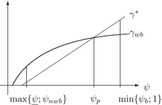
Fig. 1. Growth with versus without bubble.

Proof. SeeAppendix B. ■

A direct implication of this result is that an asymptotic bubbly BGP may exist if either the young households buy the bubble (

˜

b

∗

1

>

0) or take out some loans by being short-sellers of this asset to finance their investment in education (

˜

b

∗ 1

<

0).

Corollary 1shows that young households are short-sellers of the bubble if either the return of human capital

α

A or the time

cost per child

ψ

is sufficiently high. In the first case, the high return of human capital creates an incentive to finance education by selling short the liquid asset. In the second case, the quite high time cost per child incites households to have only a few number of children. Therefore, with the log-linear utility, the total rearing cost,

ψ

n∗

, is relatively low (see Eq. (36)). This low total time cost of rearing children incites the households to engage in loans when young to foster investments in education and redistributes income from the middle to the young age. On the contrary, in the second configuration of the corollary, i.e.

ψ

is low, the total time cost

ψ

n∗

is relatively high. Then, young households buy the bubble to finance this rearing cost of having children when adult.

6. Is a bubble productive?

We analyze now whether a bubble is productive. We say that it is productive when the growth factor at the asymptotic bubbly BGP is higher than at the bubbleless one. In this case, the positive valuation of the bubble raises the growth rate.

For such an analysis, the conditions for the existence of a bubbleless BGP, i.e. 1

> ψ > ψ

nwb and

µ < µ

nwb, and those

for the existence of an asymptotic bubbly BGP, i.e.

α <

β+2β2 1+2β+3β2,

A

>

A1 and

ψ < ψ <

min

{

ψ

b

;

1

}

, should all be satisfied

and should not imply an empty admissible interval for some parameters. Then, we could compare the asymptotic bubbly and bubbleless BGPs. We show the following:

Proposition 3. Let

ψ

p

≡

µ[

(1

−

α

)(1

+

µ + β

)

−

αβ

2

_]

(1

+

αβ

)(1

+

β + β

2

₊

µ

₎ (43)

1. Assume that A

>

A1,

µ < µ

nwb,

α

⩽ ₁+2ββ+β2 and

max

{

ψ; ψ

_nwb

}

< ψ

⩽

ψ

p hold. Then, the growth factor at

the asymptotic bubbly BGP is lower than at the bubbleless BGP (

γ

∗

⩽

γ

wb);

2. Assume that A

>

A1,

µ < µ

nwb,

α

⩽ _1+2β+ββ 2 and

ψ

p

< ψ <

min

{

ψ

_b

;

1

}

hold. Then, the growth factor at the asymptotic bubbly BGP is strictly larger than at the bubbleless BGP (

γ

∗

>

γ

wb).

Proof. SeeAppendix C. ■

As it is illustrated in Fig. 1,Proposition 3 shows that when the time cost per child

ψ

is relatively low, the economy without bubble is characterized by a higher growth rate than the economy with a bubble. On the contrary, when the time cost per child

ψ

is relatively high, the economy with bubble is characterized by a higher growth rate than the economy without bubble. In other words, if the time cost per child

ψ

is lower than the threshold

ψ

p,

the bubble is damaging for growth. If it is larger, the bubble or the positive valuation of the liquid asset is beneficial for growth. This last result is in accordance with the empirical facts underlying that episodes of bubble are associated with higher growth rates, as it is well documented inCaballero et al.(2006) orMartin and Ventura(2012).

While seminal papers likeTirole(1985) show that bubbles im-ply lower capital accumulation, various more recent contributions provide some mechanisms to reconcile the existence of rational bubbles with larger levels of capital (Fahri and Tirole, 2012;

Kocherlakota,2009;Martin and Ventura,2012;Miao and Wang,

2018;Raurich and Seegmuller,2015). In models with endogenous growth,Grossman and Yanagawa(1993) show that the existence of a bubble reduces the growth rate, but more recent results show that bubbles may be in accordance with higher growth rates.

Olivier(2000) highlights that a bubble on equity raises the value of firms, which promotes firm creation and growth. On the con-trary, bubbles on unproductive assets have the same effect than inGrossman and Yanagawa(1993).Hirano and Yanagawa(2017) discuss the existence of bubbles in a model with heterogeneous investment projects and borrowing constraints. These authors are especially concerned with the interplay between growth and the existence of bubbles according to the degree of financial imperfections.

Our paper differs from these last two contributions. In con-trast toOlivier(2000), growth is enhanced by the existence of a bubble even if the bubble is on an unproductive asset. Therefore, the mechanism that allows to have a productive bubble in our framework is different. We also depart from Hirano and Yana-gawa(2017) since we do not consider heterogeneous investment projects and do not discuss the results according to the level of financial frictions.

By inspection of Corollary 1 and Proposition 3, the bubble pushes up growth if

ψ >

max

{

ψ

_p

,

ψ}

ˆ

. In this configuration, households are short-sellers of the bubble to have loans from middle-age agents used to finance investments in education. Hence, the bubble promotes human capital and, therefore, growth. It is however interesting to note that we can have

ψ

p lower

than

ˆ

ψ

.10This means that for

ψ

p

< ψ <

ˆ

ψ

, we can have a higher growth of the ratio of human capital over labor at the asymptotic bubbly BGP than at the bubbleless one (

γ

∗

_{> γ}

wb) even if young

households are not short-sellers of the speculative asset. This is in contrast with Raurich and Seegmuller (2015, 2017) who study the existence of rational bubbles in overlapping generations economies with three period-lived households, vintage capital and exogenous growth. In both papers, capital is higher at the bubbly than at the bubbleless steady state only if either young or adult households are short-sellers of the bubble. Here, we obtain a different result, which means that the mechanism for the existence of a productive bubble is different than in these two papers.

Our model with endogenous fertility and rational bubble also allows us to refer to the debate on the link between population size and the value of assets (Abel,2001;Geanakoplos et al.,2004;

10 _{We note that when Proposition 3applies, it corresponds to case 2 of}

Corollary 1, because ₁ β

+2β+β2 < β+β2

1+2β+2β2. Then, using(42)and(43),ψp<ˆψ requiresµ <1−α(1−_αα₍₁)+−αα2)(β+β2).

Fig. 2. The interplay between bubble, fertility and growth.

Poterba, 2005), which explains that asset price is higher when the relative number of savers is larger. In particular,Geanakoplos et al. (2004) consider an overlapping generations model with three-period lived agents and show this relationship in a model where the relative number of savers is directly related to the ratio of middle-age over young households.

Of course, to make a link between population size and asset price level, one needs to focus on the comparison of quite long periods. Therefore, we can contribute to this debate comparing the asymptotic bubbly and bubbleless BGPs and focusing on the price of the liquid asset. Obviously, the price of this asset is larger with the bubble than without. In the next corollary, we consider the range of parameter values for which the bubble is productive and we first make sure that, at the asymptotic bubbly BGP, middle-age households hold a larger amount of the bubble than young ones. Then, observing that the ratio of middle-age over young households is given by MYt

≡

Nt−1

/

Nt

=

1

/

nt, we

denote by MY∗

and MY_wb the value of this ratio evaluated at

the asymptotic bubbly and bubbleless BGPs, respectively, and we compare them:

Corollary 2. Assume that A

>

A1,

µ < µ

nwb,

ψ

p

< ψ <

min

{

ψ

b

;

1

}

and

α

⩽ ₁+2β+ββ 2 hold. Then, we have

˜

b

∗ 2

>

n ∗

˜

b ∗ 1,

γ

∗

_{> γ}

wband n∗

<

nwb, which means that MY∗

>

MYwb.

Proof. SeeAppendix D. ■

This corollary ensures first that middle-age households hold a larger amount of the bubble than young agents living at the same period (

˜

b ∗ 2

>

n ∗

˜

b ∗

1). Therefore, a higher MY is a relevant measure to argue that more traders buy the speculative asset. Then, comparing the asymptotic bubbly and bubbleless BGPs, we have not only that

γ

∗

> γ

wb, but also MY∗

>

MYwb and the

price of the speculative asset is of course larger at the asymptotic bubbly BGP, since it is zero at the bubbleless one. This cor-roborates the theoretical and empirical findings ofGeanakoplos et al.(2004) on the link between demography and asset prices. The basic mechanism they focus on is the following: the lower price of asset is explained by a relative lower number of savers, measured by a smaller ratio of adult over young households, which reduces the demand of asset. In our model, we associate the asset price to the bubble and a larger ratio of adult over young households means that the main buyers of the speculative asset are relatively more. Hence, we observe in the long run the same link thanGeanakoplos et al.(2004) between the asset price and the demography.

7. Crowding-out versus crowding-in effect

To explain the economic mechanism that allows to have larger growth when there is a bubble, we next highlight three main ingredients that relate the explanation to the value of the time cost per child

ψ

.

1. The liquid asset allows to smooth consumption along the life-cycle. At middle-age, a household buys the bubble (

˜

b

∗

2

>

0) to transfer purchasing power to the old age. Using

˜

b

∗

1, the household uses the liquid asset to take out some loans or save for adulthood. As already discussed in the previous section, we learn from Corollary 1 and

Proposition 3that a growth enhancing bubble at the BGP is not equivalent to have

˜

b

∗

1

<

0, i.e. young households are short-sellers of the bubble to get some loans. Indeed, there is a value

ˆ

ψ

such that

˜

b

∗ 1

>

0 if

ψ <

ˆ

ψ

,

˜

b ∗ 1

=

0 if

ψ =

ˆ

ψ

, while

˜

b ∗ 1

<

0 if

ψ >

ˆ

ψ

.

2. In Corollary 2, we have shown that if

γ

∗

_{> γ}

wb, we get

n∗

<

n_wb. Now, without comparing the growth factors, we

deduce, using (17)and (36), that n∗

_<

n_wb if and only if

ψ > ψ

n, with

ψ

n

≡

µ

(1

−

α

)

1

+

β

(

α + β

) (44)

3. Recall now that

γ

denotes the growth factor of human capital per unit of labor. It is often more usual to define the growth factor of human capital per capita (or GDP per capita). This last one is defined by Ht

/

Nt

=

htLt

/

Nt

=

ht(1

−

ψ +

1

/

nt). On a BGP, since n is constant, the growth

factor of human capital per capita is also equal to

γ

and the growth factor of human capital is defined by

γ

H

≡

Ht+1 Ht

=

ht+1 ht Nt+1 Nt

=

γ

n

Using(32),

γ

H

=

α

A

≡

γ

H∗at the asymptotic bubbly BGP

and, using(16)and(17),

γ

H

=

_ψ(1+µααβA)+αµ

≡

γ

H,wbat the

bubbleless BGP. We deduce that

γ

∗

H

> γ

H,wbif and only if

ψ > ψ

H, with

ψ

H

≡

µ

(1

−

α

)

1

+

αβ

(45)

Using(42),(44)and(45), we have that

ψ

n

<

ˆ

ψ < ψ

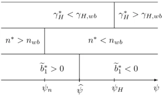
H.11This

allows us to drawFig. 2, which is useful to understand why the bubble can increase growth of GDP per capita. As follows from this figure, there are three main configurations according to the value of

ψ

:

ψ < ψ

n,

ψ

n

< ψ < ψ

H and

ψ > ψ

H.

Before studying these different configurations, it is useful to note that since

γ = γ

H

/

n, the threshold value

ψ

p above which

γ

∗

_{> γ}

wbbelongs to (

ψ

n

, ψ

H). Of course,

γ

∗

> γ

wbfor

ψ

⩾

ψ

H

and

γ

∗

_{< γ}

wbfor

ψ

⩽

ψ

n.

1.

ψ < ψ

n: Crowding-out effect

Since

ψ

is small, the number of children and the total time cost of rearing children

ψ

n are high, whether or not

the bubble exists (see(17)and(36)). Therefore, when the liquid asset is positively valued, the households use it to transfer income to middle-age and cover rearing expenses. This reduces investment in education, which implies less human capital and a lower growth. This also reduces the cost of having children

ψw

t+1 in terms of consumption, which explains that population growth is higher at the asymptotic bubbly BGP than at the bubbleless one. 2.

ψ

n

< ψ < ψ

H: Indeterminate crowding effect

Both

ψ

and

ψ

n∗take intermediate values. The main mech-anism at stake is clearly different than in the previous configuration. To understand what happens, let us assume

ψ =

ˆ

ψ

. At the asymptotic bubbly BGP, young households

11 _{One can further note that underProposition 3, max{ψ; ψ}

nwb}< ψnand ψH <min{ψb;1}, which means that the critical values we focus on belong to the interval ofψ considered inProposition 3.

neither buy, nor sell the bubble, i.e.

˜

b

∗

1

=

0. Since

˜

b

∗ 2

>

0, a middle-age household saves to finance consumption when old and reduces the child related expenses by having a lower number of children at the asymptotic bubbly BGP. Then, investment in education e, whose returns are used to finance future expenditures at adulthood, can be higher or lower at the asymptotic bubbly BGP than at the bubbleless one because of two opposite effects: on the one hand, fewer child related expenses have to be covered; on the other hand, the purchase of the bubble to finance consumption when old has to be financed.

3.

ψ > ψ

H: Crowding-in effect

Since

ψ

is large enough, the number of children and

ψ

n

are relatively low, whether or not the bubble exists. There-fore, the main mechanism is exactly the opposite one than in the first configuration. In this case, the labor supply when adult is high and the cost of rearing children to be financed is low. When the bubble exists, there is a transfer of resources from the adult to the young age. The young household becomes a short-seller of the bubble, to get loans and increase investments in education. Therefore, this enhances human capital and growth at the asymptotic bubbly BGP. This larger growth also implies a larger cost of having children

ψw

t+1in terms of consumption. Therefore, population growth is lower when there is a bubble.

8. Concluding remarks

We develop a model where a liquid asset (bubble) is used to finance two types of expenditures, education and costs of rearing children. If the time cost per child

ψ

is low, the household has a large number of children, meaning that the total time cost

ψ

n is high. In this case, the bubble is mainly used to finance

child related expenses during adulthood instead of investment in education during youth. The bubble is a mean of saving and growth is lower with a bubble than without. If

ψ

is high, we have the opposite. The total time cost of having children

ψ

n is

low and the bubble is a mean to get loans to finance education, which enhances human capital and growth.

The comparison between equilibria with and without bubble can also be interpreted in terms of financial development. Such an interpretation of our results may contribute to the literature studying the link between financial development and growth.12 In our framework, the bubbly equilibrium describes an economy where financial markets are more developed since there is an adding traded asset valued on such a market. Under this in-terpretation, our model suggests that financial development is beneficial for growth only under some circumstances, i.e. if

ψ

is high enough.

Appendix A. Proof ofProposition 2

We have n∗

<

1

/ψ

if and only if

ψ > ψ

, where this inequality ensures that

ψ > µ/

(1

+

β + β

2

+

µ

). Then, using (39), we immediately see that B∗

_>

0 if and only if

ψ < ψ

b. We also

note that

ψ <

1 because

µ <

1 and

ψ < ψ

b is equivalent

to

α <

β+2β2

1+2β+3β2 . Of course, there is sustained growth because

A

>

A1.

Let us focus now on the stability properties. Even if (

γ

∗

_,

B∗

_,

0) is an asymptotic BGP, it is important to note that from the mathematical point of view, (

γ

t

,

Bt

, λ

t)

=

(

γ

∗

,

B∗

,

0) is a steady

state of the dynamic system(29)–(31). Therefore, to analyze the

12 _{SeeLevine(2005) for a survey andMadsen and Ang(2016) for a recent}

contribution.

stability properties of the equilibrium (

γ

∗

_,

B∗

_,

0), we use standard mathematical tools.

Differentiating the dynamic system(29)–(31)in the neighbor-hood of the BGP (

γ

∗

_,

B∗

_,

0), we obtain a linear system of the following form:

dBt+1

=

a11dBt

+

a12d

γ

t

+

a13d

λ

t

d

γ

t+1

=

a21dBt

+

a22d

γ

t

+

a23d

λ

t

d

λ

t+1

=

a33d

λ

t

Therefore, the characteristic polynomial can be written P(

η

)

≡

(a33

−

η

)(

η

2

−

T

η +

D)

=

0, with T

=

a11

+

a22 and D

=

a11a22

−

a12a21. We immediately deduce that one eigenvalue is given by

η

1

=

a33

=

1

/γ

∗

∈

(0

,

1). To determine the other eigenvalues, we compute the terms aij, with

{

i

,

j

} = {

1

,

2

}

:

a11

=

1

−

B∗

α

A

∂

˜

b ∗ 1

/∂γ

t+1 (A.1) a12

= −

B∗ n∗

∂

nt

∂γ

t

+

B ∗

α

A

∂

˜

b ∗ 1

/∂γ

t+1

(

˜

b ∗ 1

∂

nt

∂γ

t

+

∂

˜

b ∗ 2

∂γ

t

)

(A.2) a21

=

γ

∗

α

A

∂

˜

b ∗ 1

/∂γ

t+1 (A.3) a22

= −

γ

∗

α

A

∂

˜

b ∗ 1

/∂γ

t+1

(

˜

b ∗ 1

∂

nt

∂γ

t

+

∂

˜

b ∗ 2

∂γ

t

)

(A.4) The minor D is given by

D

=

γ

∗

α

A

∂

˜

b ∗ 1

/∂γ

t+1

(

B∗ n∗

∂

nt

∂γ

t

−˜

b∗ 1

∂

nt

∂γ

t

−

∂

˜

b ∗ 2

∂γ

t

)

Using n∗

₌

_α

A

/γ

∗ and B∗

₌

n∗

˜

b ∗ 1

+˜

b ∗ 2, we obtain D

=

1 (n∗₎2

∂

˜

b ∗ 1

/∂γ

t+1

(

˜

b ∗ 2

∂

nt

∂γ

t

−

∂

˜

b ∗ 2

∂γ

t n∗

)

From(26)and(27), we get

∂

nt

∂γ

t

= −

µ/ψ

1

+

β + β

2

₊

µ

α

A

γ

2 t

∂

˜

b ∗ 2

∂γ

t

= −

β

2

_α

_A 1

+

β + β

2

₊

_µ

(1

−

α

)A

γ

2 t

Using(36)and(38), we deduce that D

=

0. This means that one eigenvalue is zero, i.e.

η

2

=

0. Using now(26),(27),(A.1)and

(A.4), T rewrites T

=

1

−

B ∗

α

A

(

αA γ∗

+

1

)

_∂ ˜b ∗ 1 ∂γt+1

We easily derive from(25)that

∂

˜

b ∗ 1

∂γ

t+1

= −

1

−

(1

−

ψ

)

µ/ψ

1

+

β + β

2

₊

µ

−

1 1

+

β + β

2

₊

µ

1

−

α

α

<

0 We deduce that the last eigenvalue is given by

η

3

=

T

>

1.

To better understand the dimension of the stable manifold and the type of indeterminacy generated by the model, the stable solution of the dynamic system is given by

Bt

=

v

11

ξ

1

η

t1

+

v

21

ξ

2

η

2t

+

B ∗ (A.5)

γ

t

=

v

12

ξ

1

η

t1

+

v

22

ξ

2

η

2t

+

γ

∗ (A.6)

λ

t

=

v

13

ξ

1

η

1t

+

v

23

ξ

2

η

2t (A.7) for all t ⩾1. The parameter

ξ

iis a constant and

v

i

=

(v

i1

, v

i2

, v

i3

)

is the eigenvector associated to the eigenvalue

η

i, for i

=

1

,

2. The

eigenvectors are defined by

a21

v

i1

+

(a22

−

η

i)

v

i2

+

a23

v

i3

=

0 (A.9)

(a33

−

η

i)

v

i3

=

0 (A.10)

For i

=

1, we have

η

1

=

a33

=

1

/γ

∗. Eq.(A.10)is satisfied for

v

13

̸=

0. Given the value of

v

13, Eqs.(A.8)and(A.9)rewrite (a11

−

a33)

v

11

+

a12

v

12

= −

a13

v

13 (A.11) a21

v

11

+

(a22

−

a33)

v

12

= −

a23

v

13 (A.12) There exists a unique solution (

v

11

, v

12)

̸=

(0

,

0) at this system because (a11

−

a33)(a22

−

a33)

−

a12a21

=

a233

−

a33T

+

D

=

a33(a33

−

T )

<

0.

For i

=

2, we have

η

2

=

0. Using(A.10), we get

v

23

=

0. Then, using(A.8)and(A.9), we deduce that

v

21

=

v

22

=

0.

Using these results, Eqs.(A.5)–(A.7)become

Bt

=

v

11

ξ

1

η

1t

+

B ∗

, γ

t

=

v

12

ξ

1

η

1t

+

γ

∗

, λ

t

=

v

13

ξ

1

η

t1 or, equivalently

γ

t

−

γ

∗

=

v

12

v

13

λ

t

,

Bt

−

B ∗

=

v

11

v

13

λ

t for all t⩾1.

This means that for all periods t ⩾ 1, the stable manifold is one-dimensional. Moreover, the stable manifold is transversal to the subspace spanned by the jump variables, as we have shown that the eigenvector associated to the eigenvalue

η

1

=

a33 is different from zero.

However, because one eigenvalue is equal to 0, the stable manifold is two-dimensional at t

=

0, but the economy jumps at t

=

1 to the one dimensional stable submanifold described above. There is a form of local indeterminacy because the stable manifold has a dimension strictly higher than one at t

=

0.

Appendix B. Proof ofCorollary 1 Using (37), we see that

˜

b

∗

1

<

0 if and only if

ψ >

ψ

ˆ

. We further have that

ˆ

ψ < ψ

b,

ˆ

ψ <

1 is ensured by

µ <

1 and

ˆ

ψ > ψ

if and only if

α <

β+β2

1+2β+2β2. If this last inequality is

not satisfied, we have

ˆ

ψ

⩽

ψ

. Since β+β

2

1+2β+2β2

<

β+

2β2

1+2β+3β2, the

corollary immediately follows.

Appendix C. Proof ofProposition 3

We first take into account the conditions for the existence of a bubbleless BGP, i.e.

µ < µ

nwb and

ψ > ψ

nwb. They are

compatible with the conditions for the existence of an asymptotic bubbly BGP if

ψ

nwb

< ψ

b, which is satisfied if and only if

α

(1

+

2

β + β

2₎

₋

_{β +}

₂

_αβ

2₍

_{α −}

₁₎

_<

_{0. This last inequality} is ensured for

α

⩽ _1+2β+ββ 2, which implies that

α <

β+

2β2

1+2β+3β2.

Therefore, the bubbleless and asymptotic bubbly BGP coexist if max

{

ψ; ψ

nwb

}

< ψ <

min

{

ψ

b

;

1

}

.

Using (16) and (34), we note that

γ

∗

_{> γ}

wb if and only if

ψ > ψ

p. We can further show that

ψ

p

<

1 and

ψ

p

< ψ

bbecause

α

⩽ _1+2β+ββ 2. Moreover, using(18),(41)and(43), we can further

show that under

α

⩽ _1+2β+ββ 2, we have

ψ

p

>

max

{

ψ; ψ

nwb

}

.

Indeed,

ψ

p

> ψ

is equivalent to

(1

+

β + β

2)

[

β − α

(1

+

2

β + β

2)

]

> µ[α

(1

+

2

β + β

2)

−

(

β + β

2)

]

and

ψ

p

> ψ

nwbto

µ[β − α

(1

+

2

β

)

]

>

(1

+

β

)

[

α

(1

+

2

β + β

2)

−

β]

Both inequalities are satisfied under

α

⩽ _1+2β+ββ 2. This means that

max

{

ψ; ψ

_nwb

}

< ψ

_p

<

min

{

ψ

_b

;

1

}

and the proposition follows.

Appendix D. Proof ofCorollary 2 Using (36)–(38), the inequality

˜

b

∗ 2

>

n ∗

˜

b ∗ 1 is equivalent to

ψ > ψ

n, with

ψ

n

≡

µ

(1

−

α

) 1

+

αβ + β

2

Using now(43),

ψ

p

> ψ

nis equivalent to

β − α

(1

+

2

β + β

2)

+

µ

(1

−

α

)

>

0 which is always satisfied for

α

⩽ ₁+2ββ+β2.

Using Proposition 3, we have

γ

∗

_{> γ}

wb. Using(17)and(36),

we easily deduce that n∗

<

n_wb. This means that MY

∗

>

MY_wb.

References

College Board, 2016. Trends in Student Aid 2016. In: Trends in Higher Education Series.

Abel, A.B., 2001. Will bequests attenuate the predicted meltdown in stock prices when baby boomers retire. Rev. Eco. Stat. 83, 589–595.

Acemoglu, D., Guerrieri, V., 2008. Capital deepening and non-balanced economic growth. J. Political Econ. 116, 467–498.

Aguiar, M., Hurst, E., 2005. Consumption versus expenditure. J. Political Econ. 113, 919–948.

Alonso-Carrera, J., Raurich, X., 2015. Demand-based structural change and balanced economic growth. J. Macroecon. 46, 359–374.

Alonso-Carrera, J., Raurich, X., 2018. Labor mobility, structural change and economic growth. J. Macroecon. 56, 292–310.

Avery, C., Turner, S., 2012. Student loans: do college students borrow too much - or not enough? J. Econ. Perspect. 26, 165–192.

Benhabib, J., Rogerson, R., Wright, R., 1991. Homework in macroeconomics: household production and aggregate fluctuations. J. Political Econ. 99, 1166–1187.

Caballero, R.J., Fahri, E., Hammour, M.L., 2006. Speculative growth: hints from the U.S. economy. Amer. Econ. Rev. 96, 1159–1192.

de la Croix, D., Doepke, M., 2003. Inequality and growth: why differential fertility matters. Amer. Econ. Rev. 93, 1091–1113.

de la Croix, D., Michel, P., 2007. Education and growth with endogenous debt constraints. Econom. Theory 33, 509–530.

Duernecker, G., Herrendorf, B., 2015. On the allocation of time - a quantitative analysis of the U.S. and France. CESifo Working Paper 5475.

Dynarski, S.M., 2014. An economist’s perspective on student loans in the United States. Brookings Institution Working Paper.

Fahri, E., Tirole, J., 2012. Bubbly liquidity. Rev. Econom. Stud. 79, 678–706. Frankel, M., 1962. The production function in allocation and growth: a synthesis.

Amer. Econ. Rev. 52, 996–1022.

Galor, O., 2005. From stagnation to growth: unified growth theory. In: Aghion, P., Durlauf, S.N. (Eds.), Handbook of Economic Growth. North-Holland, Amsterdam, pp. 171–293.

Geanakoplos, J., Magill, M., Quinzii, M., 2004. Demography and the long-run predictability of the stock market. Brook. Pap. Econ. Act. 1, 241–325. Gente, K., Leon-Ledesma, M., Nourry, C., 2015. External constraints and

endoge-nous growth: why didn’t some countries benefit from capital flows? J. Int. Money Finance 56, 223–249.

Gronau, R., 1986. Home production - a survey. In: Ashenfelter, O., Layard, R. (Eds.), Handbook of Labor Economics. North-Holland, Amsterdam, pp. 274–304.

Grossman, G.M., Yanagawa, N., 1993. Asset bubbles and endogenous growth. J. Monet. Econ. 31, 3–19.

Hirano, T., Yanagawa, N., 2017. Asset bubbles, endogenous growth, and financial frictions. Rev. Econom. Stud. 84, 406–443.

Hurst, E., 2008. The retirement of a consumption puzzle. NBER Working Paper 13789.

Jones, L.E., Tertilt, M., 2008. An economic history of fertility in the US: 1826-1960. In: Rupert, P. (Ed.), Frontiers of Family Economics. Emerald Group Publishing, pp. 165–209.

Kocherlakota, N., 2009. Bursting Bubbles: Consequences and Cures. Mimeo, Federal Reserve Bank of Minneapolis.

Kongsamut, P., Rebelo, S., Xie, D., 2001. Beyond balanced growth. Rev. Econom. Stud. 68, 869–882.

Levine, R., 2005. Finance and growth: theory and evidence. In: Aghion, P., Durlauf, S.N. (Eds.), Handbook of Economic Growth. North-Holland, Amsterdam, pp. 865–934.