A comparison of the velocity fields associated with vorticities of three different origins

A Comparison of the Velocity Fields Associated

With Vorticities of Three Different Origins

by

Gilbert W. Chiang

-Submitted to the Department of Aeronautics and Astronautics

in partial fulfillment of the requirements for the degree of

Master of Science

at the

MASSACHUSETTS INSTITUTE OF TECHNOLOGY

June 1992

©

Massachusetts Institute of Technology 1992. All rights reserved.

Author

Department of Aeronautics and Astronautics

May 18, 1992

Certified by

Professor Eugene E. Covert

Thesis Supervisor

Accepted by

Professor Harold Y. Wachman

Chairman, Department Graduate Committee

AeT

I

MASSACHUSETTS INSTITUTE

Abstract

Experiments are conducted to study the characteristics of flow behind three sources of vorticity. These are a vortex tube, and two wings of high and low aspect ratios. Only the measurements behind the two wings are useful. The results are in good agreement with theoretical predictions and with available experimental data. A relation between circulation and centerline axial velocity is derived for the low aspect ratio wing.

Acknowledgments

My first thanks goes to Prof. Eugene Covert for giving me the opportunity to work in the Aeronautical field. I will always be grateful for his guidance and patience.

I also wish to thank the McDonnell Aircraft company for their funding, without which this project would not have been possible.

Also without my family's support I would not be here.

Finally, I am forever in debt to Monika Gorkani for her excellent typing of this thesis, and her wonderful support throughout.

Contents

1 Introduction 10

2 Literature Review 12

3 Theory 17

4 Equipment 25

4.1 The W ind Tunnel ... 25

4.2 Sources of Vorticity ... ... 27

4.2.1 The Vortex Tube ... 27

4.2.2 W ings . . . .. . 27

4.3 5-hole Pitot Probe ... 30

4.3.1 Description . . . .. . . . .. . . . 30

4.3.2 Probe Calibration ... 32

4.3.3 Use of Calibrated Probe ... 35

4.4 Constant Temperature Crossed Hot Wire Anemometer ... 36

4.4.1 Description, and Theory of Operation . ... 36

4.4.2 Calibration and Use ... 37

5 The Vortex Tube 39 6 The High and Low Aspect Ratio Wings 49 6.1 Method of Data Analysis ... ... 49

6.2.1 Circulation .. . . .. . .. . . . . . .. 54

6.2.2 Axial Velocity Profiles ... 56

6.2.3 The Wake ... 59

6.2.4 Vortex Core Positions ... 61

6.3 Measurement Errors ... ... 62

6.4 D iscussion . . . . . . .. . . . . .. 66

6.4.1 Circulation .. .. ... .... .. .. ... .. .. .. . . .. 66

6.4.2 Centerline Axial Velocity Defect . ... 68

6.4.3 The W ake ... .... .. .. 68

6.4.4 Vortex Core Positions ... 69

List of Figures

2-1 Horseshoe vortex system [26] . . . . 2-2 Conical vortex growth [25] ...

3-1 Rankine vortex azimuthal velocity profile . . . . 3-2 Burger vortex ... .. .. 3-3 Example of q-Vortex axial velocity profile . . . . 3-4 Definition of variables in flow field with two potential vorticies

4-1 4-2 4-3 4-4 4-5 4-6 5-1 5-2 5-3 5-4 6-1 6-2 6-3 6-4 6-5

Sketch of wind tunnel plan view . . . . . Wind tunnel calibration ...

Vortex tube schematic ...

Wing geometry in tunnel working section

5-hole pitot probe geometry ... X-wire probe ...

Conditions for parallel smoke flow . . . .

5-hole pitot probe results . . . . Hot wire results, radial inflow ... Hot wire results, no radial inflow . . . .

Definition of variables used in data analysis . . .

Paths of integration for calculation of circulation .

Traverse geometries ...

High AR wing at a = 100 - axial velocity profiles Example of calibration data . . . .

. . . 51 52 ... 53 . . . 57 . . . 64 . . . . . 26 . . . . 28 . . . . 29 . . . . . 31 . . . . 33 . . . . 37 . . . . . . . . . 40 . . . . . 43 . . . . 45 . . . . . 47

C'f;(lrrii1~trrn siinma~rv for delta wine at I = 2

6-7 Circulation summary for rectangular wing at = 2 . ... 70

Nomenclature

a angle of attack

ap probe pitch angle

OP, probe yaw angle

7 vortex strength per unit length

7, angle of probe to flow

F circulation

I Gamma function

0 polar coordinate angle

polar coordinate angle

OP probe roll angle

AR aspect ratio

b wing span

c wing root mean chordlength

CL coefficient of lift

CLa lift curve slope

e distance behind wing where a vortex is rolled up

KI,~3,q* probe calibration coefficients

1 vector describing position along a vortex line

P; pressures read from probe holes

r radius from vortex centerline

r vector describing point in flow field

Rec Reynolds number based on chordlength

re effective radius from vortex centerline

s semi-span of wing

s vector along a contour path for a line integral

s' trailing vortex semi-spacing

u radial velocity component

U, freestream velocity

V velocity vector

vo azimuthal velocity component

w axial velocity component

x distance downstream of triangular wing apex

y spanwise position, measured from wing midspan

Chapter 1

Introduction

Advances in aircraft technology have led to the generation of more manoeuvrable aircraft. These manoeuvres require the aircraft to fly at very high angles of attack. Accompanying this is the threat of vortex breakdown, an unsteady transformation of the vortex above the wing, which causes excessive loading and fatigue on the aircraft structure. Prediction of the onset of breakdown is thus of great interest. Although the study of vortex breakdown has been pursued for over 30 years it has

not, to date, produced a satisfactory model for the phenomenon. The theories so far have involved hydrodynamic instability [1], critical states [2], standing waves [3], and solitons (nonlinear wave packets) [4]. None of these models adequately describe

breakdown. Numerical simulations have been successfully used [5, 6, 7], but the method is limited by computing power and its associated cost.

This study, motivated and funded by McDonnell Aircraft Company,was aimed at experimentally providing a data base to describe the occurrence and location of

breakdown under various vortex and flow conditions. Thus without fully understand-ing it, breakdown could still be predicted.

The sources of vorticity used were:

1. A wing of high aspect ratio (AR) ;

2. A wing of low aspect ratio ; and

These are described in greater detail in section 4.2.

The vorticies shed by each of these sources were studied so that they could be parameterized for later use in a breakdown study.

Chapter 2

Literature Review

The study of flow behind wings dates back to Prandtl [7] and Lanchester [8] in the first two decades of this century. The most fundamental ideas on tip vorticies shed

by high aspect ratio (AR) wings are well known. The far-field case is the most simple where the velocity field is generated by essentially two parallel quasi-2D vortex lines. In the near-field the velocity field cannot be described by such a simple method

because the vortex is rolling up and the circulation is changing rapidly. The solution is obtained by considering the velocity contribution from the bound vortex over the wing and from the two line vortices with their associated strengths y7() (figure 2.1).

The Biot-Savart Law provides the integral equation for each contribution :

1 _Y (1)

[dlX r]

Application of this theorem, known as Prandtl's lifting line, provides approxi-mate solutions for high aspect ratio of wings . The above method does not take into account the trajectory of the vortex lines. Spreiter and Sachs [9] performed

experi-ments to determine the vortex trajectories behind wings, both of high and low AR.

They found that the path of the vortex, as it rolled up, remained approximately in the y - z plane. The spanwise position was approximated to fit both the result of Kaden [10] in the near field behind the wing, and the asymptote y = s' in the far

field. Their result was

y =

s

-

(s

-

')tanh( )

with e = K(R)b; K - 0.28;

3

Accompanying experiments conducted on vortex trajectories were studies of the downwash [9, 11] and of the wake [11]. These results were needed in tail-plane design for aircraft. More recent developments focused on the core region of vorticies. Several models describing vortex cores were developed. Moore and Saffman [13] provided a model for the flow in the core of trailing tip vorticies. Where the wing loading varied as the square root of the distance from the wing tip (such as in elliptic loading) then the azimuthal velocity near the center of the vortex was given by

5 4vx 3 -U,r 2

v(r, x) = r( )r( )-'M(; 2;4x

4 U0

4 4vx

with / = aUo (1 + ~ ; r is the Gamma function; and M is the confluent hypergeometric function.

Flow over a low AR wing differs from that over one of high AR because of the way in which the vortex forms. The flow separates from the leading edge forming a vortex sheet which rolls up into a vortex above the wing. This vortex grows conically with downstream distance (figure 2.2). Stewartson and Hall [12] generated a model for this by assuming two core regions - a viscous inner core and a inviscid outer core

two core regions were then matched to produce the following results: u 1 -= -Cr'

UIo

2

v/

1

Uoo

where r' is the radius; dimensionalized by the outer core radius;

K is a shape factor; and C is a velocity magnitude factor.

The experimental study of vortex cores is of interest for two reasons. Firstly, the theoretical modeling of the velocity distribution is useful only if it matches ex-perimental measurements. However, the vortex core is difficult to measure because of its tendency to deflect in the presence of any probes, or even undergo local vortex breakdown [15]. Furthermore, velocities in the vortex core are often very unsteady.

Behaviour of vortex core flow is dependent upon the position of the vortex down-stream of the wing. Green and Acosta [15] found that in the near field behind the wing (0-2 chordlengths downstream) the flow was highly unsteady even though the vortex was fully rolled up. As the vortex grew and moved downstream, the unsteadiness of the azimuthal velocity was significantly lowered but the axial velocity fluctuations still remained high. At a high angle of attack (10o) the axial velocity was found to have a long-wavelength unsteadiness. Bandyopadhyay et al [16] also found a similar effect, describing the core to have "... a wavelike character... [with]... intermittent patches of highly turbulent and partially relaminarized fluid...". Such character readily explains the fluctuations measured by Green and Acosta.

Vortex cores also tend to "wander". Such meandering is not modeled theo-retically. Furthermore, it affects the average velocity measured by any instrument, intrusive or not. Baker et al [17] used a 2D Gaussian probability distribution to model the position of the vortex due to its meandering, and found that in their earlier

ex-experiments, the measured maximum azimuthal velocity in the vortex core had been measured at only - 70% of its correct value, and that the actual core radius was only

30% of its measured value. They noted that such meandering occurred only after - 2

chordlengths downstream of the airfoil, where the vortex no longer grew rapidly.

Secondly, vortex cores are of interest because it is within this viscous region that vortex breakdown (VBD) is initiated. The flow in the core decelerates due

to viscosity or due to adverse pressure gradients in the surrounding potential field, until it stagnates where upon the core undergoes the rapid expansion that is typical of VBD. There is still considerable disagreement as to the cause of its occurence. Comprehensive reviews on VBD have been written [17, 18, 19] and will not be repeated here.

circulation

a)SnDUlsl~On

(•sm uun ,,

1l

Figure 2-1: Horseshoe vortex system [26]

Figure 2-2: Conical vortex growth [25] I

Chapter 3

Theory

The most fundamental representation of vortex flow is given by the Navier-Stokes equations. The steady inviscid axisymmetric assumption yields:

Continuity: Ou U aw r rt-t -Or r Oz

0 (V.V=o)

u

au

v

By assuming a quasi 2-D model (ie. -2 _{= 0) then the 0-momentum equation}

a

u

S--Br

+ w-z

8z

yields the azimuthal velocity equation

By defining circulation, F, such that

1

vo oc

-r (3.2)

(3.3)

r = . - ds

then the potential field solution is found as

r

v(r) = 2rr

_2rr

As r -+ 0, then v(r) -- oo, which is not physically possible. The assumption of

potential flow fails in this region.

Several models are available to overcome this problem. The simplest is the

Rankine vortex model [24]. It describes the vortex in two parts, as shown in equation 3.1 and in figure 3.1:

r > ro

r < r.

(3.5)

where K = 27rF describes the vortex circulation.

The model is a two dimensional one and does not describe the axial velocity

compo-nent of the vortex flow. It is clearly inadequate.

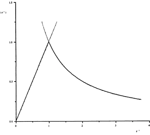
A much improved model which includes an axial velocity description is the

Burger vortex model [24]. It is able to fit most experimentally measured

circumferen-L_r

V rK

v (r) ='

v(r')

1.0

0.

00

0 1 2 3 4

Figure 3-1: Rankine vortex azimuthal velocity profile

tial velocity profiles well. However, its axial velocity profile is limited in application.

The model's equations are :

v(r)

=

-

(3.6)

r

w(r) = w1 + w2e-lr2 (3.7)

where a = - =

It should be noted that as r -- 0 then v(r) -+ v, and as r -- oc then v(r) -- g

Thus in the inner and outer limits the Burger model approach those of the Rankine model.

The model is still only 'quasi' two dimensional ('quasi' because it is independent

of axial position, yet it does describe a velocity in the axial direction). Furthermore, it is able to model only a vortex with pure velocity excess or defect in its core,

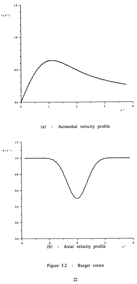
exemplified in figure 3.2.

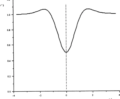
The most appropriate model is the q-vortex model [24] with describing equations:

v(r, x) K()(1 - e- x)r) (3.8)

w(r,x) = wl(r,x) + w2(r,x)e&(x)r- 2 (3.9)

This model is clearly three dimensional, and allows for such axial velocity profiles shown in figure 3.3.

The vortex profiles in this work were all measured in a single plane behind the wings, and thus the information is not available for a true q-vortex fit. The simplified

model used will be

v(r) = -(1 - e-ar) (3.10)

r

w(r)

wi(r)

+

w

(r)e-2

(3.11)

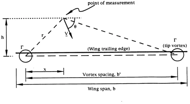
Analysis of the data in these experiments requires some modeling of the vortex flow behind wings. Two assumptions are made. Firstly, that at 2 chordlengths downstream of the trailing edge, the vorticies are nearly fully rolled up; and secondly that at this station, the vortex lines are nearly parallel. The model considers a pair of irrotational counter-rotating streamwise vorticies. The potential fields of the two vorticies interact such that the streamlines in the crossplane projection are not circular, as they would be for a single line vortex. Instead the equations describing the cross-plane velocity at any particular point in flowfield are

Kb

(x2

+

h2)((b- ~)

_{+ h}

₎

(b

- x)h - hz

where each variable is defined in figure 3.4. The total head is then

1

H = -p(v _o + w2) 2

Defining a total velocity, vt, so that

2H

P

then using equation 3.11 an asymptotic approximation near r = 0 yields

(3.12) (3.13) (3.14)

t2/

- (rbr')2 _ r'2

where wo is the nondimensional centerline axial velocity.

The quantities in equation 3.15 are nondimensionalized and defined as follows:

r SF

Uoo

b

v

Where other nondimensional equations to be used in the future are

z

C

c

2 3

(a) - Azimuthal velocity profile

0 2

Axial velocity profile

Figure 3.2 : Burger vortex w(r'

__

1.2 -w(r') 1.0 0.8 - 0.6-0.4 0.2 -00 r '

Figure 3-3: Example of q-Vortex axial velocity profile 27r

r

27r

r= (3.17)

b

where z is the distance downstream of the wing trailing edge and / is the streamline function.

The nondimensionalization for r in equation 3.16 was chosen to describe the viscous core radius. That in equation 3.17 was chosen so that

V =-

(3.18)

thereby normalizing the potential flow. The streamline equation followed from this by requiring the definition

V=Vx

jX

to be preserved in the non-dimensional case.

23

(3.19)

... I

point of measurement

r

(Wing trailing edge) (tip vortex)

(Wing trailing edge) \ I

a xVortex spacing, b'

Wing span, b

m

r/

t

L.

Chapter 4

Equipment

4.1

The Wind Tunnel

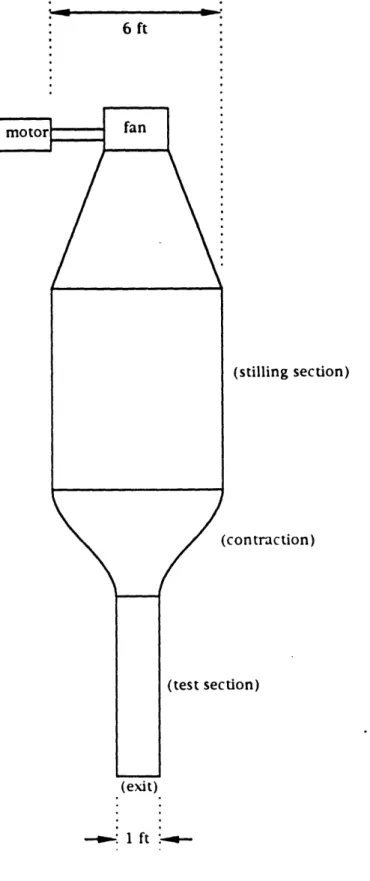
All experiments were performed in a 1 ft x 1 ft working section of a 6 ft x 6 ft

blowing type wind tunnel, illustrated in figure 4.1. The tunnel was powered by a 18.5 kW electric motor, producing a maximum wind speed of 50 ms- 1 at the entry to

the working section. This section was constructed out of plywood with the exception of one perspex face which allowed viewing of the experiments. The test section was calibrated for non-uniformities in the flow using a hot wire. The regions tested were those where the experiment's measurements were to be taken. The results are shown

6ft (stilling section) (con traction) (test section) (exit) -~ 1 ft:

4.2

Sources of Vorticity

4.2.1

The Vortex Tube

This device was constructed so that the mass flow rate and angle of swirl of the vortex flow entering the free stream could be controlled. The tube combined two air mass

flows, each tapped separately from a 25 kPag (150 psig) pressure line. The flows

entered the tube, one axially and the other tangentially. This is illustrated in the

drawing in figure 4.3. By independently throttling each mass flow rate, the nature of the vortical flow entering the generator could be varied.

The generator was constructed from aluminum, sealed, and streamlined using

plasticine. It was suspended in the tunnel by external supports. The tunnel blockage caused by the tube was 3%. A smoke hole was machined so that smoke could be injected into the cavity along with the axial air mass flow.

4.2.2

Wings

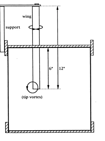
Two wings were used - one was a high aspect ratio (AR = 6) rectangular wing; the other a low aspect ratio (AR = 2.31) triangular wing. Both had a span of 12 inches.

The High Aspect Ratio Wing

The rectangular wing, constructed from wood and coated for smoothness, conformed to the NACA 0012 profile. It was mounted vertically as a half wing in the tunnel

and fixed by external supports. Its angle to the flow was determined by precalibrated

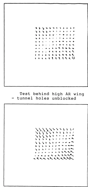
markings on the supports. The setup is shown in figure 4.4(a). The wing was used at speeds ranging from 5ms- 1to 25ms-' corresponding to Re, of - 18000 to - 90000,

Test behind low AR wing

- tunnel holes unblocked

ft. it

I rC

' '~

Test behind low AR wing

- tunnel holes blocked

Test behind high AR wing

- tunnel holes unblocked

Test behind high AR wing

- tunnel holes blocked Figure 4-2: Wind tunnel calibration

5mm = lm/s ~·\\1$ ~·~·,lT~4. *ftft 'a~ '1l** ·. ** 4.,~ 41% I ftt~ ft I ft S U ~

swirl mass flow

_int

I

I

I

I

I

I

I

I

t

and angles a = 40, 80, 100 and 150.

The Low Aspect Ratio Wing

The delta wing was cut from a -L" thick sheet of stainless steel. It was constructed as a half wing with no camber. The leading and trailing edges were machined sharp

(450 bevel) . The wing was mounted horizontally on the tunnel wall, and its angle of attack determined by precalibrated markings on the tunnel wall. The setup is shown in figure 4.4(b). This wing was used at wind speeds ranging from 5ms- 1 to 25ms- 1

corresponding to Rec of - 92000 to - 460000, and at a = 20, 40, 8' and 200.

4.3

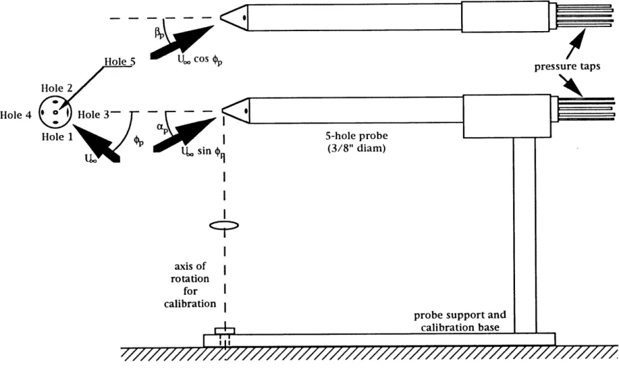
5-hole Pitot Probe

4.3.1

Description

This is a pressure measurement device that enables the user to determine the speed and direction of the flow in which it is placed. The probe used in the experiments

in this thesis was " in diameter with a conical tip having an apex angle of 600. It was manufactured by Dwyer [23]. The probe had one pressure tap at the apex of

the cone, and four pressure taps equally spaced circumferentially near the base of the cone, at a pitch circle diameter of .". The probe is shown in figure 4.5.

The advantage of using this type of probe was that it was simple, requiring little

equipment to support its operation. It was particularly useful since the measurement

of the flows' fluctuating components were not of interest. The disadvantage of the probe was related to its size. The factors affected were the locality of the

wing support 6"

r

...

(~TTTT

(a) Rectangular Wing (b) Delta Wing

Figure 4.4 - Wing geometry in tunnel working section

(vortex)

SDelta

the measurements due to static pressure gradients. The frontal area was 0.1% of the tunnel cross-sectional area, and 3.5% of the vortex tube exit area.

4.3.2

Probe Calibration

The geometry of the calibration setup was such that the apex of the conical tip remained spatially fixed throughout the calibration. This is shown in figure 4.5. The flow angles at the tip location were known through previous calibration of the wind tunnel. A pitot-static tube was used to measure the local flow speed. The pressures tapped from each of the five holes were measured as the probe was passed through a number of predetermined orientations. These orientations were measured by the probe roll angle, Op, and by the probe angle of incidence, p,. These would in turn determine the pitch and yaw angles (ca and #p) of the flow to the probe, as illustrated in figure 4.5, and which are calculated by the following formulae :

tan a = _{tan -y, sin ,p}

tan 3 = tan ,p cos p, (4.1)

Three nondimensional variables were introduced to describe the pressure mea-surements. These were denoted Ka, KO and Kq. which respectively represented the

pressures due to pitch and yaw, and the dynamic pressure as measured by the probe. The governing formulae were as follows :

q

P

Pi

+

P

+ P

+ P

P3 - P4

pressure taps

iX

I

I

probe support and calibration base

.0 . .0 0ý ý .ýý 0

. .0

.0,

.0

0 .1

/

Figure 4.5 - 5-hole pitot probe geometry Hole 4

for

-10-1000-.

"*--

I

Kq. = -- (4.2)

q

where Pi are the pressures at the holes as labeled in figure 4.5, i = 1 ... 5; and q is the dynamic pressure of the local flow (during the calibration this was measured using a pitot-static tube).

For each roll angle of the probe, then, K.' was curve fitted and found as a function of Cp, and similarly KO was found as a function of Pp . Thus

Kc, = Kcr(ap, Op)

with tan _P- = ~" _tan " from equation 4.1.

3p

These functions IK and KI were not simply expressible as functions K,(ap) and

Kp(/3p). It was instead necessary to produce a chart showing isoclines having values KI, and Kp . This chart is attached in Appendix A. This chart was valid only in the region of calibration, 17pl < 600. Similarly, for each roll angle, Kq. was curve fitted as a function of -, , thus Kq. = Kq.(Qy, Op), with

tan2 _{,p = tan}2 _{ac + tan}2 _,P

Such a fit yielded

Kq.(Q,, OP) = Co(Op) + Cl(Op)Y2 _{+ C}

2 (Op)Y4

with

Co(op) = 0.848 + 0.027€p

C2(qp) = -0.0929 + 0.065,p (4.3)

Again this fit was valid only for

[-,y

calibra-tion arose near -p = 460 - 530 where q* approached zero due to the probe geometry.

When this occurred, Ka and Kp took on infinite values, by their definitions in

equa-tion 4.2. In this region, however, a, and p, were quite insensitive to such large changes in K, and Ko so that this phenomenon did not present a problem.

4.3.3

Use of Calibrated Probe

The probe was placed in the flow field, with its tip at the point of measurement. The alignment of the probe set the orientation of the axis of measurement. For all the

experiments detailed herein, the probe was aligned with the free stream flow, and was held at zero roll angle (Op = 0).

The pressures from each of the five pressure holes were measured and used to calculate Ia , Ko and q* as defined in equation 4.2. By applying the chart in

Appendix A, Ka and Kf were used to find ap and p,, and hence also ,p and y,. Kq. followed from equation 4.2 and hence also the local flow speed, v, by using

4.4

Constant Temperature Crossed Hot Wire

Anemome-ter

4.4.1

Description, and Theory of Operation

The basic hot wire anemometer is made up of two parts : the hot wire probe and the compensating circuit. The hot wire probe has a thin cylindrical filament wire mounted between the tips of two conductive prongs. When a voltage is applied across the prongs, the wire is heated ohmically, and reaches a steady state temperature when the rate of heat transferred from the wire to the surrounding air balances the electrical power applied to heating the wire. As the speed of the air around the wire is increased, the rate of heat transfer through convection increases. Thus also the electrical power applied to the wire must be increased in order to keep the wire at a constant temperature. Since the power supplied to the wire changes with the electrical voltage applied across the prongs, thus this voltage is a measure of the flow speed. The control and measurement of this voltage is the purpose of the compensating circuit.

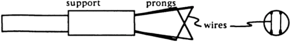
The hot wire anemometer is used to measure the component of flow normal to the wire. A single hot wire is able to determine only magnitude of the flow velocity, and not its direction. Other hot wire configurations allow measurement of flow direction. The crossed hot wire consists of two hot wire configurations mounted in parallel planes, but at 600 - 900 to each other when viewed normal to these planes. This is illustrated in figure 4.6. This configuration allows flow speeds and angles to be measured in the plane parallel to the wires. Other probes are available for simultaneous multi-component measurement.

The size of the filament varies for different applications. Those used for the experiments here were 51im in diameter, 5mm in length, and made of tungsten.

Com-monly the filament size is even smaller (2/m diameter, 2mm long) allowing for more local less intrusive measurement and faster frequency response to fluctuations in the flow velocity (since there is a smaller thermal mass to heat or cool). These are three advantages of using the hot wire probe over the pitot probe. Another is that the hot wire anemometer is much less sensitive to pressure gradients in the flow field. There are two distinct disadvantages of using a hot wire anemometer. One is that it needs to be recalibrated every time it is used. The other is its fragility which makes it more difficult to handle.

4.4.2

Calibration and Use

The calibration geometry for the crossed hot wire (X-wire) was identical to that used for the 5-hole pitot probe (see section 4.3.2). The probe was used at only two roll orientations : = 00 and 0 = 900, corresponding to flow occurring in the plane of the wires, and to flow occurring normal to the plane of the wires, respectively. For the calibration the X-wire was passed through yaw angles from -25' to +250 to the freestream direction. For each angle the voltages from the compensators for each of the two wires were recorded. This was done for a number of freestream velocities. Spline fits were then applied to the '0 = 00' calibration data. This spline fit procedure was rather complicated, and is explained in greater detail by Lueptow et. al. [21].

support pron

I__

wires

side view end view

The fit enabled the velocity and angle (in the plane of the wires) to be determined, given the voltages across the two wires. The '0 = 900' data was then used to correct these results. This correction was needed because a flow component normal to the plane of the wires altered the flow and heat transfer characteristics near the two wires.

Thus for each point of measurement data was recorded from the X-wire placed in two roll orientations : 0 = 00 and 0 = 900. For each orientation the flow velocity component was determined, then used to cross-correct the other component. The two results were then combined to get the overall flow velocity. A computer program was written by the author to perform the above-mentioned calculations. The listing is attached in Appendix B.

Chapter 5

The Vortex Tube

Vortex tubes have been used by other experimentalists for the study of breakdown [17, 18, 20]. The tube used in these experiments was most similar to that used by

Escudier et al [20]. The primary difference lay in the use of the vortex developed in the tube. Escudier et al performed all their experiments within the tube, whereas here the studied vortex was expelled from the tube into the free stream.

The vortex tube was designed so that flow conditions at the exit of the generator

were not changing with axial distance. In order for these conditions to remain as the vortex entered into the free stream, it was necessary to impose a condition on the flow. This condition required the pressure on each side of the vortex/free stream interface to match. It was postulated that this condition could be physically observed by using smoke visualization. Smoke injected into the generator's cavity would exit and remain

in a cylindrical region downstream of the exit if this condition held true. Otherwise the smoke envelope would diverge or converge. The graph in figure 5.1, obtained

experimentally, shows axial and swirl mass flows (rh, and rh,) that could be used to satisfy this observed condition given a free stream velocity.

to

6

Figure 5-1: Conditions for parallel smoke flow

Several points on this graph were arbitrarily chosen, and measurements were taken using the 5-hole probe. These measurements were for rhia = 2.67 liters/min, and rh, = 5.34 liters/min at 1, 2 and 5 exit diameters downstream of the tube. The results of these are shown in figure 5.2. In all these cases, a strong inflow is evident. Also axial velocity defects and static pressure defects exist in the cores, and the vortices decay rapidly in the downstream direction.

The observation of the high inward radial velocity components raised questions as to whether there were factors affecting the operation of the 5-hole probe. One factor was a radial static pressure gradient. The probe was calibrated to measure a dynamic pressure and would interpret any imposed static pressure gradient as a dynamic pressure in the opposite direction to the gradient. A second factor was the effect of the probe blockage on the flow direction. A blockage placed in a shear flow causes the flow to alter its direction near the blockage. The characteristics of the flow measurements indicated that both of these factors would cause the flow to appear to have an inward radial velocity component.

For one set of flow conditions, the 5-hole probe results were compared to the those obtained by using a hot wire anemometer. The results of these measurements are shown in figure 5.3. It was surprising to note that the hot wire results were very similar to the results of the 5-hole probe. The factors affecting the 5-hole probe were thus deemed insignificant. It was decided instead that the method for observing pressure-matching at the tube exit had been incorrect. The cylindrical smoke surface exiting the tube contained not only the vortex, but also the turbulence which was shed at the tube exit. Thus the cylindrical surface did not indicate the vortex was neither growing nor decaying.

Hot wire measurements were taken for the two other flow conditions. These conditions were for rha = 10.68 liters/min, and rih, = 8.01 liters/min at 2 and 5 exit diameters downstream of the tube. The results are shown in figure 5.4.

1 exit diameter downstream 2 exit diameters downstream 3 exit diameters downstream

Figure 5-2: 5-hole pitot probe results

m, =2.67 i/min; m, =5.34 1/min

U. =5 m/s

1 exit diameter downstream

Figure 5-2: 5-hole pitot probe results

r~ =2.67 l'/min; m, =5.34 1/min

U, =5 m/s

axial velocity plots

--- - ---- ---b q iI t S. . 0 h '. e

72

IT

It

I

7

I

0

tA

Figure 5-3: Hot wire results, radial inflow mi =2.67 1/min; i, =5.34 1/min

U. =5m/s

swirl velocity plots

Vortex Tube Uu 5m/ s ; z/D a 1

axial m a 2.67 1/min ; swirl m = 5.34 i/min

2 4 6 I 8I

Vortex Tube

U a Sm/s ; /D . 2

axial m a 2.67 i/min ; swirl m a S.34 k/min

0 2 4 6 8 10 12

Fieure 5.3: Hot wire results. radial inflow

X traverse # * traverse #2 M traverse #3 + traverse #4 traverse #5 0 traverse #6 traverse #7 Straverse #8 traverse #9 (* 3/13 in) traverse position traverse #1 I traverse #2 traverse #3 traverse #4 traverse #5 traverse #6 traverse #7 traverse #8 traverse #9 _ '

Ed -It L -exit dian A~'

p~77

1

'7

7

2

a

5 exit diameters downstream Figure 5-4: Hot wire results, no radial inflow

m. =10.68 1/min; rh, =8.01 1/min

U,,=5 m/s

swirl velocity plots

2

Z_

Vortn Tube

U • 5m11; liD. 2

axial m • 10.611 IImln; Iwlrl m • ..01 IImin

.

..

•

•

•

Iraverse pOlillon (. 3/13 In)

10 12

Vorlu Tube U • 5m1s Z/D .. 5

axial m • 10.68 11m i n ; Iwirl m • 8.01 IImin

•

..

_•

!

_•

...

_..

··

Ira vern (* 3/13 In)

10 12

Fi{!ure 5.4: Hot wire resultsl no radial inflow

Figure 5.4(a) shows the vortex to have no inward radial velocity component. However, an axial velocity defect and rapid decay of the vortex are still evident. The observation of an axial defect was expected: Escudier et alwere not able to achieve axial velocity excesses in their vortex tube experiments without considerable tube exit

area contraction. This attribute was not of importance since the final goal was to use the vortex in breakdown experiments and VBD is always preceeded by a falling off of the centerline axial velocity to zero. The observation of the rapid decay, however, meant the vortex would not be observable (and hence useful) at considerable distances ( > 5 - 10 exit diameters) downstream of the tube.

The reason for the rapid decay was, it was concluded, that although the vortex within the tube was strong and well developed, the external flow field did not have the pressure field necessary to sustain the vortex. The case of the vortex tube was

unlike the case of a wing, for example, where the wing imposes a pressure field to

create and thereby also sustain the vorticity. Experiments using the vortex tube were discontinued, since the physical phenomena differed from that behind a lifting wing.

Chapter 6

The High and Low Aspect Ratio

Wings

6.1

Method of Data Analysis

The analysis of the raw hot wire data required two steps. The first was the conversion of the hot wire voltage readings into the velocity components (see section 4.4.2). The second was a processing of the velocity data to fit a theoretical model of the vortices shed from a high AR wing. The results derived in chapter 3 were used for the sec-ond step. Equation 3.12 was rewritten by introducing an effective radius, r,, such that

v

K

with r+ h)((b - )2 + h2_{) (6.1)}

This defined a relationship similar to that for a single line vortex, between the velocity I VI and an effective radius, r,.

For any data point, the crossplane velocity, V, was separated into its polar components, ImV, and € (see figure 6.1). To apply the model described above, the component of velocity in the direction prescribed by the model was found by

YVI = IVyI

cos(C

- 0)

(6.2)

Thus to find the tip vortex circulation one used equations 6.1 and 6.2.

A straight line fit of JIY against 1- in the irrotational flow field was performed. The gradient of this line yielded K and was thus proportional to the value of the circulation, F = 2irK.

An alternate method for finding the circulation was by numerically integrating the velocity field over a closed contour path which passed through only the region of potential (irrotational) flow, and which enclosed the vortex center (figure 6.2). This integral, by definition, was equal to the circulation:

P = yV ds

The reduced data are presented in the plots attached as Appendices C to K. They show velocity field plots, graphs of azimuthal and axial velocities, and contours of streamlines and axial velocities, for each wing and flow condition. The traverse geometries are shown in figure 6.3.

of measurement I I,

I

T...

(Wing trailing edge)

V

467 M

Enlargement of circled region

1 2 25 26 High aspect ratio (rectangular) wing

traverse geometry

1 (15) 35

Low aspect ratio (delta) wing measurement volume

Figure 6.2 - Paths of integration for calculation of circulation

-.- path of integration

wing

12... -~--- traverse position -~ 25 26 wing

_--

-r

....

avers

#3

_7

_

_J-1

Low aspect ratio (delta) wing

measurement volume

Figure 6.3 - Traverse geometries t

taverse #L

-(tip

vortex)---t

High aspect ratio (rectangular) wing

---

----

---

---

I

w---wing

--1 2

...

6.2

General results

6.2.1

Circulation

The values of circulation, calculated by the line integral method, are shown in table 6.1. They are compared with the expected values of circulation, calculated based on a and on previously collected data [22]. The values of circulation, calculated by curve fitting the data, are not shown, except in the cases of the low AR wing at a = 200 where the contours for the line integrals passed through the viscous regions of the vortex flow fields (see figure 6.2 and appendix C).

The azimuthal velocity results (appendices D and H) show graphs of those veloc-ities normalized as per equations 3.16 and 3.17 . The circulations used to normalize the velocities are those calculated by the line integral method. This choice allows comparison of the circulations calculated by the two methods. For the results to compare well, a line of unit gradient would fit the data points closely. The plots show that this is indeed the case, with the exception of the cases of the low AR wing at

High AR Wing Low AR Wing Table 6.1

Uoo

0.02 0.04 0.08 0.02 0.04 0.08 0.02 0.04 0.08 0.02 0.04 0.08 0.20 0.02 0.04 0.08 0.20 0.02 0.04 0.08 0.20

ri

(0.2015)

N/A

N/A

N/A

This method of comparison was chosen because, in most cases, the line that

most suitably fit the data were not those indicated by least squares fits. Rather, the

points could only be fitted by visual interpolation, subject to the associated errors.

Although the calculated circulations do not match well to those expected, they

are consistent across the range of freestream velocities at each angle. Table 6.1

One anomaly of the azimuthal velocity plots is that the line fits do not always

pass through the origin. In essence, this would imply that the velocity in the far field did not decay to zero. Aside from the inherent experimental error, there are two

sources that might have contributed to the phenomenon. They are the curvature of

the vortex line, and the extent to which the vortex has rolled up. Those and other sources of error are discussed in section 6.3.

6.2.2

Axial Velocity Profiles

In the results for the low AR wing the axial velocity profiles show a defect in the core region, although near the edge of the core the profiles sometimes show a slight

excess. The magnitude of the maximum excesses and defects are shown in table 6.2.

The results for the high AR wing below a = 15' are the same. One set of results for this wing at a = 100 aoa was measured at 2 = 1, 2 and 5. The circulations for these data were F = 0.0504, 0.0370 and 0.0473 respectively, using the closed contour

integral method. These data are of interest because they show velocity excesses in the cores for f = 1, and 2. These are shown in figure 6.4 and in table 6.2.

Rectangular Wing (AR=6)

U Sm/s ; 100 sea

s/c 1

1.05

--10 0 10

Rectangular Wing (AR=6)

U a Sm/s ; 100 SOa z/c a 2

0.95

-0.85

0.75 *

Figure 6.4: High AR wing at 100 - Axial velocity profiles

X traverse #1 Staverse #2 0 trvere #3 + traverse #4 Straverse #5 Stravase #6 & traverse #7

traverse position (* 4/13 in)

X traverse #1 0 travcrse #3 Straverse #4 - traverse #5 c traverse #6 0 traverse #7 traverse #8 Straverse #9 W traverse # 11 (* 4/13 in) traverse position 1 r I I

-W

Rectangular Wing

Delta Wing

Table 6.2

Uoo a (degrees) % Velocity Defect

15.0 30.0 35.0 10.0 2.5 36.0 2.0 6.0 36.0 2.5 10.0 24.5 58.0 7.0 12.5 30.0 56.5 9.0 12.0 29.0 52.0 % Velocity Excess 1.0 2.0 1.0 1.0 2.5 2.0 1.5 4.5 0.5 1.6 1.8 2.0 3.9 5.5 0.7 2.2 3.0 0.2 2.9 1.4 2.5

In the other cases, the velocity excesses are disregarded since they are small and mostly lie within experimental error. It should be noted that the velocity minima in the cores do not correspond to the physical velocity minima. This results from the

contribution of the wakes behind the wing.

The maximum velocity defects for the rectangular wing are inaccurate due to

_1

--- ---

~-I

I

the small core sizes of the tip vortices. The core sizes are of the same order, if not smaller than, the measurement grid resolution of 4 mm. This is shown in table 6.3.

Table 6.3 U. a (degrees) 5 2 5 4 5 8 5 15 5 20 15 2 15 4 15 8 15 15 15 20 25 2 25 4 25 8 25 15 25 20

Core Size (# grid spacings) Low Aspect Ratio High Aspect Ratio

3.5 3.5 0.6 3.0 0.9 - _2.2 6.0 2.5 3.0 0.8 3.0 1.3 - _2.2 6.0 2.0 3.0 0.8 3.0 1.3 - _1.9 7.5

6.2.3

The Wake

The wakes are apparent in the axial velocity graphs for both wings except in the

cases of the low AR wing at a = 8' and 200 due to the limited extent of the region

of measurement. The wakes are also seen in the contour plots (Appendices E and

I). Their positions below the vortex core centers are estimated from the graphs. The

The percentage velocity defects in the wakes below both wings are also estimated and found to be around 5% - 8% of the free stream velocity. They appear unrelated to the conditions, and are, in any case, subject to measurement and experimental errors.

It is seen that the wakes behind both wings move away from the cores with

down-stream distance, more so for the low AR wing. The reason lies in that the vorticity in the wake is primarily transverse vorticity, whilst that in the induced vortex is pri-marily streamwise vorticity. Thus they convect differently in the freestream. The

vertical velocity of the transverse vortex depends on the intensity of the vortex. Flow around an unstalled high AR wing is such that this vorticity is low. The vorticity is

high when there is flow separation from the trailing edge of the wing.

This is the case for a low AR wing, except at small a. The results in table 6.4 demonstrate this wake phenomenon well. Only in the cases of the low AR wing at a = 4' are the positions of the wake greatly different from the other cases.

6.2.4

Vortex Core Positions

Chapter 2 reviewed the findings of Spreiter and Sachs [9] dealing with the motion of vortex cores away from wing trailing edges. Those findings are used as a basis for comparison with the present results. Table 6.5 shows this comparison. From the velocity field plots (Appendix C) the core centers were located by finding the inter-section of the normals to the velocity vectors near the center. The lateral positions of the cores were normalized as

y - s' S - S

Table 6.4

Uo, a (degrees) % Defect yt.e. - y,,wake(mm)

High 5 4 4 0.369 AR 5 8 6 0.538 Wing 5 15 7 0.538 15 4 7 0.391 15 8 7 0.523 15 15 8 0.538 25 4 7 0.431 25 8 9 0.477 25 15 - 0.508 Low 5 2 4.1 0.462 AR 5 4 3.1 1.293 Wing 15 2 4.5 0.562 15 4 6.1 1.136 25 2 6.1 0.633 25 4 6.4 1.273

For the low AR wing, the height of the core centers above the wing trailing edge are not presented because they remain nearly constant for all the cases, except when a = 20, where the flow mechanism is different (see normalized version).

6.3

Measurement Errors

Three factors contributed to the measurement error. The first was that associated with the positioning of the hot wire and of the wings. The angles of attack of the wings were visually accurate (within 0.50) but did not affect the outcome of the experiment since the results were normalized using the measured circulation. Positioning of the hot wire affected mainly the results within the vortex core where the velocity gradients were high.

The equation that approximates the core and outer regions is,

r

f2

V

(6.3)

Table 6.5

Angle of Attack, a

High AR Wing Low AR Wing

40 80 150 20 40 80 200

Uo"= 5ms-' 0.642 0.688 0.479 0.540 0.186 0.028 0.112

Uo = 15ms-1 0.665 0.688 0.730 0.572 0.237 -0.028 0.044

Uo, = 25ms-' 0.674 0.660 0.805 0.563 0.233 -0.014 0.038 Spreiter and Sachs [9] 0.888 0.823 0.726 0.633 0.451 0.247 0.003 Kaden [10] 0.888 0.823 0.721 0.614 0.386 0.000 0.000

with fr = i being the nondimensional core radius. The smallest value of fi is near unity, so that

r

Thus the error e, is

Hence the above statement is confirmed.

If the positioning error is ~ 0.5 mm and since E ~ 0.5, thus

le 0.25 f (6.4)

0.25

2- fr > rc

A second factor in measuring error was the time-averaging of the hot wire signal, necessary due to the tunnel free stream fluctuations in the tunnel flow. This is a small effect most dominant in the potential flow region of the vortex. It appears as a voltage fluctuation of the hot wire reading, of the order of 0.01 volts. Vortex core wandering is a strong effect dominant in the core region. It appears as hot wire voltage fluctuations of the order of 0.10 volts. The following is an error analysis used to determine the error in the interpreted data.

The data sets for calibrating the X-wire probe were very similar. An example data set is plotted in figure 6.5. It shows the two voltages, E1 and E2, across the two wires. They are grouped into sets representing the probe at constant angle to the flow, and

Figure 6-5: Example of calibration data

placed in a constant flow velocity. For the purposes of this analysis, constant velocity

lines fitted to the data points are quadratic and constant angle lines are linear.

The approximating equation for axial velocity is

U

= a(E2 - kE

1

E

2

+

E2)

+

b(E2

- kE

E

2

+

E')

2

For IIAE1I|

_ 0.1; k 1.

IIAE

2

ll 2 I•AEll then

AU : (El - E2)(1 + 0.2(E2 - EIE2 +

E2))II|AE 1

The maximum error is

= 14%

The approximating equation for angle is

/_ 2 arctan(E)

-El

2

and using similar assumptions then

2(E

_{+ E}

E1+

E2

2.8210

A third factor results from the spline fit error. The method uses several steps

which involve interpolation of the calibration data. The associated errors are of

within O.lms- 1 and 10. Here for each data set and associated measurements, the

error is not random as are the cases of the two above mentioned errors. The error

is fixed throughout the set of measurements and this is likely to appear in the plots an offset. For example, in the plots of azimuthal velocity (Appendices D and H) this

6.4

Discussion

6.4.1

Circulation

The High AR Wing

The range of deviation of the points from the expected unit gradient line is outside

the range of error, if the points are viewed collectively. However, the data points of separate traverses lie parallel to the reference line. This seems to indicate that the circulation was estimated correctly, and that the quasi-2D assumption was accurate.

Table 6.6, calculated from the results of Spreiter and Sachs, shows the positions

downstream of the trailing edge where the vortices become rolled up.

Clearly, at 2 chordlengths downstream the high AR wing tip vortices are not rolled up. Yet it appears that the shape of the vortex was well estimated. That is to say the

rate at which the vortex diffused into a Burger's vortex was comparable to the rate

at which the vortex rolled up. Another observation is that the line fits are better at

the high velocities, whereas at 5ms- 1 a distinct non-linearity is seen (particularly for

I < 1). This is most likely a Reynolds number effect which affected diffusion during

roll-up. A higher Reynolds number accompanies more rapid diffusion. Table 6.6

Roll-up Distance,

-a (degrees) High AR Wing Low AR Wing

2 - 8.296

4 53.76 4.148

8 26.88 2.074

15 13.44

The results for the wing at a = 100 show that at 2 = 2 the circulation is lower than at 2 = 5. This is expected because the vortex is still rolling up. The result at 2 = 1 is not useful because the integration contour lies in the viscous core region. A summary

of circulations is shown in figure 6.6. With the exception of the two points at a = 40, at 15 ms- 1 and 25 ms-1, the data lie close to a line parallel to the theoretical estimate (obtained using the lift curve slope CL, = 27r). The intercept indicates a zero lift angle of attack of about -50. This is the combination of manufacturing error in the wing, and error in the angular positioning of the wing. Examination of the wing showed

that it was twisted by about 50 thereby justifying the first postulate. It might be noted that at a = 150 the twisted wing should be stalled, yet it does not seem to be

affecting the results in figure 6.6.

Low AR wing

The range of deviation of the points from the expected unit gradient line is again outside the range of error. Only at the higher speeds or angles of attack do points fit

closely to the line. The close fit at the higher a is in agreement with the results of table 6.6. Unlike the high AR wing, the vortex over a delta wing rolls up more rapidly,

whilst its vorticity diffusion occurs at the same rate , controlled by the Reynolds number. The appropriate vortex model at the station of measurement lies somewhere between the Hall and Burger models.

There are other sources of error. One is the changing of flow conditions with changing Reynolds number. Transition from laminar to turbulent flow occurs near

Rec - 10000. A second is that there may have been more than one method of vortex

generation taking place at the low angles of attack (20 and 40), particularly at a = 20.

Separation may not be have been occurring over the entire leading edge (if any part

of it at all). For this reason the data for the wing at a = 20 seems somewhat better