HAL Id: hal-02434232
https://hal.archives-ouvertes.fr/hal-02434232v2
Preprint submitted on 10 Jul 2020
HAL is a multi-disciplinary open access
archive for the deposit and dissemination of sci-entific research documents, whether they are pub-lished or not. The documents may come from teaching and research institutions in France or abroad, or from public or private research centers.
L’archive ouverte pluridisciplinaire HAL, est destinée au dépôt et à la diffusion de documents scientifiques de niveau recherche, publiés ou non, émanant des établissements d’enseignement et de recherche français ou étrangers, des laboratoires publics ou privés.
Stationary Heston model: Calibration and Pricing of
exotics using Product Recursive Quantization
Gilles Pagès, Thibaut Montes, Vincent Lemaire
To cite this version:
Gilles Pagès, Thibaut Montes, Vincent Lemaire. Stationary Heston model: Calibration and Pricing of exotics using Product Recursive Quantization. 2020. �hal-02434232v2�
Stationary Heston model: Calibration and Pricing of exotics
using Product Recursive Quantization
Vincent Lemaire ∗ Thibaut Montes ∗† Gilles Pagès ∗
July 10, 2020
Abstract
A major drawback of the Standard Heston model is that its implied volatility surface does not produce a steep enough smile when looking at short maturities. For that reason, we introduce the Stationary Heston model where we replace the deterministic initial condition of the volatility by its invariant measure and show, based on calibrated parameters, that this model produce a steeper smile for short maturities than the Standard Heston model. We also present numerical solution based on Product Recursive Quantization for the evaluation of exotic options (Bermudan and Barrier options).
Introduction
Originally introduced by Heston in [Hes93], the Heston model is a stochastic volatility model used in Quantitative Finance to model the joint dynamics of a stock and its volatility, denoted pStpxqqtě0
and pvtxqtě0, respectively, where v0x “ x is the initial condition of the volatility. Historically, the
initial condition of the volatility x is considered as deterministic and is calibrated in the market like the other parameters of the model. This model received an important attention among practitioners for two reasons: first, it is a stochastic volatility model, hence it introduces smile in the implied volatility surface as observed in the market, which is not the case of models with constant volatility and second, in its original form, we have access to a semi closed-form formula for the characteristic function which allows us to price European options (Call & Put) almost instantaneously using the Fast Fourier approach (Carr & Madan in [CM99]). Yet, a complaint often heard about the Heston model is that it fails to fit the implied volatility surface for short maturities because the model cannot produce a steep-enough smile for those maturities (see [Gat11]).
Noticing that the volatility process is ergodic with a unique invariant distribution ν “ Γpα, βq where the parameters α and β depend on the volatility diffusion parameters, it has been first proposed by Pagès & Panloup in [PP09] to directly consider that the process evolves under its stationary regime in place of starting it at time 0 from a deterministic value. We denote by pStpνqqtě0 and pvνtqtě0 the couple asset-volatility in the Stationary Heston model. Replacing
the initial condition of the volatility by the stationary measure does not modify the long-term behavior of the implied volatility surface but does inject more randomness into the volatility for short maturities. This tends to produce a steeper smile for short maturities, which is the kind of behavior we are looking for. Later, the short-time and long-time behavior of the implied volatility
∗
Sorbonne Université, Laboratoire de Probabilités, Statistique et Modélisation, LPSM, Campus Pierre et Marie Curie, case 158, 4 place Jussieu, F-75252 Paris Cedex 5, France.
†
generated by such model has been studied by Jacquier & Shi in [JS17]. Another extension of the Heston model have been suggested and extensivel analyzed in order to reproduce the slope of the skew for short-term expiring options: the Rough Heston model where the volatility satisfies a Voltera equation driven by a "rough" Liouville process with H-Hölder paths, H “ 0.1 (see [JR16, GJRS18, GJR18, CGP18, GR19] for details on the model and numerical solutions).
An other extension of the Heston model have been suggested in order to be able to reproduce the slope of the skew for short-term expiring options: the Rough Heston model (see [JR16, GJRS18, GJR18, CGP18, GR19] for details on the model and numerical solutions).
In the beginning of the paper, we briefly recall the well-known methodology used for the pricing of European option in the Standard Heston model. Based on that, we express the price I0 of a European option on the asset STpνq as
I0“E“ e´rT ϕpSTpνqq
‰
“E“fpv0νq
‰
(0.1)
where f pvq is the price of the European option in the Standard Heston model for a given set of parameters. The last expectation can be computed efficiently using quadrature formulas either based on optimal quantization of the Gamma distribution or on Laguerre polynomials.
Once we are able to price European options, we can think of calibrating our model to market data. Indeed the parameters of the model are calibrated using the implied volatility surface observed in the market. However, the calibration of the Standard Heston model is highly de-pending on the initial guess we choose in the minimization problem. This is due to an over-parametrization of the model (see [GR09]). Hence, when we consider the Heston model in its stationary regime, there is one parameter less to calibrate as the initial value of the volatility is no longer deterministic. The stationary model tends to be more robust when it comes to calibration.
In the second part of paper, we deal with the pricing of Exotic options such as Bermudan and Barrier options. We propose a method based on hybrid product recursive quantization. The "hybrid" term comes from the fact that we use two different types of schemes for the discretization of the volatility and the asset (Milstein and Euler-Maruyama). Recursive quantization was first introduced by Pagès & Sagna in [PS15]. It is a Markovian quantization (see [PPP04]) drastically improved by the introduction of fast deterministic optimization procedure of the quantization grids and the transition weights. This optimization allows them to drastically reduce the time complexity by an order of magnitude and build such trees in a few seconds. Originally devised for Euler-Maruyama scheme of one dimensional Brownian diffusion, it has been extended to one-dimensional higher-order schemes by [MRKP18] and to medium dimensions using product quantization (see [FSP18, RMKP17, CFG18, CFG17, PS18]). Then, once the quantization tree is built, we proceed by a backward induction using the Backward Dynamic Programming Principle for the price of Bermudan options and using the methodology detailed in [Sag10, Pag18] based on the conditional law of the Brownian Bridge for the price of Barrier options.
The paper is organized as follows. First, in Section 1, we recall the definition of the Standard Heston model and the interesting features of the volatility diffusion which bring us to define the Stationary Heston model. In Section 2, we give a fast solution for the pricing of European options in the Stationary Heston model when there exists methods for the Standard model. Finally, once we are able to price European options, we can define the optimization problem of calibration on implied volatility surface. We perform the calibration of both models and compare their induced smile for short maturities options. Once this model has been calibrated, in Section 3, we propose a numerical method based on hybrid product recursive quantization for the pricing of exotic financial products: Bermudan and Barrier options. For this method, we give an estimate of the L2-error introduced by the approximation.
1
The Heston Model
The Standard Heston model is a two-dimensional diffusion process pStpxq, vxtq solution to the Stochastic Differential Equation
$ ’ ’ & ’ ’ % dStpxq Stpxq “ pr ´ qqdt ` a vx t`ρdĂWt` a 1 ´ ρ2dW t ˘ dvtx“ κpθ ´ vtxqdt ` ξavtxdĂWt (1.1) where
• Stpxq is the dynamic of the risky asset, • vx
t is the dynamic of the volatility process,
• S0pxq “ s0 ě 0 is the initial value of the process,
• r P R denotes the interest rate, • q P R is the dividend rate,
• ρ P r´1, 1s is the correlation between the asset and the volatility, • pW, ĂW q is a two-dimensional standard Brownian motion,
• θ ě 0 the long run average price variance, • κ ě 0 the rate at which vx
t reverts to θ,
• ξ ě 0 is the volatility of the volatility, • vx
0 “ x ě 0 is the deterministic initial condition of the volatility.
This model is widely used by practitioner for various reasons. One is that it leads to semi-closed forms for vanilla options based on a fast Fourier transform. The other is that it represents well the observed mid and long-term market behavior of the implied volatility surface observed on the market. However, it fails producing or even fitting to the smile observed for short-term maturities.
Remark 1.1 (The volatility). One can notice that the volatility process is autonomous thence we are facing a one dimensional problem. Moreover, the volatility process is following a Cox-Ingersoll-Ross (CIR) diffusion also known as the square root diffusion. Existence and uniqueness of a strong solution to this stochastic differential equation has been first shown in [IW81], if x ě 0. Moreover, it has been shown, see [LL11], that if the Feller condition holds, namely ξ2 ď 2κθ, for every x ą 0, then the unique solution pvxtqtě0 satisfies
@t ě 0, Ppτ0x“ `8q “ 1 (1.2)
where τ0x is the first hitting time defined by
τ0x “ inftt ě 0 | vxt “ 0u where inf H “ `8. (1.3)
Moreover, the CIR diffusion admits, as a Markov process, a unique stationary regime, charac-terized by its invariant distribution
ν “ Γpα, βq (1.4)
where
Based on the above remarks, the idea is to precisely consider the volatility process under its stationary regime, i.e., replacing the deterministic initial condition from the Standard Heston model by a ν-distributed random variable independent of pW, ĂW q. We will refer to this model as the Stationary Heston model. Our first aim is to inject more randomness for short maturities (t small) into the volatility but also to reduce the number of free parameters to stabilize and robustify the calibration of the Heston model which is commonly known to be overparametrized (see e.g. [GR09]).
This model was first introduced by [PP09] (see also [IW81], p. 221). More recently, [JS17] studied its small-time and large-time behaviors of the implied volatility. The dynamic of the asset price pStpνqqtě0 and its stochastic volatility pvtνqtě0 in the Stationary Heston model are given by
$ ’ ’ & ’ ’ % dStpνq Stpνq “ pr ´ qqdt ` a vνt`ρdĂWt` a 1 ´ ρ2dW t ˘ dvtν “ κpθ ´ vtνqdt ` ξ a vν tdĂWt (1.6) where vν 0 „ Lpνq „ Γpα, βq with β “ 2κ{ξ2, α “ θβ. S pνq
0 , r and q are the same parameters as
those defined in (1.1) and the parameters ρ, θ, κ, θ and ξ can be described as in the Standard Heston model.
2
Pricing of European Options and Calibration
In this section, we first calibrate both Stationary and Standard Heston models and then compare their short-term behaviors of their resulting implied volatility surfaces. For that purpose we relied on a dataset of options price on the Euro Stoxx 50 observed the 26th of September 2019 (see Figure 1). This is why, as a preliminary step we briefly recall the well-known methodology for the evaluation of European Call and Put in the Standard Heston model. Based on that, we outline how to price these options in the Stationary Heston model. Then, we describe the methodology employed for the calibration of both models: the Stationary Heston model (1.6) and the Standard Heston model (1.1) and then we discuss the obtained parameters and compare their short-term behaviors.
2.1 European options
The price of the European option with payoff ϕ on the asset STpνq, under the Stationary Heston model, exercisable at time T is given by
I0 “E“ e´rT ϕpSTpνqq‰. (2.1)
After preconditioning by v0ν, we have
I0 “E ” E“ e´rTϕpSTpνqq | σpv0νq‰ ı “E“fpvν0q ‰ (2.2)
where f pvq is the price of the European option in the Standard Heston model with deterministic initial conditions for the set of parameters λpvq “ ps0, r, q, θ, κ, ξ, ρ, vq.
Example 2.1 (Call). If ϕ is the payoff of a Call option then f is simply the price given by Fourier transform in the Standard Heston model of the European Call Option. The price at time
0, for a spot price s0, of an European Call Cpλpvq, K, T q with expiry T and strike K under the
Standard Heston model with parameters λpvq “ ps0, r, q, θ, κ, ξ, ρ, vq is
Cpλpvq, K, T q “ E“ e´rTpSTpvq´ Kq` ‰ “ e´rT ´ E“STpvq1STpvqěK ‰ ´ KE“ 1Spvq T ěK ‰¯ “ s0e´qT P1`λpvq, K, T ˘ ´ K e´rTP2`λpvq, K, T ˘ (2.3)
with P1`λpvq, K, T ˘ and P2`λpvq, K, T ˘ given by
P1`λpvq, K, T ˘ “ 1 2 ` 1 π ż`8 0 Reˆ e ´iu logpKq iu ψ`λpvq, u ´ i, T ˘ s0epr´qqT ˙ du P2`λpvq, K, T ˘ “ 1 2 ` 1 π ż`8 0 Reˆ e ´iu logpKq iu ψ`λpvq, u, T ˘ ˙ du (2.4)
where i is the imaginary unit s.t. i2 “ ´1, ψ`λpvq, u, T ˘ is the characteristic function of the logarithm of the stock price process at time T . Several representations of the characteristic func-tion exist, we choose to use the one proposed by [SST04, Gat11, AMST07], which is numerically more stable. It reads
ψ`λpvq, u, T ˘ “ E “ eiu logpSpvqT q| Spvq 0 , x ‰ “ eiuplogps0q`pr´qqT q ˆ eθκξ´2 ` pκ´ρξui´dqT ´2 logpp1´g e´dtq{p1´gqq˘ ˆ ev2ξ´2pκ´ρξui´dqp1´e´dtq{p1´g e´dtq (2.5) with
d “apρξui ´ κq2´ ξ2p´ui ´ u2q and g “ pκ ´ ρξui ´ dq{pκ ´ ρξui ` dq. (2.6)
Hence, in (2.2), f pvq can be replaced by C`λpvq, K, T ˘, which yields I0 “E“ e´rTpSTpνq´ Kq` ‰ “E ” C`λpvν 0q, K, T ˘ı . (2.7)
Now, we come to the pricing of European options in the Stationary Heston model, using the expression of the density of vν0 „ Γpα, βq, (2.2) reads
I0 “E“fpvν0q ‰ “ ż`8 0 f pvq β α Γpαqv α´1e´βvdv. (2.8)
Now, several approaches exists in order to approximate this integral on the positive real line.
• Quantization based quadrature formulas. One could use a quantization-based cubature formula with an optimal quantizer of vν0 with the methodology detailed in Appendix D. Given that optimal quantizer of size N , pvN0 , we approximate I0 by pI0N
p I0N “E“fppv0Nq‰“ N ÿ i“1 f pv0,iNqP`vp N 0 “ vN0,i˘. (2.9)
Remarks 2.2. In one dimension, the minimization problem, that consists in building an optimal quantizer, is invariant by linear transformation. Hence applying a linear transformation to an optimal quantizer preserves its optimality. For example, if we consider an optimal quantization
p
XN of a standard normal distribution N p0, 1q then µ ` σ pXN is an optimal quantizer of a normal distribution N pµ, σ2q and the associated probabilities of each Voronoï centroid stay the same. In our case, noticing that if we consider a Gamma random variable X „ Γpα, 1q then the rescaling of X by 1{β yields X{β „ Γpα, βq. Hence, for building the optimal quantizer pv
N
0 of v0ν, we can
build an optimal quantizer of X „ Γpα, 1q and then rescale it by 1{β, yielding pv
N
0 “ pXN{β. Our
numerical tests showed that it is numerically more stable to use this approach.
In order to build the optimal quantizer, we use Lloyd’s method detailed in Appendix D to X „ Γpα, 1q with the cumulative distribution function FXpxq “PpX ď xq and the partial first moment KXpxq “ErX 1Xďxs given by
@x ą 0, FXpxq “ 1 Γpαqγpα, xq, KXpxq “ αFXpxq ´ xαe´x Γpαq , otherwise, FXpxq “ 0, KXpxq “ 0, (2.10)
where γpα, xq “ şx0tα´1e´tdt is the lower gamma function. And the associated probabilities of
the optimal quantizervp0N are given by (D.10)
P`pv N 0 “ v0,iN ˘ “P`XpN “ xNi ˘ “ FX`x N i`1{2 ˘ ´ FX`x N i´1{2 ˘ (2.11) where @i PJ2, N K, xNi´1{2 “ x N i´1`xNi 2 and x N 1{2“ 0 and x N N `1{2“ `8.
• Quadrature formula from Laguerre polynomials. One could also use an algorithm based on fixed point quadratures for the numerical integration. Indeed, noticing that the density we are integrating against is a gamma density which is exactly the Laguerre weighting function (up to a rescaling). Then, I0 rewrites
I0“ ż`8 0 f pvq β α Γpαqv α´1e´βvdv “ β α Γpαq ż`8 0 f pvqωpvqdv (2.12)
where ωpvq “ vα´1e´βv is the Laguerre weighting function. Then, for a fixed integer n ě 11, I 0 is approximated by r I0n“ β α Γpαq n ÿ i“1 ωif pviq (2.13)
where the ωi’s are the Laguerre weights and the vi’s are the associated Laguerre nodes.
2.2 Calibration
Now that we are able to compute the price of European options, we define the problem of minimization we wish to optimize in order to calibrate our models parameters. Let PSH be the set of parameters of the Stationary Heston model that needs to be calibrated, defined by
PSH “ pθ, κ, ξ, ρq PR`ˆR`ˆR`ˆr´1, 1s
(
(2.14)
and let PH be the set of parameters of the Standard Heston model that needs to be calibrated, defined by
PH “ px, θ, κ, ξ, ρq PR`ˆR`ˆR`ˆR`ˆr´1, 1s(. (2.15)
1
In practice, we choose n “ 20. This number of points allows us to reach a high precision while keeping the computation time under control.
K 80 85 90 95 100 105 110 115 120 T (in d ays) 0500 10001500 20002500 30003500 Impli ed Volat ilit y 0.15 0.20 0.25 0.30 Market K 80 85 90 95 100 105 110 115120 T (in d ays) 0500 10001500 20002500 30003500 Im pli ed Volat ilit y 0.15 0.20 0.25 0.30 Market
Figure 1: Implied volatility surface of the Euro Stoxx 50 as of the 26th of September 2019. (S0 “ 3541, r “ ´0.0032 and q “ 0.00225) The expiries T are given in days and the strikes K
in percentage of the spot.
The others parameters are directly inferred from the market: we get S0“ 3541, r “ ´0.0032 and q “ 0.00225. In our case, we calibrate to option prices all having the same maturity. The problem can be formulated as follows: we search for the set of parameters φ‹
P P that minimizes the relative error between the implied volatility observed on the market and the implied volatility produced by the model for the given set of parameters, such that P “ PSH for the Stationary Heston model and P “ PH for the Standard Heston model. There is no need to calibrate the parameters s0, r and q since they are directly observable in the market.
Being interested in the short-term behaviors of the models, it is natural to calibrate both models based on options prices at a small expiry. Once the optimization procedures have been performed, we compare their performances for small expiries. For that, we calibrate using only the data on the volatility surface in Figure 1 with expiry 50 days (T “ 50{365) and then we compare both models to the market implied volatility at expiry 22 days which is the smallest available in the data set.
Remark 2.3. The calibration is performed in C++ on a laptop with a 2,4 GHz 8-Core Intel Core i9 CPU using the randomized version of the simplex algorithm of [NM65] proposed in the C++ library GSL. This algorithm is a derivative-free optimization method. It uses only the value of the function at each evaluation point. The computation time for calibrating the Standard Heston model is around 20s and a bit more than a minute for the Stationary model. However, these computation times need to be considered carefully because the calibration time highly depends on the initial condition we choose for the minimizer and on the implementation of the Call pricer in the Standard Heston model.
2.2.1 Optimization without penalization
We want to find the set of parameter φ‹ that minimizes the relative error between the volatilities
minimization problem min φPP ÿ K ˆ σM arket iv pK, T q ´ σ M odel iv pφ, K, T q σM arket iv pK, T q ˙2 (2.16)
where T is the expiry of the chosen options chosen a priori and K are their strikes. σM arket
iv pK, T q
is the Mark-to-Market implied volatility taken from the observed implied volatility surface and the implied volatility σM odeliv pφ, K, T q is the Black-Scholes volatility σ that matches the European Call price in this model to the price given by the Standard or Stationary Heston model with the set of parameters φ.
In all the following figures, the strike K is given in percentage of the spot S0.
80 90 97.5 102.5 110 120 K 0.10 0.15 0.20 0.25 0.30 0.35 0.40 Im pli ed Vo lat ilit y T = 22D T Market Heston Stationary Heston 80 90 97.5 102.5 110 120 K 0.100 0.125 0.150 0.175 0.200 0.225 0.250 0.275 0.300 Im pli ed Vo lat ilit y T = 50D T Market Heston Stationary Heston
Figure 2: Implied volatilities for 22 (left) and 50 (right) days expiry options after calibration at 50 days without penalization.
It is clear in Figure 2 (right) that both models fit really well to the market data and more precisely, the Stationary model succeeds to calibrate with the same precision as the Standard one with one less parameter. Moreover, one notices that even for 22 days maturity options, the Standard Heston model tends to over-estimate the implied volatility and fails to produce the right smile whereas the Stationary Heston model is closer to the market observations.
Now, we extrapolate the implied volatility surfaces, given by the two models, for even smaller maturities (7 and 14 days) in order to analyze the behavior of each model for short-term expiries.
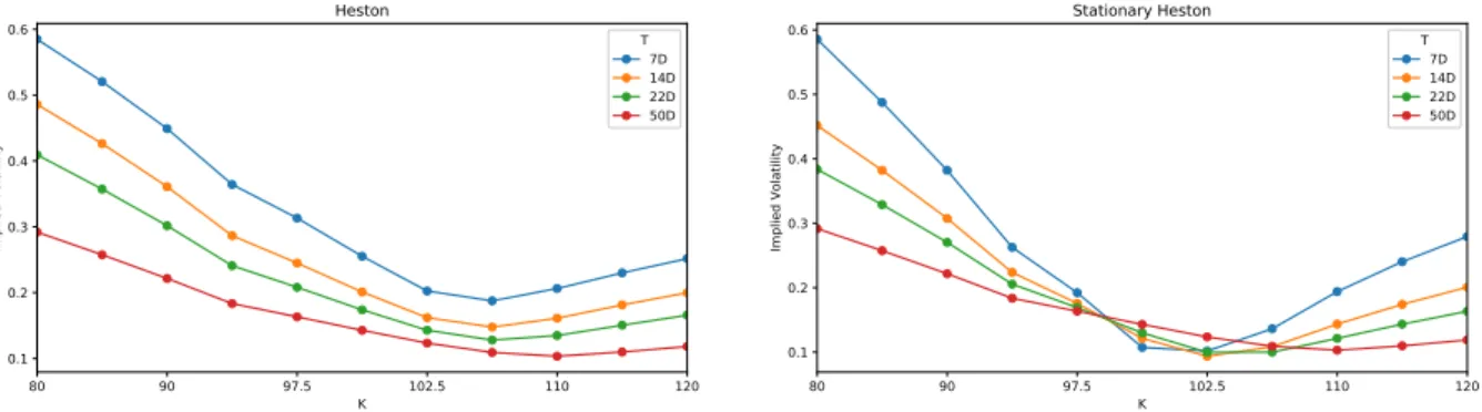
80 90 97.5 102.5 110 120 K 0.1 0.2 0.3 0.4 0.5 0.6 Im pli ed Vo lat ilit y T = 7D T Heston Stationary Heston 80 90 97.5 102.5 110 120 K 0.10 0.15 0.20 0.25 0.30 0.35 0.40 0.45 0.50 Im pli ed Vo lat ilit y T = 14D T Heston Stationary Heston
Figure 3: Implied volatilities for 7 (left) and 14 (right) days expiry options after calibration at 50 days without penalization.
It is clear in Figure 3 that the Standard Heston model fails at producing the desired smile for very small maturities when the Stationary model meets no difficulty to generate it. The next graphics, Figure 4 reproduces the term-structure of the implied volatility in function of T both models.
80 90 97.5 102.5 110 120 K 0.1 0.2 0.3 0.4 0.5 0.6 Im pli ed Vo lat ilit y Heston T 7D 14D 22D 50D 80 90 97.5 102.5 110 120 K 0.1 0.2 0.3 0.4 0.5 0.6 Im pli ed Vo lat ilit y Stationary Heston T 7D 14D 22D 50D
Figure 4: Term-structure of the volatility in function of T and K of both models (left: Standard Heston and right: Stationary Heston) after calibration at 50 days without penalization.
Now, we investigate how these models behave for longer maturities. Do they succeed in preserving the general shape of the market volatility surface or are they only correctly fitting the maturity on which we calibrated them?
Figure 5 represents the relative error between the implied volatility given by the market and the one given by the models calibrated models at 50 days. Clearly, one notices that the Standard Heston model only fits at this expiry. Indeed, when looking at the expiry 22 days or for long-term maturities, the relative error explodes. The term-structure of the implied volatility surface of the market is not preserved when using the Standard Heston model. However, the Stationary Heston model does fit well at both short and long term expiries. The Stationary model produces a steep smile for very short maturities and flattens correctly to the appropriate mean for long expiries.
φ‹ ρ v
0 θ κ ξ
Standard Heston ´0.74 0.152584 0.01487 80.05 5.22
Stationary Heston ´0.75 0.02744 593.46 36.80
Table 1: Parameters obtained for both models after calibration without penalization for options with maturity 50 days (S0 “ 3541, r “ ´0.0032 and q “ 0.00225).
However, looking closely at the parameters obtained after calibration (which are summarized in Table 1), one notices that both sets of calibrated parameters are far from satisfying the Feller condition. And we have to keep in mind that the calibration procedure is performed in order to price path-dependent or American style derivatives using Monte-Carlo simulation or alternative numerical methods, as developed in the next Section. Hence, the Feller condition has to be satisfied, this is the reason why we add a constraint to the minimization problem in order to penalize the sets of parameters not satisfying the condition.
80 85 90 95 97.5 100 102.5 105 110 115 120 22 50 85 113 148 176 267 358 449 631 813 995 1177 1541 1912 2276 2640 3004 3368 T Heston 80 85 90 95 97.5 100 102.5 105 110 115 120 22 50 85 113 148 176 267 358 449 631 813 995 1177 1541 1912 2276 2640 3004 3368 T Stationary Heston 0.06 0.12 0.18 0.24 0.30 0.06 0.12 0.18 0.24 0.30 Figure 5: pK, T q ÝÑ |σivM arketpK,T q´σ M odel iv pφ ‹,K,T q| σM arket iv pK,T q
for both models after calibration at 50 days without penalization. The expiries T are given in days and the strikes K are in percentage of the spot. (left: Standard Heston and right: Stationary Heston).
2.2.2 Optimization with penalization using the Feller condition
The minimization problem becomes
min φPP ÿ K ˆ σM arket iv pK, T q ´ σ M odel iv pφ, K, T q σM arket iv pK, T q ˙2 ` λ maxpξ2´ 2κθ, 0q (2.17)
where λ is the penalization factor to be adjusted during the procedure. The obtained parameters after calibration are summarized in Table 2. The Feller condition is still not fulfilled for both models but it is not far from being satisfied. We choose λ “ 0.01 which seems to be right the compromise in order to avoid underfitting the model because of the constraint.
φ‹ ρ v
0 θ κ ξ
Standard Heston ´0.83 0.0045 0.17023 2.19 1.04
Stationary Heston ´0.99 0.02691 19.28 1.15
Table 2: Parameters obtained for both models after calibration with penalization (λ “ 0.01) for options with maturity 50 days (S0“ 3541, r “ ´0.0032 and q “ 0.00225).
Figure 6 displays the resulting implied volatility curves at 50 days and 22 days for both calibrated models and observed in the market with calibration at 50 days. Adding a penalization term deteriorates the calibration results compared to the non-penalized case (see Figure 2 (right)) but the results are still acceptable.
80 90 97.5 102.5 110 120 K 0.10 0.15 0.20 0.25 0.30 0.35 Im pli ed Vo lat ilit y T = 22D T Market Heston Stationary Heston 80 90 97.5 102.5 110 120 K 0.100 0.125 0.150 0.175 0.200 0.225 0.250 0.275 0.300 Im pli ed Vo lat ilit y T = 50D T Market Heston Stationary Heston
Figure 6: Implied volatilities for 22 (left) and 50 (right) days expiry options after calibration at 50 days with penalization.
Now, again, we extrapolate the implied volatility of both models for very short term maturities in Figure 7. The Stationary Heston model produces the desired smile, however the Standard Heston model fails to produce prices sensibly different than 0 for strikes higher than 105 with this set of parameters, this is why there is no values in implied volatility curves.
80 90 97.5 102.5 110 120 K 0.05 0.10 0.15 0.20 0.25 0.30 0.35 0.40 Im pli ed Vo lat ilit y T = 7D T Heston Stationary Heston 80 90 97.5 102.5 110 120 K 0.05 0.10 0.15 0.20 0.25 0.30 0.35 Im pli ed Vo lat ilit y T = 14D T Heston Stationary Heston
Figure 7: Implied volatilities for 7 (left) and 14 (right) days expiry options after calibration at 50 days with penalization.
Figure 8 represents, as in the non-penalized case, the relative error between the implied volatility given by the market and the one given by the models calibrated models at 50 days using a penalization. The Standard Heston model completely fails to preserve the term-structure while being calibrated at 50 days. In comparison, the Stationary Heston behaves much better and the relative error does not explodes for long-term expiries, meaning that the long run average price variance is well caught.
80 85 90 95 97.5 100 102.5 105 110 115 120 22 50 85 113 148 176 267 358 449 631 813 995 1177 1541 1912 2276 2640 3004 3368 T Heston 80 85 90 95 97.5 100 102.5 105 110 115 120 22 50 85 113 148 176 267 358 449 631 813 995 1177 1541 1912 2276 2640 3004 3368 T Stationary Heston 0.2 0.4 0.6 0.8 1.0 0.2 0.4 0.6 0.8 1.0 Figure 8: pK, T q ÝÑ |σM arketiv pK,T q´σ M odel iv pφ‹,K,T q| σM arket iv pK,T q
for both models after calibration at 50 days with penalization. The expiries T are given in days and the strikes K are in percentage of the spot. (left: Standard Heston and right: Stationary Heston).
3
Toward the pricing of Exotic Options
In this Section, we evaluate first Bermudan options and then Barrier options under the Stationary Heston model. For both products, the pricing rely on a Backward Dynamic Programming Prin-ciple. The numerical solution we propose is based on a two-dimensional product recursive quan-tization scheme. We extend the methodology previously developed by [FSP18, CFG18, CFG17], where they considered an Euler-Maruyama scheme for both components. In this paper, we con-sider a hybrid scheme made up with an Euler-Maruyama scheme for the log-stock price dynamics and a Milstein scheme for the (boosted) volatility process. Finally, we apply the backward algo-rithm that corresponds to the financial product we are dealing with (the Quantized Backward Dynamic Programming Principle for Bermudan Options, see [BP03, BPP05, Pag18] and the algorithm by [Sag10, Pag18] for Barrier Options based on the conditional law of the Brownian motion).
3.1 Discretization scheme of a stochastic volatility model
We first present the time discretization schemes we use for the asset-volatility couple pStpνq, vtνqtPr0,T s.
For the volatility, we choose a Milstein on a boosted version of the process in order to preserve the positivity of the volatility and we select an Euler-Maruyama scheme for the log of the asset.
The boosted volatility. Based on the discussion in Appendix A, we will work with the following boosted volatility process: Yt“ eκtvν
t, t P r0, T s for some κ ą 0, whose diffusion is given
by
dYt“ eκtκθdt ` ξ eκt{2
a
YtdĂWt. (3.1)
The Milstein discretization scheme of Yt is given by
s Ytk`1 “ Mrb,rσ`tk, sYtk, Z 2 k`1 ˘ (3.2)
with tk“ T kn and rb andrσ are given by rbpt, xq “ eκtκθ, r σpt, xq “ ξ?x eκt{2 and rσx1pt, xq “ ξ e κt{2 2?x (3.3) and M rb,rσpt, x, zq defined by M rb,rσpt, x, zq “ x ´ r σpt, xq 2σr1xpt, xq ` h ˆ rbpt, xq ´ prσrσ 1 xqpt, xq 2 ˙ `prσσr 1 xqpt, xqh 2 ˆ z ` ? 1 hrσx1pt, xq ˙2 . (3.4) We made this choice of scheme because, under the Feller condition, the positivity of M
r b,rσ is ensured, since M rb,σrpt, x, zq “ h e κt´κθ ´ξ2 4 ¯ ` hξ 2eκt 4 ˆ z ` 2 ? x ? hξ eκt{2 ˙2 (3.5) and ξ2 ď 2κθ ď 4κθ.
Other schemes could have been used, see [Alf05] for an extensive review of the existing schemes for the discretization of the CIR model, but in our case we needed one allowing us to use the fast recursive quantization, i.e., where we can express explicitly and easily the cumulative distribution function and the first partial moment of the scheme, which is the case of the Milstein scheme (we give more details in SubSection 3.2).
Hence, as our time-discretized scheme is well defined because its positivity is ensured if the Feller condition is satisfied, we can start to think of the time-discretization of our process pStpνqk qkPJ0,nK.
The log-asset. For the asset, the standard approach is to consider the process which is the logarithm of the asset Xt“ logpStq. Applying Itô’s formula, the dynamics of Xt is given by
dXt“ ´ r ´ q ´ vt 2 ¯ dt `?vtdWt. (3.6)
Now, using a standard Euler-Maruyama scheme for the discretization of Xt, we have
# s Xtk`1 “ Eb,σ`tk, sXtk, sYtk, Z 1 k`1 ˘ s Ytk`1 “ Mrb, r σ`tk, sYtk, Z 2 k`1 ˘ (3.7)
where Zk`11 „ N p0, 1q, Zk`12 „ N p0, 1q,CorrpZk`11 , Zk`12 q “ ρ and
Eb,σpt, x, y, zq “ x ` bpt, x, yqh ` σpt, x, yq ? h z (3.8) with bpt, x, yq “ r ´ q ´ e ´κty 2 and σpt, x, yq “ e ´κt{2?y. (3.9)
3.2 Hybrid Product Recursive Quantization
In this part, we describe the methodology used for the construction of the product recursive quantization tree of the couple log asset- boosted volatility in the Heston model.
In Figure 9, as an example, we synthesise the main idea behind the recursive quantization of a diffusion vt which has been time-discretized with F0pt, x, zq. We start at time t0 “ 0 with
a quantizer vp0 taking values in the grid Γt0 “ tv
0
1, . . . , v010u of size 10, where each point is
represented by a black bullet (‚) with probability p0i “Pppv0 “ vi0q is represented by a bar. In
the Stationary Heston model, pv0 is an optimal quantization of the Gamma distribution given
by (1.4) and (1.5). Then, starting from this grid, we simulate the process from time t0 to time
t1 “ 5 days with our chosen time-discretization scheme F0pt, x, zq, yielding rv1 “ F0pt0,pv0, Z1q, where Z1 is a standardized Gaussian random variable. Each trajectory starts from point vi0 with probability p0i. And finally we project the obtained distribution at time t1 onto a grid
Γt1 “ tv
1
1, . . . , v101 u of cardinality 10, represented by black triangles (IJ) such thatpv1is an optimal quantizer of the discretized and simulated process starting from quantizervp0 at time t0“ 0.
Remark 3.1. In practice, for low dimensions, we do not simulate trajectories. We use the information on the law ofvr1 conditionally of starting frompv0. The knowledge of the distribution allows us to use deterministic algorithms during the construction of the optimal quantizer of rv1 that are a lot faster than algorithms based on simulation.
−0.005 0.000 0.005 0.010 0.015 0.020 0.025 t 0.00 0.05 0.10 0.15 0.20 0.25 0.30 vt ̂ v0 ̃ v1= F0(t0, ̂v0, Z1) ̂ v1 v1 i p1 i= ℙ(v1̂= vi1) v0 i p0 i= ℙ(v0̂= v0i)
Figure 9: Example of recursive quantization of the volatility process in the Heston model for one time-step.
In our case, we consider the following stochastic volatility system #
dXt“ bpt, Xt, Ytqdt ` σpt, Xt, YtqdWt
dYt“ rbpt, Ytqdt `rσpt, YtqdĂWt
(3.10)
where Wtand ĂWt are two correlated Brownian motions with correlation ρ P r´1, 1s, b and σ are
defined in (3.9) and rb andrσ are defined in (3.3). Our aim is to build a quantization tree of the couple pXt, Ytq at given dates tk, k “ 0, . . . , n based on a recursive product quantization scheme.
The product recursive quantization of such diffusion system has already been studied by [CFG17] and [RMKP17] in the case case where both processes are discretized using an Euler-Maruyama scheme.
One can notice that building the quantization tree p pYkqkPJ0,nK approximating pYtqtPr0,T s is a
one dimensional problem as the diffusion of Yt is autonomous. Hence, based on our choice of
that was introduced in [PS15] for one dimensional diffusion discretized by an Euler-Maruyama discretization scheme and then extended to higher order schemes, still in one dimension, by [MRKP18]. The minor difference with existing literature is that, in our problem, the initial condition y0 is not deterministic.
Then, using the quantization tree of p pYkqkPJ0,nK we will be able to build the tree p pXkqkPJ0,nK
following ideas developed in [FSP18, RMKP17, CFG18, CFG17]. Indeed, once the quantization tree of the volatility is built, we are in a one-dimensional setting and we are able to use fast deterministic algorithms.
3.2.1 Quantizing the volatility (a one-dimensional case)
Let pYtqtPr0,T s be a stochastic process in R and solution to the stochastic differential equation
dYt“ rbpt, Ytqdt `rσpt, YtqdĂWt (3.11)
where Y0 has the same law than the stationary measure ν: LpY0q “ ν. In order to approximate
our diffusion process, we choose a Milstein scheme for the time discretization, as defined in 3.4 and we build recursively the Markovian quantization tree p pYtkqkPJ0,nKwhere pYtk`1 is the Voronoï
quantization of rYtk`1 defined by r Ytk`1 “ Mrb,rσ`tk, pYtk, Z 2 k`1˘, Ypt k`1 “ ProjΓY N2,k`1 ` r Ytk`1 ˘ (3.12)
and the projection operator ProjΓY
N2,k`1p¨q is defined in (D.2), Γ Y N2,k`1 “ y k`1 1 , . . . , yNk2,k`1 ( is
the grid of the optimal quantizer of rYtk`1 and Z
2
k`1 „ N p0, 1q. In order alleviate the notations,
we will denote rYk and pYk in place of rYtk and pYtk.
The first step consists in building pY0, an optimal quantizer of size N2,0 of Y0. Noticing that
Y0 “ vν0, we use the optimal quantizer we built for the pricing of European options. Then, we
build recursively p pYkqk“1,...,n, where the N2,k-tuple are defined by y1:N2,kk “ `y1k, . . . , yNk2,k ˘
, by solving iteratively the minimization problem defined in the Appendix D in (D.6), with the help of Lloyd’s method I. Replacing X by rYk`1 in (D.6) yields
yk`1j “ E ” r Yk`11Y k`1P Cj ` ΓY N2,k`1 ˘ ı P ´ r Yk`1 P Cj`ΓYN2,k`1 ˘¯ “ E ” M r b,σr `tk, pYk, Zk`12 ˘ 1M r b,σr ` tk, pYk,Zk`12 ˘ P Cj ` ΓY N2,k`1 ˘ ı P ´ M r b,rσ`tk, pYk, Z 2 k`1 ˘ P Cj`ΓYN2,k`1 ˘¯ . (3.13)
Now, preconditioning by pYkin the numerator and the denominator and using pki “P
` p Yk“ yik
˘ ,
we have yjk`1“ E „ E ” M r b,rσ`tk, pYk, Z 2 k`1˘ 1M r b,rσ ` tk, pYk,Zk`12 ˘ P Cj ` ΓY N2,k`1 ˘ | pYk ı E „ P ´ M rb,rσ`tk, pYk, Z 2 k`1 ˘ P Cj`ΓYN2,k`1 ˘ | pYk ¯ “ N2,k ÿ i“1 E ” M r b,rσ`tk, y k i, Zk`12 ˘ 1M r b,rσ ` tk,yki,Zk`12 ˘ P Cj ` ΓY N2,k`1 ˘ ı pki N2,k ÿ i“1 P ´ M r b,rσ`tk, y k i, Zk`12 ˘ P Cj`ΓYN2,k`1 ˘¯ pki “ N2,k ÿ i“1 ´ Kik`yj`1{2k`1 ˘´ Kik`yj´1{2k`1 ˘¯ pki N2,k ÿ i“1 ´ Fik`yj`1{2k`1 ˘´ Fik`yj´1{2k`1 ˘¯ pki (3.14) where Cj`ΓYN2,k`1 ˘
“`yk`1j´1{2, yj`1{2k`1 ‰is defined in (D.1). Fik and Kik are the cumulative distri-bution function and the first partial moment function of Uik „ µki ` κkipZk`11 ` λkiq2 respectively with κkj “ pr σrσ 1 xqptk, yjkqh 2 , λ k j “ 1 ? hrσ 1 xptk, yjkq , and µkj “ yjk´ σptk, y k jq 2rσ 1 xptk, yjkq ` h ˆ rbptk, yjkq ´ prσσr 1 xqptk, yjkq 2 ˙ . (3.15) The functions Fk
i and Kikcan explicitly be determined in terms of the density and the cumulative
distribution function of the normal distribution.
Lemma 3.2. Let U “ µ ` κpZ ` λq2, with µ, κ, λ PR, λ ě 0, κ ą 0 and Z „ N p0, 1q then the cumulative distribution function FX and the first partial moment KU of U are given by
FUpxq “`FZpx`q ´ FZpx´q˘ 1xąµ KUpxq “ ˆ FUpxq`µ ` κpλ 2 ` 1q˘`?κ 2π ´ x´e ´ x2 ` 2 ´x `e ´ x2 ´ 2 ¯˙ 1xąµ (3.16) where x` “ b x´µ κ ´ λ, x´ “ ´ b x´µ
κ ´ λ and FZ is the cumulative distribution function of Z. Finally, we can apply the Lloyd algorithm defined in Appendix D.9 with FX and KX defined by FXpxq “ N2,k ÿ i“1 pki Fikpxq and KXpxq “ N2,k ÿ i“1 pki Kikpxq. (3.17)
In order to be able to build recursively the tree quantization p pYkqk“0,...,n, we need to have
access to the weights pki “P`Ypk “ yik ˘
, which can be themselves computed recursively, as well as the conditional probabilities pkij “P`Ypk`1 “ yjk`1| pYk“ yik
˘ .
Lemma 3.3. The conditional probabilities pkij are given by
And the probabilities pk`1j are given by pk`1j “ N2,k ÿ i“1 pkipkij. (3.19) Proof. The pkij “P`Ypk`1 “ yk`1j | pYk“ yik ˘ “P ´ M rb,rσ`tk, pYk, Z 2 k`1 ˘ P Cj`ΓYN2,k`1 ˘ | pYk“ yki ¯ “P ´ M rb,rσ`tk, y k i, Zk`12 ˘ P Cj`ΓYN2,k`1 ˘¯ “Fik`yk`1j`1{2 ˘ ´ Fik`yj´1{2k`1 ˘ and pk`1j “P`Ypk`1 “ yjk`1 ˘ “ N2,k ÿ i“1 P`Ypk`1 “ yk`1j | pYk“ yik˘ P `pYk “ yki ˘ “ N2,k ÿ i“1 pki pkij.
As an illustration, we display in Figure 10 the rescaled grids obtained after recursive quan-tization of the boosted-volatility, where pvk “ e´κtkYpk and p pYkqk“1,...,n are the quantizers built using the fast recursive quantization approach.
3.2.2 Quantizing the asset (a one-dimensional case again)
Now, using the fact that pYtqt has already been quantized and the Euler-Maruyama scheme of
pXtqt, as defined (3.8), we define the Markov quantized scheme
r Xtk`1 “ Eb,σ`tk, pXtk, pYtk, Z 1 k`1˘, Xpt k`1 “ ProjΓX N1,k`1 ` r Xtk`1 ˘ (3.20)
where the projection operator ProjΓX
N1,k`1p¨q is defined in (D.2), Γ
X
N1,k`1 is the optimal N1,k`1
-quantizer of rXtk`1 and Z
1
k`1 „ N p0, 1q. Again, in order to simplify the notations, rXtk and pXtk are denoted in what follows by rXk and pXk.
Note that we are still in an one-dimensional case, hence we can apply the same methodology as developed in Appendix D and build recursively the quantization`Xpk
˘
Quantizer
vk̂ 0.00 0.05 0.10 0.15 0.20 0.25Time
010 2030 4050 60Pro
ba
bil
ity
p k i 0.00 0.05 0.10 0.15 0.20 0.25 0.30
Figure 10: Rescaled Recursive quantization of the boosted-volatility process with its associated weights from t “ 0 to t “ 60 days with a time step of 5 days with grids of size N “ 10. The recursive quantization methodology is applied to pYk and then we display the rescaled volatility
p
vk“ e´κtkYpk.
where the N1,k-tuple are defined by xk
1:N1,k “`x k 1, . . . , xkN1,k ˘ . Replacing X by rXk in (D.6) yield xk`1j1 “ E ” Eb,σ`tk, pXtk, pYtk, Z 1 k`1˘ 1Eb,σ`tk, pX tk, pYtk,Zk`11 ˘ P Cj1`ΓX N1,k`1 ˘ ı P ´ Eb,σ`tk, pXtk, pYtk, Z 1 k`1 ˘ P Cj1`Γ X N1,k`1 ˘¯ “ N1,k ÿ i1“1 N2,k ÿ i2“1 E ” Eb,σ`tk, xki1, y k i2, Z 1 k`1˘ 1E b,σ ` tk,xki1,yi2k,Z1k`1 ˘ P Cj1 ` ΓX N1,k`1 ˘ ı pkpi 1,i2q N1,k ÿ i1“1 N2,k ÿ i2“1 P ´ Eb,σ`tk, xki1, y k i2, Z 1 k`1 ˘ P Cj1`Γ X N1,k`1 ˘¯ pkpi1,i2q “ N1,k ÿ i1“1 N2,k ÿ i2“1 ´ Kpik1,i2q`xk`1j 1`1{2 ˘ ´ Kpik1,i2q`xk`1j 1´1{2 ˘¯ pkpi1,i2q N1,k ÿ i1“1 N2,k ÿ i2“1 ´ Fpik 1,i2q`x k`1 j1`1{2 ˘ ´ Fpik1,i2q`xk`1j 1´1{2 ˘¯ pkpi 1,i2q (3.21) where pk pi1,i2q “ P ` p Xk “ xki1, pYk “ y k i2 ˘ and Fk pi1,i2q and K k
pi1,i2q are the cumulative distribution function and the first partial moment function of the normal distribution µkpi
1,i2q` Z
1
and they are defined by Fpik 1,i2qpxq “ FZ ˆx ´ µk pi1,i2q σk pi1,i2q ˙ Kpik 1,i2qpxq “ µ k pi1,i2qFZ ˆx ´ µk pi1,i2q σk pi1,i2q ˙ ` σkpi1,i2qKZ ˆx ´ µk pi1,i2q σk pi1,i2q ˙ (3.22) with µkpi 1,i2q“ x k i1 ` bptk, x k i1, y k i2qh and σ k pi1,i2q“ σptk, x k i1, y k i2q ? h (3.23)
and FZ and KZ are the cumulative distribution function and the first partial moment of the standard normal distribution.
Finally, we apply the Lloyd method defined in Appendix (D.9) with FX and KX defined by
FXpxq “ N1,k ÿ i1“1 N2,k ÿ i2“1 pkpi1,i2qFpik1,i2qpxq and KXpxq “ N1,k ÿ i1“1 N2,k ÿ i2“1 pkpi1,i2qKpik1,i2qpxq. (3.24)
The sensitive part concerns the computation of the joint probabilities pk
pi1,i2q. Indeed, they
are needed at each step in order to be able to design recursively the quantization tree.
Lemma 3.4. The joint probabilities pk
pi1,i2q are given by the following forward induction
pk`1pj 1,j2q“ N1,k ÿ i“1 N2,k ÿ j“1 pkpi 1,i2qP ` p Xk`1 “ xk`1j1 , pYk`1 “ y k`1 j2 | pXk“ x k i1, pYk“ y k i2 ˘ (3.25)
where the joint conditional probabilities P`Xpk`1 “ xk`1
j1 , pYk`1 “ y k`1 j2 | pXk “ x k i1, pYk “ y k i2 ˘ are given by the formulas below, depending on the correlation
• if CorrpZ1 k`1, Zk`12 q “ ρ “ 0 P`Xpk`1“ xk`1j 1 , pYk`1“ y k`1 j2 | pXk“ x k i1, pYk“ y k i2 ˘ “ pki2j2 ” N `xk i1,i2,j1,` ˘ ´ N`xki1,i2,j1,´ ˘ı , (3.26) where pki 2j2 is defined in (3.18) and xki1,i2,j1,´ “ xk`1j 1´1{2´ µ k pi1,i2q σk pi1,i2q , xki1,i2,j1,` “ xk`1j 1`1{2´ µ k pi1,i2q σk pi1,i2q , (3.27) with µk pi1,i2q and σ k pi1,i2q defined in (3.23). • if CorrpZ1 k`1, Zk`12 q “ ρ ‰ 0 P`Xpk`1“ xk`1j 1 , pYk`1“ y k`1 j2 | pXk“ x k i1, pYk“ y k i2 ˘ “P ´ Zk`11 P`xki1,i2,j1,´, xki1,i2,j1,`‰, Zk`12 P ´b yk i2,j2,´´ λ k i2, b yk i2,j2,`´ λ k i2 ı¯ `P ´ Zk`11 P`xki1,i2,j1,´, x k i1,i2,j1,`‰, Z 2 k`1 P ” ´ b yk i2,j2,`´ λ k i2, ´ b yk i2,j2,´´ λ k i2 ¯¯ (3.28) where yki2,j2,´ “ 0 _ yjk`1 2´1{2´ µ k i2 κki 2 , yik2,j2,` “ 0 _ yk`1j 2`1{2´ µ k i2 κki 2 , (3.29) with µki 2, κ k i2 and λ k i2 defined in (3.15).
Remark 3.5. The probability in the right hand side of (3.28) can be computed using the cumulative distribution function of a correlated bivariate normal distribution2. Indeed, let
Fρpx1, x2q “PpX1ď x1, X2 ď x2q
the cumulative distribution function of the correlated centered Gaussian vector pX1, X2q with
unit variance and correlation ρ, we have
P`X1P ra, bs, X2P rc, ds ˘ “ Fρpb, dq ´ Fρpb, cq ´ Fρpa, dq ` Fρpa, cq (3.30) with a, c ě ´8 and b, d ď `8. Proof. pk`1pj 1,j2q“P ` p Xk`1 “ xk`1j1 , pYk`1“ y k`1 j2 ˘ “ N1,k ÿ i“1 N2,k ÿ j“1 P`Xpk`1 “ xk`1j 1 , pYk`1 “ y k`1 j2 | pXk“ x k i1, pYk “ y k i2˘ P ` pXk “ x k i1, pYk“ y k i2 ˘ “ N1,k ÿ i“1 N2,k ÿ j“1 pkpi1,i2qP`Xpk`1“ xk`1 j1 , pYk`1 “ y k`1 j2 | pXk“ x k i1, pYk“ y k i2˘. • if CorrpZ1 k`1, Zk`12 q “ ρ “ 0 P`Xpk`1 “ xk`1j 1 , pYk`1 “ y k`1 j2 | pXk“ x k i1, pYk“ y k i2 ˘ “ pki2j2P`Xpk`1 “ xk`1 j1 | pXk“ x k i1, pYk“ y k i2 ˘ “ pki2j2P ´ s Xk`1P`xk`1j1´1{2, xk`1j1`1{2 ‰ | pXk “ xki1, pYk “ y k i2 ¯ “ pki2j2P ´ Eb,σ`tk, xki1, y k i2, Z 1 k`1 ˘ P`xk`1j 1´1{2, x k`1 j1`1{2 ‰¯ “ pki2j2 ” N `xki1,i2,j1,`˘´ N`xki1,i2,j1,´˘ ı , • if CorrpZ1 k`1, Zk`12 q “ ρ ‰ 0 P`Xpk`1 “ xk`1j 1 , pYk`1 “ y k`1 j2 | pXk “ x k i1, pYk “ y k i2 ˘ “P ´ Eb,σ`tk, xki1, y k i2, Z 1 k`1 ˘ P`xk`1j 1´1{2, x k`1 j1`1{2‰, Mrb,rσ`tk, y k i2, Z 2 k`1 ˘ P`yk`1j 2´1{2, y k`1 j2`1{2 ‰¯ “P ´ µkpi 1,i2q` σ k pi1,i2qZ 1 k`1 P`xk`1j1´1{2, x k`1 j1`1{2‰, µ k i2` κ k i2pZ 2 k`1` λki2q 2 P`yjk`1 2´1{2, y k`1 j2`1{2 ‰¯ “P ´ Zk`11 P`xki1,i2,j1,´, x k i1,i2,j1,`‰, pZ 2 k`1` λki2q 2 P`yik2,j2,´, y k i2,j2,` ‰¯ “P ´ Zk`11 P`xki1,i2,j1,´, x k i1,i2,j1,`‰, Z 2 k`1 P ´b yik 2,j2,´´ λ k i2, b yik 2,j2,`´ λ k i2 ı¯ `P ´ Zk`11 P`xki1,i2,j1,´, xki1,i2,j1,`‰, Zk`12 P ” ´ b yik2,j2,`´ λki2, ´ b yki2,j2,´´ λki2 ¯¯ .
2C++ implementation of the upper right tail of a bivariate normal distribution can be found in John Burkardt’s
Remark 3.6. Another possibility for the quantization of the Stationary Heston model could be to use optimal quantizers for the volatility at each date tkin place of using recursive quantization. Indeed, the volatility pvtqt being stationary and the fact that we required the volatility to start
at time 0 from the invariant measure, we could use the grid of the optimal quantizationpv0of size
N of the stationary measure with its associated weights for every dates, hence setting pvk “pv0. We need as well the transitions from time tk to tk`1 defined by
P`pvk`1“ v
k`1
j2 |vpk “ v
k
i2˘. (3.31)
These probabilities can be computed using the conditional law of the CIR process described in [CIJR05, And07], which is a non-central chi-square distribution. Then, we would build the recursive quantizer of the log-asset at date pXk`1 with the standard methodology of recursive
quantization using the already built quantizers of the volatility pvk and the log-asset pXk at time tk, i.e. r Xk`1“ Eb,σ`tk, pXk,pvk, Z 1 k`1 ˘ and Xpk`1 “ ProjΓX N1,k`1 ` r Xk`1 ˘ (3.32)
where, this time, the Euler scheme is not defined in function of the boosted-volatility but directly in function of the volatility and is given by
Eb,σ`t, x, v, z˘ “ x ` h´r ´ q ´ v 2 ¯
`?v?hz. (3.33)
However, the difficulties with this approach come from the computation of the couple tran-sitions P`Xpk`1“ xk`1j 1 ,pvk`1 “ v k`1 j2 | pXk “ x k i1,pvk“ v k i2˘. (3.34)
Indeed, these probability weights would not be as straightforward to compute as the methodology we adopt in this paper, namely using time-discretization schemes for both components. Our approach allows us to express the conditional probability of the couple as the probability that a correlated bi-variate Gaussian vector lies in a rectangle domain and this can be easily be computed numerically.
3.2.3 About the L2-error
In this part, we study the L2-error induced by the product recursive quantization approximation p
Uk “ p pXk, pYkq of sUk“ p sXk, sYkq, the time-discretized processes defined in (3.2) and (3.7) by
s
Uk“ Fk´1p sUk´1, Zkq (3.35)
where Zk“ pZk1, Zk2q is a standardized correlated Gaussian vector and the hybrid discretization scheme Fkpu, Zq is given by
Fkpu, Zq “ ˜Eb,σ`tk, x, y, Zk`11 ˘ M rb,rσ`tk, y, Z 2 k`1 ˘ ¸ . (3.36)
We recall the definition of the product recursive quantizer pUk“ p pXk, pYkq. Its first component
p
Xk is the projection of rXk onto ΓXN1,k and the second component pYk is the projection of rYkonto ΓYN 2,k, i.e., p Xk`1“ ProjΓX N1,k`1 ` r Xk`1 ˘ and Ypk`1 “ ProjΓY N2,k`1 ` r Yk`1 ˘ (3.37)
where rXk and rYk are defined in (3.12) and (3.20), respectively. Moreover, if we consider the
couple rUk“ p rXk, rYkq, using the above notations we have
r
It has been shown in [FSP18, PS18] that if, for all k “ 0, . . . , n ´ 1, the schemes Fkpu, zq are
Lipschitz in u, then there exists constants j “ 1, . . . , n, Cj ă `8 such that
} pUk´ sUk}2 ď k ÿ j“1 Cj`N1,jˆ N2,j ˘´1{2 (3.39)
where pUk and sUk are the processes defined in (3.37) and (3.38). The proof of this result is based
on the extension of Pierce’s lemma to the case of product quantization (see Lemma 2.3 in [PS18]). In our case, the diffusion of the boosted volatility in the CIR model does not have Lipschitz drift and volatility components, hence the above result from [FSP18, PS18] does not apply in our context. Even if we can hope to obtain similar results by applying the same kind of arguments, the results we obtain have to considered carefully. Indeed, when we take the limit in n Ñ `8, the number of time-step, the error upper-bound term goes to infinity. However, in practice, we consider h “ kT {n fixed and then study the behavior of pUk in function of N1,j and N2,j for
j ě k. The proof of the following proposition is given in Appendix C.
Proposition 3.7. Let b, σ, rb and rσ, defined by (3.3) and (3.9), the coefficients of the log-asset and the boosted-volatility of the Heston model. Let, for every k “ 0, . . . , n, pUkthe hybrid recursive
product quantizer at level N1,kˆ N2,k of sUk. Then, for every k “ 0, . . . , n
} pUk´ sUk}2 ď k ÿ j“0 r Aj,k`N1,jˆ N2,j ˘´1{2 ` Bk ? h (3.40) where r Aj,k “ 2 p´2 2p C2 pAj,k ˆ 2pp2´1qjβj p} pU0}p2 ` αp 1 ´ 2pp2´1qjβj p 1 ´ 2p2´1βp ˙1{p (3.41) with Aj,k “ 2 k´j 2 e ? h 2 pk´jq and Bk“ CTphq k´1 ÿ j“0 2k´1´j2 e ? h 2 pk´1´jq (3.42)
where řH“ 0 by convention and CTphq “ Op1q.
3.3 Backward algorithm for Bermudan and Barrier options
Bermudan Options A Bermudan option is a financial derivative product that gives the right to its owner to buy or sell (or to enter to, in the case of a swap) an underlying product with a given payoff ψtp¨, ¨q at predefined exercise dates tt0, ¨ ¨ ¨ , tnu. Its price, at time t0 “ 0, is given by
sup τ Ptt0,¨¨¨ ,tnu E ” e´rτψ τpXτ, Yτq | Ft0 ı
where Xt and Yt are solutions to the system defined in (3.10).
In this part, we follow the numerical solution first introduced by [BPP05, BP03]. They proposed to solve discrete-time optimal stopping problems using a quantization tree of the risk factors Xt and Yt.
Let FX,Y “ pF q0ďkďn the natural filtration of X and Y . Hence, we can define recursively
the sequence of random variable Lp-integrable pVkq0ďkďn
#
Vn“ e´rtnψnpXn, Ynq,
Vk“ max` e´rtkψkpXk, Ykq,ErVk`1 | Fks˘, 0 ď k ď n ´ 1
called Backward Dynamic Programming Principle. Then
V0 “ sup Ere´rτψτpXτ, Yτq | F0s, τ P Θ0,n
(
with Θ0,n the set of all stopping times taking values in tt0, ¨ ¨ ¨ , tnu. The sequence pVkq0ďkďn is
also known as the Snell envelope of the obstacle process ` e´rtkψ
kpXk, Ykq
˘
0ďkďn. In the end,
ErV0s is the quantity we are interested in. Indeed, ErV0s is the price of the Bermudan option
whose payoff is ψk and is exercisable at dates tt1, ¨ ¨ ¨ , tnu.
Following what was defined in (3.43), in order to compute ErV0s, we will need to use the
previously defined quantizer of Xk and Yk: pXk and pYk. Hence, for a given global budget N “
N1,0N2,0` ¨ ¨ ¨ ` N1,nN2,n, the total number of nodes of the tree by the couple p pXk, pYkq0ďkďn, we
can approximate the Backward Dynamic Programming Principle (3.43) by the following sequence involving the couple p pXk, pYkq0ďkďn
# p Vn“ e´rtnψnp pXn, pYnq, p Vk“ max` e´rtkψkp pXk, pYkq,Er pVk`1| p pXk, pYkqs˘, k “ 0, . . . , n ´ 1. (3.44)
Remark 3.8. A direct consequence of choosing recursive Markovian Quantization to spatially discretize the problem is that the sequence p pXk, pYkq0ďkďn is Markovian. Hence p pVkq0ďkďn
de-fined in (3.44) obeying a Backward Dynamic Programming Principle is the Snell envelope of ` e´rtkψ
kp pXk, pYkq
˘
0ďkďn. This is the main difference with the first approach of [BPP05, BP03],
where in there case they only had a pseudo-Snell envelope of` e´rtkψ
kp pXk, pYkq
˘
0ďkďn.
Using the discrete feature of the quantizers, (3.44) can be rewritten
$ ’ ’ ’ ’ ’ & ’ ’ ’ ’ ’ % p vnpxni1, y n i2q “ e ´rtnψ npxni1, y n i2q, i1 “ 1, . . . , N1,n i2 “ 1, . . . , N2,n p vkpxki1, y k i2q “ max ´ e´rtkψ kpxki1, y k i2q, N1,k`1 ÿ j1“1 N2,k`1 ÿ j2“1 πkpi 1,i2q,pj1,j2qvpk`1px k`1 j1 , y k`1 j2 q ¯ , k “ 0, . . . , n ´ 1 i1“ 1, . . . , N1,k i2“ 1, . . . , N2,k (3.45) where πk pi1,i2q,pj1,j2q “ P ` p Xk`1 “ xk`1j1 , pYk`1 “ y k`1 j2 | pXk “ x k i1, pYk “ y k i2 ˘ is the conditional probability weight given in (3.28). Finally, the approximation of the price of the Bermudan option is given by E“pv0px0, pY0q ‰ “ N2,0 ÿ i“1 pipv0px0, y 0 iq (3.46) with pi“P ` p Y0 “ yi0 ˘ given by (2.11).
Barrier Options A Barrier option is a path-dependent financial product whose payoff at maturity date T depends on the value of the process XT at time T and its maximum or minimum over the period r0, T s. More precisely, we are interested by options with the following types of payoff h
h “ f pXTq1tsuptPr0,T sXtPIu or h “ f pXTq1tinftPr0,T sXtPIu (3.47) where I is an unbounded interval ofR, usually of the forme p´8, Ls or rL, `8q (L is the barrier) and f can be any vanilla payoff function (Call, Put, Spread, Butterfly, ...).
In this part, we follow the methodology initiated in [Sag10] in the case of functional quan-tization. This work is based on the Brownian bridge method applied to the Euler-Maruyama
scheme as described e.g. in [Pag18]. We generalize it to stochastic volatility models and product Markovian recursive quantization. Xtbeing discretized by an Euler-Maruyama scheme, yielding
s
Xk with k “ 0, . . . , n, we can determine the law of maxtPr0,T sXst and mintPr0,T sXst given the values sXk “ xk, sYk“ yk, k “ 0, . . . , n L ´ max tPr0,T s s Xt| sXk“ xk, sYk“ yk, k “ 0, . . . , n ¯ “ L ´ max k“0,...,n´1`G k pxk,ykq,xk`1 ˘´1 pUkq ¯ (3.48) and L ´ min tPr0,T s s Xt| sXk“ xk, sYk“ yk, k “ 0, . . . , n ¯ “ L ´ max k“0,...,n´1`F k pxk,ykq,xk`1 ˘´1 pUkq ¯ (3.49)
where pUkqk“0,...,n´1 are i.i.d uniformly distributed random variables over the unit interval and
pGkpx,yq,zq´1 and pFpx,yq,zk q´1 are the inverse of the conditional distribution functions Gk
px,yq,z and Fpx,yq,zk defined by Gkpx,yq,zpuq “ ´ 1 ´ e´2n px´uqpz´uq T σ2ptk,x,yq ¯ 1tuěmaxpx,zqu (3.50) and Fpx,yq,zk puq “ 1 ´ ´ 1 ´ e´2n px´uqpz´uq T σ2ptk,x,yq ¯ 1tuďminpx,zqu. (3.51)
Now, using the resulting representation formula forE f p sXT, maxtPr0,T sXstq (see e.g. [Sag10, Pag18]), we have a new representation formula for the price of up-and-out options sPU O and
down-and-out options sPDO s PU O“ e´rTE“fp sXTq1suptPr0,T sXstďL ‰ “ e´rT E „ f p sXTq n´1 ź k“0 Gk pXk,Ykq, sXk`1pLq (3.52) and s PDO “ e´rT E“fp sXTq1inftPr0,T sXstěL ‰ “ e´rT E „ f p sXTq n´1 ź k“0 ´ 1 ´ Fk p sXk, sYkq, sXk`1pLq ¯ (3.53)
where L is the barrier.
Finally, replace sXk and sYk by pXk and pYk and apply the recursive algorithm in order to
approximate sPU O or sPDO by Er pV0s or equivalentlyErpv0px0, pY0qs
# p Vn“ e´rTf p pXnq, p Vk“E“gkp pXk, pYk, pXk`1q pVk`1 | p pXk, pYkq‰, 0 ď k ď n ´ 1 (3.54)
that can be rewritten $ ’ ’ ’ ’ ’ & ’ ’ ’ ’ ’ % p vnpxni1, y n i2q “ e ´rT f pxn iq, i “ 1, . . . , N1,n j “ 1, . . . , N2,n p vkpxki1, y n i2q “ N1,k`1 ÿ j1“1 N2,k`1 ÿ j2“1 πpik 1,i2q,pj1,j2qpvk`1px k`1 j1 , y k`1 j2 qgkpx k i1, y k i2, x k`1 j1 q, k “ 0, . . . , n ´ 1 i “ 1, . . . , N1,k j “ 1, . . . , N2,k (3.55) with πk pi1,i2q,pj1,j2q “P ` p Xk`1 “ xk`1j1 , pYk`1 “ y k`1 j2 | pXk “ x k i1, pYk “ y k i2 ˘
the conditional proba-bilities given in (3.28) and gkpx, y, zq is either equal to Gkpx,yq,zpLq or 1 ´ Fpx,yq,zk pLq depending on the option type. Finally, the approximation of the price of the barrier option is given by
Er pV0s “E “ p v0px0, pY0q ‰ “ N2,0 ÿ i“1 pipv0px0, y 0 iq (3.56) with pi“P ` p Y0 “ yi0 ˘ given by (2.11).
3.4 Numerical illustrations
In this part, we deal with numerical experiments in the Stationary Heston model. We will apply the methodology based on hybrid product recursive quantization to the pricing of European, Bermudan and Barrier options. For the model parameters, we consider the parameters given in Table 2 obtained after the penalized calibration procedure and instead of considering the market value for S0, we take S0 “ 100 in order to get prices of an order we are used to. For the size of
the quantization grids, we consider grids of constant size for all time-steps: for all k “ 0, . . . , n, we take N1,k “ N1 and N2,k “ N2 where n is the number of time steps. During the numerical
tests, we vary the tuple values pn, N1, N2q.
All the numerical tests have been carried out in C++ on a laptop with a 2,4 GHz 8-Core Intel Core i9 CPU. The computations of the transition probabilities are parallelized on the CPU.
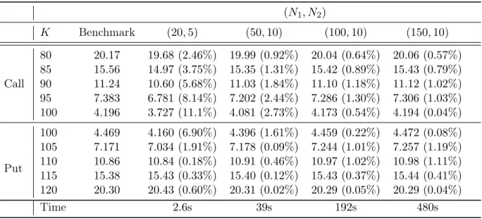
European options First, we compare, in Table 3, the price of European options with maturity tn“ T “ 0.5 (6 months) computed using the quantization tree to the benchmark price computed
using the methodology based on the quadrature formula (the quadrature formula with Laguerre polynomials) explained in Section 2. In place of using the backward algorithm (3.44) (without the function max) for computing the expectation at the expiry date, we use the weights pk
pi1,i2q
defined in (3.25) and built by forward induction, in order to compute
E“ e´rtnψ np pXn, pYnq ‰ “ e´rtn N1,n ÿ i1“1 N2,n ÿ i2“1 ψnpxni1, y n i2q. (3.57)
We give, in parenthesis, the relative error induced by the quantization-based approximation. We compare the behavior of the pricers with different size of grids and numbers of discretization steps. We notice that the main part of the error is explained by the size of the time-step n.
pN1, N2q K Benchmark p20, 5q p50, 10q p100, 10q p150, 10q Call 80 20.17 19.68 p2.46%q 19.99 p0.92%q 20.04 p0.64%q 20.06 p0.57%q 85 15.56 14.97 p3.75%q 15.35 p1.31%q 15.42 p0.89%q 15.43 p0.79%q 90 11.24 10.60 p5.68%q 11.03 p1.84%q 11.10 p1.18%q 11.12 p1.02%q 95 7.383 6.781 p8.14%q 7.202 p2.44%q 7.286 p1.30%q 7.306 p1.03%q 100 4.196 3.727 p11.1%q 4.081 p2.73%q 4.173 p0.54%q 4.194 p0.04%q Put 100 4.469 4.160 p6.90%q 4.396 p1.61%q 4.459 p0.22%q 4.472 p0.08%q 105 7.171 7.034 p1.91%q 7.178 p0.09%q 7.244 p1.01%q 7.257 p1.19%q 110 10.86 10.84 p0.18%q 10.91 p0.46%q 10.97 p1.02%q 10.98 p1.11%q 115 15.38 15.43 p0.33%q 15.40 p0.12%q 15.43 p0.37%q 15.44 p0.41%q 120 20.30 20.43 p0.60%q 20.31 p0.02%q 20.29 p0.05%q 20.29 p0.04%q Time 2.6s 39s 192s 480s
Table 3: Comparison between European options prices, with maturity T “ 0.5 (6 months), given by quantization and the benchmark, in function of the strike K and pN1, N2q where we set
n K Benchmark 30 60 90 180 Call 80 20.17 20.00 p0.83%q 20.03 p0.70%q 20.03 p0.72%q 19.99 p0.92%q 85 15.56 15.33 p1.47%q 15.38 p1.11%q 15.39 p1.07%q 15.35 p1.31%q 90 11.24 10.94 p2.60%q 11.04 p1.78%q 11.05 p1.63%q 11.03 p1.84%q 95 7.383 7.045 p4.57%q 7.170 p2.87%q 7.203 p2.43%q 7.202 p2.44%q 100 4.196 3.879 p7.55%q 4.016 p4.29%q 4.057 p3.31%q 4.081 p2.73%q Put 100 4.469 4.161 p6.89%q 4.306 p3.64%q 4.354 p2.56%q 4.396 p1.61%q 105 7.171 6.972 p2.77%q 7.081 p1.25%q 7.125 p0.64%q 7.178 p0.09%q 110 10.86 10.81 p0.44%q 10.85 p0.05%q 10.87 p0.12%q 10.91 p0.46%q 115 15.38 15.39 p0.06%q 15.38 p0.04%q 15.39 p0.08%q 15.40 p0.12%q 120 20.30 20.29 p0.08%q 20.29 p0.09%q 20.29 p0.06%q 20.31 p0.02%q Time 9s 16s 24s 42s
Table 4: Comparison between European options prices, with maturity T “ 0.5 (6 months), given by quantization and the benchmark, in function of the strike K and of the size n where we set pN1, N2q “ p50, 10q.
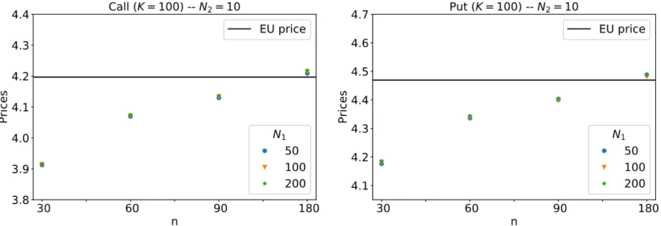
Bermudan options Then, in Figure 11, we display the prices of monthly exercisable Bermu-dan options with maturity T “ 0.5 (6 months) for Call and Put of strikes K “ 100. The prices are computed by quantization and we compare the behavior of the pricer for different choices of time-step n and sizes of the asset grids N1 where we set N2 “ 10. Again, we notice that the choice of n has a high impact on the price given by quantization compared to the choice of the grid size. 30 60 90 180 n 3.8 3.9 4.0 4.1 4.2 4.3 4.4 Pr ic es Call (K = 100) -- N2= 10 EU price N1 50 100 200 30 60 90 180 n 4.1 4.2 4.3 4.4 4.5 4.6 4.7 Pr ic es Put (K = 100) -- N2= 10 EU price N1 50 100 200
Figure 11: Prices of Bermudan options in the stationary Heston model given by product hybrid recursive quantization with fixed value N2“ 10.
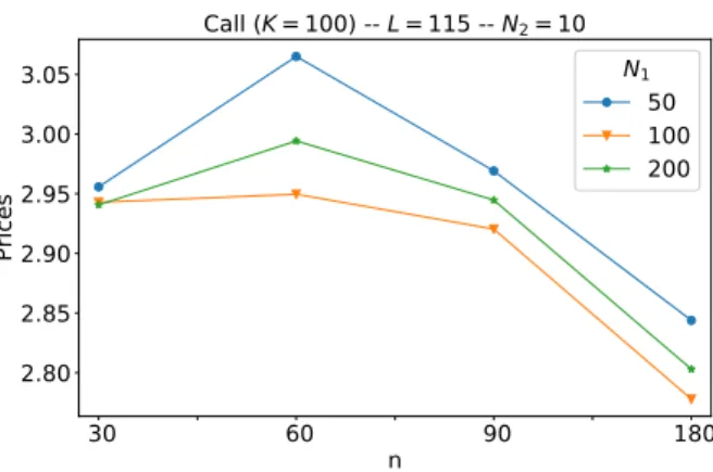
Barrier options Finally, in Figure 12, we display the prices of an up-and-out Barrier option with strike K “ 100, maturity T “ 0.5 (6 months), barrier L “ 115 and N2 “ 10 computed with
30 60 90 180 n 2.80 2.85 2.90 2.95 3.00 3.05 Pr ic es Call (K = 100) -- L = 115 -- N2= 10 N1 50 100 200
Figure 12: Prices of Barrier options with strike K “ 100 in the stationary Heston model given by product hybrid recursive quantization with fixed value N2“ 10.
Acknowledgment
The authors wish to thank Guillaume Aubert for fruitful discussion on the Heston model and Jean-Michel Fayolle for his advice on the calibration of the models. The PhD thesis of Thibaut Montes is funded by a CIFRE grand from The Independent Calculation Agent (The ICA) and French ANRT.
References
[Alf05] Aurélien Alfonsi. On the discretization schemes for the CIR (and bessel squared) processes. Monte Carlo Methods and Applications mcma, 11(4):355–384, 2005.
[AMST07] Hansjörg Albrecher, Philipp Arnold Mayer, Wim Schoutens, and Jurgen Tistaert. The little Heston trap. Wilmott, (1):83–92, 2007.
[And65] Donald G Anderson. Iterative procedures for nonlinear integral equations. Journal of the ACM, 12(4):547–560, 1965.
[And07] Leif BG Andersen. Efficient simulation of the heston stochastic volatility model. SSRN Electronic Journal, 2007.
[BP03] Vlad Bally and Gilles Pagès. A quantization algorithm for solving multidimensional discrete-time optimal stopping problems. Bernoulli, 9(6):1003–1049, 2003.
[BPP05] Vlad Bally, Gilles Pagès, and Jacques Printems. A quantization tree method for pricing and hedging multi-dimensional american options. Mathematical Finance, 15(1):119–168, 2005.
[CFG17] Giorgia Callegaro, Lucio Fiorin, and Martino Grasselli. Pricing via recursive quan-tization in stochastic volatility models. Quantitative Finance, 17(6):855–872, 2017.
[CFG18] Giorgia Callegaro, Lucio Fiorin, and Martino Grasselli. American quantized calibra-tion in stochastic volatility. Risk Magazine, 2018.
[CGP18] Giorgia Callegaro, Martino Grasselli, and Gilles Pagès. Fast hybrid schemes for fractional riccati equations (rough is not so tough). arXiv preprint arXiv:1805.12587, 2018.
[CIJR05] John C Cox, Jonathan E Ingersoll Jr, and Stephen A Ross. A theory of the term structure of interest rates. In Theory of Valuation, pages 129–164. World Scientific, 2005.
[CM99] Peter Carr and Dilip Madan. Option valuation using the fast fourier transform. Journal of computational finance, 2(4):61–73, 1999.
[FSP18] Lucio Fiorin, Abass Sagna, and Gilles Pagès. Product markovian quantization of a diffusion process with applications to finance. Methodology and Computing in Applied Probability, pages 1–32, 2018.
[Gat11] Jim Gatheral. The volatility surface: a practitioner’s guide, volume 357. John Wiley & Sons, 2011.
[GJR18] Jim Gatheral, Thibault Jaisson, and Mathieu Rosenbaum. Volatility is rough. Quan-titative Finance, 18(6):933–949, 2018.
[GJRS18] Hamza Guennoun, Antoine Jacquier, Patrick Roome, and Fangwei Shi. Asymptotic behavior of the fractional heston model. SIAM Journal on Financial Mathematics, 9(3):1017–1045, 2018.
[GL00] Siegfried Graf and Harald Luschgy. Foundations of Quantization for Probability Distributions. Springer-Verlag, Berlin, Heidelberg, 2000.