HAL Id: hal-02968639
https://hal.archives-ouvertes.fr/hal-02968639
Submitted on 16 Oct 2020
HAL is a multi-disciplinary open access
archive for the deposit and dissemination of
sci-entific research documents, whether they are
pub-lished or not. The documents may come from
teaching and research institutions in France or
abroad, or from public or private research centers.
L’archive ouverte pluridisciplinaire HAL, est
destinée au dépôt et à la diffusion de documents
scientifiques de niveau recherche, publiés ou non,
émanant des établissements d’enseignement et de
recherche français ou étrangers, des laboratoires
publics ou privés.
twist to a solar jet from a remote stable flux rope
Reetika Joshi, Brigitte Schmieder, Guillaume Aulanier, Véronique Bommier,
Ramesh Chandra
To cite this version:
Reetika Joshi, Brigitte Schmieder, Guillaume Aulanier, Véronique Bommier, Ramesh Chandra. The
role of small-scale surface motions in the transfer of twist to a solar jet from a remote stable flux
rope. Astronomy and Astrophysics - A&A, EDP Sciences, 2020, 642, pp.A169.
�10.1051/0004-6361/202038562�. �hal-02968639�
https://doi.org/10.1051/0004-6361/202038562 c R. Joshi et al. 2020
Astronomy
&
Astrophysics
The role of small-scale surface motions in the transfer of twist to a
solar jet from a remote stable flux rope
?
Reetika Joshi
1,2, Brigitte Schmieder
1,3,4, Guillaume Aulanier
1, Véronique Bommier
1, and Ramesh Chandra
21 LESIA, Observatoire de Paris, Université PSL, CNRS, Sorbonne Université, Université Paris Diderot, 5 place Jules Janssen, 92190
Meudon, France
e-mail: reetikajoshi.ntl@gmail.com, reetika.joshi@obspm.fr
2 Department of Physics, DSB Campus, Kumaun University, Nainital 263 001, India
3 Centre for mathematical Plasma Astrophysics, Dept. of Mathematics, KU Leuven, 3001 Leuven, Belgium 4 School of Physics and Astronomy, University of Glasgow, Glasgow G12 8QQ, UK
Received 2 June 2020/ Accepted 18 August 2020
ABSTRACT
Context.Jets often have a helical structure containing ejected plasma that is both hot and also cooler and denser than the corona. Various mechanisms have been proposed to explain how jets are triggered, primarily attributed to a magnetic reconnection between the emergence of magnetic flux and environment or that of twisted photospheric motions that bring the system into a state of instability.
Aims.Multi-wavelength observations of a twisted jet observed with the Atmospheric Imaging Assembly (AIA) onboard the Solar Dynamics Observatory and the Interface Region Imaging Spectrograph (IRIS) were used to understand how the twist was injected into the jet, thanks to the IRIS spectrographic slit fortuitously crossing the reconnection site at that time.
Methods.We followed the magnetic history of the active region based on the analysis of the Helioseismic and Magnetic Imager vector magnetic field computed with the UNNOFIT code. The nature and dynamics of the jet reconnection site are characterised by the IRIS spectra.
Results.This region is the result of the collapse of two emerging magnetic fluxes (EMFs) overlaid by arch filament systems that have been well-observed with AIA, IRIS, and the New Vacuum Solar Telescope in Hα. In the magnetic field maps, we found evidence of the pattern of a long sigmoidal flux rope (FR) along the polarity inversion line between the two EMFs, which is the site of the reconnection. Before the jet, an extension of the FR was present and a part of it was detached and formed a small bipole with a bald patch (BP) region, which dynamically became an X-current sheet over the dome of one EMF where the reconnection took place. At the time of the reconnection, the Mg II spectra exhibited a strong extension of the blue wing that is decreasing over a distance of 10 Mm (from −300 km s−1to a few km s−1). This is the signature of the transfer of the twist to the jet.
Conclusions.A comparison with numerical magnetohydrodynamics simulations confirms the existence of the long FR. We conjecture that there is a transfer of twist to the jet during the extension of the FR to the reconnection site without FR eruption. The reconnection would start in the low atmosphere in the BP reconnection region and extend at an X-point along the current sheet formed above.
Key words. Sun: activity – Sun: flares – Sun: magnetic fields
1. Introduction
In the 1990s, jets had already been observed across all tem-perature ranges (104K–107K) in multi-wavelength
observa-tions from Hα with ground-based instruments (Gu et al. 1994; Schmieder et al. 1994, 1995; Canfield et al. 1996) to X-rays with Yohkoh (Shibata et al. 1992). More recently, many jets have been detected in the extreme ultraviolet (EUV) with the Atmospheric Imaging Assembly (AIA, Lemen et al. 2012) onboard the Solar Dynamics Observatory (SDO, Pesnell et al. 2012) and with the Interface Region Imaging Spectrograph (IRIS,De Pontieu et al. 2014). Their characteristics vary in wide parameter ranges, such as velocity (100–400 km s−1),
exten-sion (104–106km), and width (104–105km) (Nisticò et al. 2009;
Schmieder et al. 2013;Joshi et al. 2017).
Exhibiting a twist or rotation is a common property for jets overall (Raouafi et al. 2016). The twist of the jet may be due
? Movies attached to Figs. 1, 3, 4, and 7 are available at
https://www.aanda.org
to helical motions (Nisticò et al. 2009;Patsourakos et al. 2008). Twisting motions have been found in a large velocity range of jets or surges (Chen et al. 2012; Hong et al. 2013; Zhang & Ji 2014). In the study done bySchmieder et al.(2013), a jet analy-sis revealed a striped pattern of dark and bright strands propagat-ing along the jet, as well as apparent damped oscillations across the jet. They concluded that this is suggestive of a (un)twisting motion in the jet, possibly an Alfvén wave. Spectroscopic data also provide signatures for detecting the twist in jets. For exam-ple, blue and red shifts observed along the axis of a jet in Hα as well as in Mg II lines were interpreted as confirmation of the existence of twist along the jet (Ruan et al. 2019).
The concept behind the existence of coronal jets is based on magnetic reconnection. This was first proposed by Heyvaerts et al. (1977) and simulated by Shibata et al. (1982, 1992) andYokoyama & Shibata(1996). Magnetic reconnection has explained the X-ray jets observed by Yohkoh (Shimojo et al. 1996; Shimojo & Shibata 2000; Asai et al. 2001). It also sup-ports the interpretation of jets observed in multi-wavelengths from X-ray (Shimojo et al. 1996; Shimojo & Shibata 2000;
Open Access article,published by EDP Sciences, under the terms of the Creative Commons Attribution License (https://creativecommons.org/licenses/by/4.0),
Asai et al. 2001) to EUV (Schmieder et al. 1983, 1988, 1994; Chae et al. 1999;Nisticò et al. 2009;Chandra et al. 2017). Spec-troscopic and imaging observations of small-scale events reveal bidirectional flows in transition region lines at the jet base which could correspond to an explosive reconnection (Li et al. 2018; Ruan et al. 2019). There are different conditions for the magnetic configuration of an active region (AR) to trigger magnetic recon-nection. We may quote three types of conditions: magnetic flux emergence (Archontis et al. 2004, 2005; Moreno-Insertis et al. 2008; Török et al. 2009; Moreno-Insertis & Galsgaard 2013), magnetic flux cancellation (Priest et al. 2018; Syntelis et al. 2019), and magnetic instability (Pariat et al. 2010,2015,2016). The first two mechanisms predict hot and cool jets simulta-neously. However, the presence of surges and jets is not fre-quently reported. Some papers report on the X-ray jets observed by Yohkoh and associated with a surge (Schmieder et al. 1995; Canfield et al. 1996; Ruan et al. 2019). Radiative magnetohy-drodynamics (MHD) simulations based on flux emergence (Nóbrega-Siverio et al. 2016,2017) as well as the flux cancel-lation model (Syntelis et al. 2019) show that surges can exist at the same time with hot jets. The cool plasma is advected over the emergence domain without passing near the reconnection site and then flows along the reconnected magnetic field lines. These models fit with the observations of X-ray jets observed with Hinode and with Hα jets from the Swedish 1-m Solar Tele-scope (SST) (Nóbrega-Siverio et al. 2017). Recently,Joshi et al. (2020) presented a case-study of collimated hot jets and asso-ciated cool surges which fit in perfectly with the simulation of jets formed by flux emergence. The double-chambered struc-ture found in the observations corresponds to the cool and hot loop regions found under the reconnection site in the models of Moreno-Insertis et al.(2008). Jets can also be the consequence of magnetic instability. Firstly, we see there is the storage of energy by twisted field lines or shearing of polarities. Suddenly, the system becomes unstable with a disruption of the field lines via reconnection occurs and material expelled along the open magnetic field lines. This mechanism is based on a twisted flux rope (FR) formation during the shear in the jet region (Yeates & Hornig 2011; Pariat et al. 2015, 2016; Raouafi et al. 2016). The slow reconnection is driven by the response of the system to continual stressing of the closed field injecting mag-netic helicity. When the kink instability encompasses the entirety of the closed field region, it leads to a large jet eruption. In the model ofWyper et al.(2019), the overlying magnetic field is, in fact, expelled by a gentle reconnection above the closed AR via a breakout mechanism before the instability occurs.Pariat et al. (2015), andWyper et al.(2019) show the importance of the incli-nation of jets favouring the jet onset for θ= 0–20 degrees. These models are based on the instability of the system; a FR formed by shear under the reconnection point is the trigger of the heli-cal jet. However, based on several observations, it becomes clear that the twist is not present before the reconnection but the twist of the jet is transferred during the reconnection. For example, in Ruan et al.(2019), the twist was transferred from twisted overly-ing magnetic field lines remnant of the eruption of a filament two hours before the onset of the jet. The null-point is the favourable location for the occurrence of magnetic reconnection.
Wyper et al. (2019) recently showed that reconnection can be in a region where the magnetic field lines are tangent to the photosphere. This kind of region is called bald patch (BP) region. It favours reconnection as a mechanism for ini-tiating jets and surges (Mandrini et al. 2002; Chandra et al. 2017; Zhao et al. 2017). In these studies, the magnetic topol-ogy was derived by linear force free field (LFFF) or non
linear force free field (NLFFF) magnetic field extrapolations in the corona (Mandrini et al. 2002; Chandra et al. 2017) or by directly analysing the observed magnetic field vector maps (Bernasconi et al. 2002;Zhao et al. 2017). The occurrence of the reconnection was clearly taking place in the BP regions. It was also recently proposed that the trigger of jets can be due to the eruption of mini-filament at the jet base (Sterling et al. 2016). That model fits well with the blowout jets where the entire region below the dome of reconnection is expelled during the eruption (Moore et al. 2010).
In this paper, we present observations of a twisted jet, a surge, and a mini-flare which occurred on 22 March 2019 at 02:05 UT observed in multi-wavelengths with AIA, IRIS instru-ments, and with the New Vacuum Solar Telescope (NVST, Liu et al. 2014) in Fuxian Solar Observatory of Yunnan Astro-nomical Observatory, China1(Sects.2.1and2.4). The IRIS spec-tra at the reconnection site display a tilt and gradient in the spectra along the jet base indicating the formation of a rotat-ing structure durrotat-ing the reconnection (Sect.3.3). In Sect.4, we analyse the magnetic topology of the AR. This region with the mini-flare was recently studied by an other group (Yang et al. 2020) and independently of our study. They performed a NLFFF extrapolation to show that the region has a fan-spine magnetic topology with two FRs. They proposed a break-out model which might remove the overlaying arcades, leaving a small FR to erupt and turn into a blowout jet – as in the scenario ofSterling et al. (2016) and in the model ofWyper et al.(2017).
In Sect. 4.1, our detailed consideration of the EUV data based on the analysis of the photospheric vector magnetic field obtained with the 12 min cadence Helioseismic and Magnetic Imager (HMI,Schou et al. 2012) leads us to a different interpre-tation for the event. The clues that support our interpreinterpre-tation are the identification of a non-eruptive FR, from which some twist is carried away, eventually reconnecting into the jet at the “X” point of the current sheet that is dynamically formed from a BP current sheet underneath. The presence of the FR is supported by a relatively good accordance that can be seen for the patterns of transverse fields and vertical current densities, as observed by HMI, and appearing without being constrained a priori in an MHD simulation of non-eruptive FR formation with flux-cancellation of sheared loops (Zuccarello et al. 2015), carried out with the Observationally driven High-order scheme Mag-netohydrodynamic (OHM) code (Aulanier et al. 2005, 2010) (Sect.4.2). The transport of twist away from the FR towards the “X” point is supported by HMI observations of a moving neg-ative flux-concentration whose transverse fields point towards a positive one. In Sect.5, we discuss the two interpretations and conclude our scenario based on HMI and IRIS observations.
2. Instruments
2.1. AIA
In the active region (AR) NOAA 12736, a jet as well as a surge is well-observed in the multi-wavelength filters of AIA aboard SDO. The AIA data consists of a sample of filters with passbands centered at different lines emitting at different temperatures from 304 Å(He II, T ∼ 0.05 MK), 171 Å(Fe IX, T ∼ 0.6 MK), and 193 Å(Fe XII, T ∼ 0.6 MK) to hotter temperatures of 94 Å (Fe XVIII, T ∼ 6.3 MK), 131 Å(T1 = 10 MK and T2 = 0.64 MK),
and 211 Å(T1∼ 20 MK and T2∼ 1.6 MK). The AIA data cadence
in these channels is 12 s and the pixel size is 0.600.
2.2. HMI
The longitudinal magnetic field is provided by the HMI team with a cadence of 45 s and a pixel size of 0.500. To obtain
the magnetic field vectors in full, we inverted the HMI level-1p IQUV data, averaged on a 12 min cadence, by applying the Milne-Eddington inversion code UNNOFIT (Bommier et al. 2007). We selected a large area covering the AR 12736 and applied a solar rotation compensation to select the same region over more than six hours of observation. We thus treated 22 maps from 21 March 2019 at 23:00 UT to 22 March 2019 at 03:12 UT and three later maps of the same region from 05:00 UT to 05:24 UT. The specificity of UNNOFIT is that a magnetic fill-ing factor is introduced to take into account the unresolved mag-netic structures as a free parameter of the Levenberg-Marquardt algorithm that fits the observed set of profiles with a theoretical one. However, for further application, we used only the averaged field, that is, the product of the field with the magnetic filling factor, as recommended byBommier et al.(2007). The interest of the method lies in a better determination of the field inclina-tion. After the inversion, the 180◦remaining azimuth ambiguity was resolved by applying the ME0 code developed by Metcalf, Leka, Barnes, and Crouch (Leka et al. 2009)2. After resolving the ambiguity, the magnetic field vectors were rotated into the local reference frame, where the local vertical axis is the ozaxis.
2.3. NVST
The Hα observations were taken with the NVST telescope, pointed at the AR 12736 at N09 W60 on 22 March 2019 from 00:57:00 UT to 04:37:00 UT. We used the line–center Hα obser-vations at 6562.8 Å that were obtained in a field of view (FOV) of 12600× 12600with a cadence of 29 s. The Hα movie for these
observations is available online3. It displays the Hα fine struc-tures and shows their evolution very well. For the current anal-ysis, we used the level 1+ data provided by the NVST team. To focus on the jet region, we cut the data cube after rotating it with north upwards, as in the space data (AIA and HMI observations) and used the data of FOV of 6500× 6500.
2.4. IRIS
The IRIS FOV was focused on AR NOAA 12736 and the point-ing of the telescope was at 70900, 22800with a FOV of 6000× 6800
for the slit-jaw images (SJIs). The observational characteristics are presented in Table1. We used the 1330 Å and 2796 Å SJIs for this study. There was no data for the IRIS SJI Si IV 1400 filter. The SJI 1330 Å includes the CIIline formed at T = 30 000 K, and the SJI 2796 Å emission mainly comes from the MgIIk line. The MgIIh and k lines are formed at chromospheric tempera-tures, that is, between 8000 K and 15 000 K (De Pontieu et al. 2014;Alissandrakis et al. 2018). The co-alignment between the different optical channels of IRIS was achieved by using the drot_map in solar software to correct the differential rotation. The SJIs in the broadband filters (1330 Å, and 2796 Å) were taken at a cadence of 14 s.
With IRIS, medium coarse rasters of four steps were per-formed from 01:43:27 UT to 02:42:30 UT on 22 March 2019. The raster step size is 200 so that each spectral raster spans a field of view (FOV) of 600× 6200. The nominal spatial
resolu-tion is 0.0033. IRIS provides line profiles in Mg II k 2796.4 Å
2 Available athttp://www.cora.nwra.com/AMBIG/ 3 http://fso.ynao.ac.cn/datashow.aspx?id=2296
Table 1. IRIS observation of AR NOAA 12736 on 22 March 2019.
Location Time Raster SJI
(UT) x= 70900 01:43 to FOV: 600× 6200 FOV: 6000× 6800 y= 22800 02:42 Steps: 4 × 200 C II 1330 Å Spatial Mg II 2796 Å Resolution: 0.0033 Time Cadence: 3.6 s Resolution: 14 s and Mg II h 2803.5 Å, Si IV (1393.76 Å, 1402.77 Å) and C II (1334.54 Å, 1335.72 Å) lines along four slit positions (200 pix-els) and repeated 250 times. Calibrated level 2 data were used in this study. Dark current subtraction, flat field correction, and geometrical correction have been taken into account in the level 2 data (De Pontieu et al. 2014).
3. Observations
3.1. Birth of the active region
A mflare (B6.7 X-ray class) and its associated jet was ini-tiated in AR NOAA 12736 located at N09 W60 on 22 March 2019 around 02:02 UT. The magnetic field evolution and AIA observations of the AR are presented in Sects.3.1.1and3.1.2 respectively.
3.1.1. Magnetic field
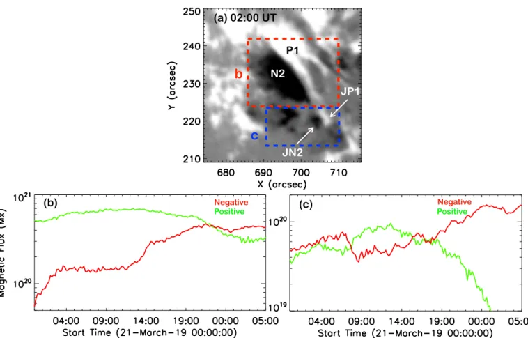
The AR 12736 was emerging progressively since 19 March 2019. On 21 March, we note two emerging flux regions (EMFs) elongated along the north-east to south-west direction (see the ovals in Figs.1b and d). The first emerging flux region (EMF1) is the main component of the AR, with negative leading polar-ity and positive following polarpolar-ity. The second emerging flux region (EMF2) consists of many fragmented negative polarities which are travelling very fast as the emerging flux is expand-ing towards south and squeeze the positive polarity of EMF1. Consequently, a very high magnetic field gradient is observed perpendicularly to the polarity inversion line (PIL) between the squeezed polarities: “P1” positive polarity belonging to EMF1 and “N2” negative polarity belonging to EMF2 (see the red box in Fig.1e). The negative polarity N2 is surrounded by positive polarities P1 on the right side and P2 on the left side and top. This topology is classical with the aim of getting a null point, as we see discuss further on in this paper. In the HMI movie (ani-mation is attached as MOV1), we note the fast sliding motion of negative polarity N2 towards the south and the motion of positive polarity P1 in the opposite direction, which creates a strong shear between them. Along this PIL, we distinguish that at the time of the flare observations, we principally observe two bipoles ema-nating from the two EMFs in the diagonal of the box (NE-SW): a large north bipole (P1, N2) and a very tiny bipole (JP1, JN2) in the south, which was detached progressively from the north-ern N2 polarity a few hours before (the animation is attached as MOV1 and explained in Sect.4). We computed the flux budget for these two bipoles and we found a significant decrease of the positive flux in the two boxes, each of them including a bipole (Fig. 2). We interpret these decreases by magnetic cancelling flux. The tiny bipole is labeled with “J” like “jet” because this is the location where the jet took place.
N1
P1
N2
P2
P1
N2
P2
N1
Fig. 1.Panels a–e: HMI longitudinal magnetograms of AR NOAA 12736 showing the evolution of the magnetic polarities. The jet reconnection is occurring between the two large emerging flux areas EMF1 (P1, N1) and EMF2 (P2, N2) encompassed in the two ovals drawn in panels b and d. The emergence of the EMFs is shown by the extension of the two ovals between these two times. Panel f: HMI continuum image showing the sunspots and pores of the AR. The blue and green contours are for negative, and positive magnetic field polarities with label ±300 Gauss. The red rectangular box in panel e shows the FOV of Figs.2a and11a and b.
3.1.2. Arch filament systems (AFS)
The AIA observations cover the AR and the full development of the jet in multi-temperatures provided by all the sample of AIA filters from 304 Å to 94 Å, all along the range of tempera-tures from 105K to 107K (Figs.3and4 along with the related
movies (animations are attached as MOV2a-d in AIA 131 Å, 171 Å, 211 Å, and 304 Å). Contours of longitudinal magnetic fields (±300 Gauss) are overlaid on the AIA images to specify the location of the small bipole JP1-JN2 at the jet base. AFS are well visible over the two emerging flux EMF1 and EMF2 with cool and hot low lying loops joining the positive and negative polarities for each of them, P1 and N1 on the west side and P2 and N2 on the east side. Filaments belonging to these AFS are particularly visible as dark structures due to absorption mecha-nism in 171 Å, 131 Å, and 193 Å at 02:06 UT (Fig.3panel e and Fig.4 panels b, e). These filaments are parallel to each other, oriented more or less NE to SW from P1 to N1 and from P2 to N2 in the direction of the extension of each EMF. They do not lie along any PIL and, therefore, they do not correspond to the usual definition of filaments; rather, they are more or less perpendic-ular to the PIL in each EMF. Filters AIA 171 Å and 193 Å are good proxies for detecting cool structures visible in Hα. At these wavelengths, the EUV emission is absorbed by the hydrogen and helium continua (Anzer & Heinzel 2005). The opacity of the hydrogen and helium resonance continua at 171 Å is almost two orders of magnitude lower than the Lyman continuum opacity at 912 Å and thus similar to the Hα line opacity (Schmieder et al. 2004). We confirm the presence of Hα filaments/AFS by look-ing at the Hα images (Fig.5). The two AFS over the two EMFs are well identified. On the west side the AFS are dense and long,
with some narrow arch filaments overlying the bright corridor of the PIL (N2-P1) and the dome of EMF2 before the burst (panel b). The AFS over EMF2 on the east side have a fan structure with an anchorage all around the negative polarities N2 and the other in the positive polarities P1 and P2. It gives the impression of an “anemone” structure which is frequently observed for jets triggered by emerging flux (Shibata et al. 1982;Schmieder et al. 2013;Joshi et al. 2020). In order to follow the jet development with AIA, we focus on the FOV covering the two bipoles identi-fied in the previous section. For more details, see the white box in Fig.3a.
3.2. Observations of the jet 3.2.1. Jets in AIA images
It is interesting to see that activity had started before the onset of the jet, with very bright north-south tiny threads observed above the PIL between the two EMFs and, more precisely, between the part of the PIL in the northern bipole (P1-N2) and continu-ing into the south tiny bipole (JP1-JN2) around 02:01 UT until 02:04 UT. See the inserted zoom image in Fig.4g.
The bright signature around a dome structure overlying the EMF2 at the jet base is highlighted by a white dashed con-tour around it, as seen in Fig. 4e. This dome is highlighted by the small fibrils with an asymmetrical anemone shape visi-ble in the NVST images (Fig. 5b). Along the west side of the dome, the brightening with an north-south arch-shape is visi-ble in all AIA channels before the burst indicates already the presence of hot plasma (T between 104–106K). This region
between the two EMFs corresponds to quasi-separatrix lay-ers (QSLs;Démoulin et al. 1996), where a strong high electric
JN2 N2 Positive Negative Positive Negative (b) (c) N2 JP1 JN2
c
N2 P1b
(a) 02:00 UT JN2 JP1 N2Fig. 2.Magnetic flux cancellation in two areas including the major bipole (P1, N2) (red box (b)) and the small jet bipole (JP1, JP2) (blue box (c)), respectively. Panel a: a zoom of the longitudinal magnetic map including the two bipoles (FOV is the red box in Fig.1e). Panels b, c: variation of the magnetic flux in the red and blue boxes.
current develops and heats the plasma, as shown here by the arch-shape brightening. This is subsequently confirmed with the analysis of the photospheric vector magnetic field maps in Sect.4. These QSLs have been calculated inYang et al.(2020) and are well-identified in this region. QSLs are robust structures but their localisation is not commonly defined with any sub-stantial accuracy (Dalmasse et al. 2015;Joshi et al. 2019). In our case, the moving polarities is a problem for the exact localisation of QSLs.
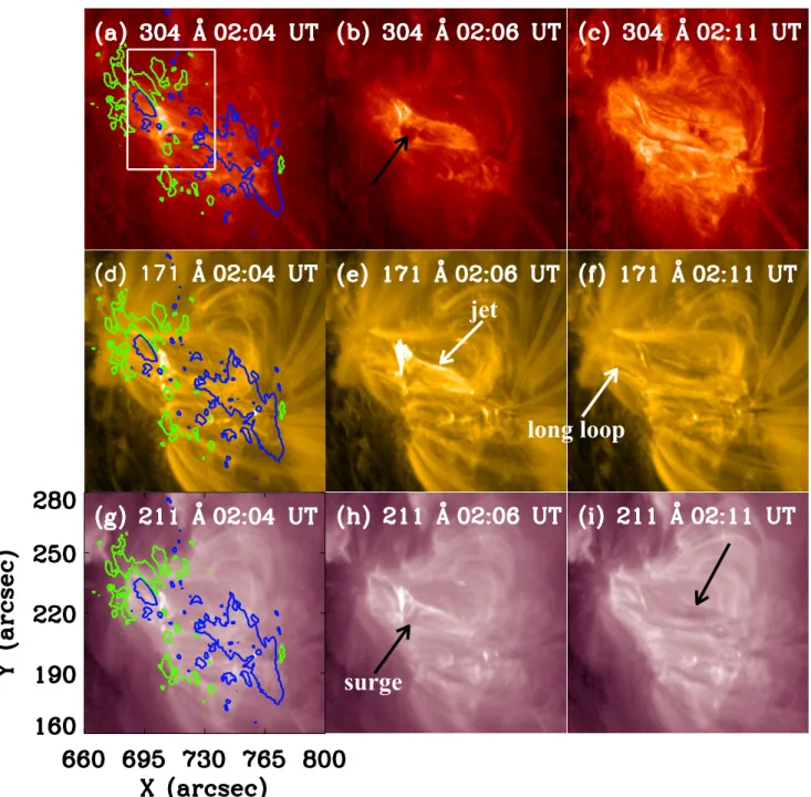
At the same time (02:04 UT), a jet with two branches insert-ing a surge is also observed. Dark absorbinsert-ing material is visible at ≈02:02 UT, resembling a blob with no really defined shape in the southern part of the arch-shaped brightening (see Fig.5panel c). It then extends to the north and, finally, goes along the jet direc-tion. The surge appears as a dark area in the images because of the absorption of the UV emission. Therefore, the dark part observed in 171 Å and in the other AIA filters, that is, (211, 193, 94 Å) should correspond to cool plasma as seen in Hα as we mentioned in the previous section (Schmieder et al. 2004). It is why we call it a “surge” (Figs.3 and4). The surge appears as a bright structure in the NVST images (Fig.5e). However, the surge consists of cool plasma because Hα formation temperature is lower than 1.5 × 10⁴K.
The jet base on the east side of the EMF1 is extended along a more or less north-south direction, along the PIL between EMF1 and EMF2 (P1 and N2; see Fig. 4g) and the jet top on the west side of the EMF1 is limited at the location of N1. At 02:11 UT and over a few minutes up until 02:18 UT, we can observe long bright and dark AFS striding over the two EMFs
(see right columns of Figs.3and4). The characteristics of the jet are the following: length around 50 Mm, the base width between 15–20 Mm. The jet lifetime is between 02:02 UT to 02:11 UT.
In AIA, a 304 Å movie starting at 20:00 UT on 21 March 2019 and running until 22 March 2019 at 05:00 UT, we made several observations of a mini-flare, approximately at the same location, nearly one every hour and generally not accompanied by such a wide jet. The detail of the recurrent mini-flares is as follows: at the beginning of the movie, a mini-flare is visible at 20:00 UT, then at 20:27 UT, 21:28 UT, 22:51 on 21 March and at 00:39 UT, 01:25 UT, 01:39 UT, 02:03 UT on 22 March. Regularly, before each burst, we can clearly see two AFSs: one over EMF1 in the west and one over EMF2 in the east. After the burst, long-arch filaments connect the extreme eastern polarity P2 to the extreme western polarity N1. Prior to our mini-flare and jet (around 01:59 UT), the two AFSs were separated by an area with mixed bright and dark patches. Then at 02:09 UT, there is a long system of arch filaments. At 02:28 UT, when the phase of the activity is over, the initial configuration with the two dis-tinguished AFSs, just as before the jet, is restored. This chain of mini-flare and ejection is recurrent.
3.2.2. Transverse projected velocity
To analyse the kinematics of the observed jet, we created the projected height-time profiles of the jet in different AIA wave-bands (171 Å, 211 Å, and 304 Å), which is presented in Fig.6. To obtain this height-time plot, we chose a broad slit (width= 8 pixels) to cover the plasma outflow. The average jet speed along
jet
long loop
surge
Fig. 3.Solar jet and surge observed in different AIA/EUV channels (304 Å, 171 Å, and 211 Å) on March 22 2019 between 02:04 UT and 02:11 UT
in NOAA AR 12736. The black arrows in (b) and (h) indicate a dark area corresponding to a surge, the white arrow points the jet in (e) and a long loop created after the reconnection in (f ), the black arrow in (i) an AFS. In the first column the images are overlaid with HMI longitudinal magnetic field contours (±300 Gauss) for positive and negative magnetic polarities with green and blue colours, respectively. The white box in panel aindicates the FOV of Fig.7. The small bipole center is at 71000
, 22000
, and the major bipole center is at 69500
, 23000
.
the slit direction shows two different slopes: a steep slope in the starting phase (till 02:0 UT) of the jet eruption with an average speed of 350 km s−1 and a slow phase of 80 km s−1 in the later stage from 02:05 UT to 02:08 UT. The slow phase may be due to the presence of loop system in the path of the jet. It seems that when the jet material is passed through this loop system, it decelerated and, finally, it stopped.
The cool material visible as an absorbing feature in AIA channels is detected about one minute after the hot jet with no well defined speed. The cool material appears to be present along the line of sight in small patches but it is not moving towards the west as the jet is doing. Later, the cool material (or surge)
is escaping in slightly different directions than the jet. Among it, we could identify some blobs with different projected speeds (≈100 and 30 km s−1). Then the cool material came back at a speed of ≈ −40 km s−1 (Fig 6d). According to the location of
the AR (W60), these velocities are underestimated by a factor of cos(60). The positive velocities correspond to the material that is heading away from the observer’s view.
3.3. Corresponding structures in IRIS SJIs and AIA 304 Å The analysis of IRIS data, all along the evolution of the jet, shows a good correspondence between the structures visible in
Fig. 4.Solar jet and surge observed in the other AIA/EUV channels (131 Å, 193 Åand 94 Å). The first column shows the images overlaid with HMI
longitudinal magnetic field contours (±300 Gauss) for positive and negative magnetic polarities with green and blue colours, respectively. Panel e shows a dome structure at the jet base highlighted by a white dashed contour. In panel g, the red box shows the field of view of the brightening at the jet base overlaid by the contours of the small bipole (71000
, 22000
) and the large bipole (69500
, 23000
).
AIA 304 Å and in IRIS CII SJIs (animations are attached as MOV2d (AIA 304 Å), and MOV3 (IRIS 1330 Å)). This corre-spondence is summarised in Fig. 7. We note that the nominal coordinates of IRIS in the file headers do not correspond to the nominal coordinates of AIA. Therefore, we had to shift the FOV of AIA by 4 arcsec in x-axis and 3 arcsec in y-axis to obtain a good co-alignment. The IRIS slit, with its four positions, crosses the bright zone corresponding to the jet base, namely, the dome top, which is supposed to be the reconnection site along a few pixels between around pixels 60 to 120 in the left slit position (Fig.7e).
Around 02:00 UT, in the 304 Å image as well as in CIIand MgII IRIS SJIs, small bright threads along two vertical paths that are mixed with tiny round-shape darker areas are visible in the middle of the FOV where the reconnection occurred (Fig.7a, d, and g). It is clear that in this small zone, there is no
north-south filament along the PIL (N2-P1) which would be visible by absorption in AIA 193 Å. The very light-dark filament-type structure with a vague sigmoidal shape in the NVST images that is localised at this place is, in fact, part of the AFS (see Fig.5b) because there is no sigmoid visible in the hot channels of AIA, where plasma should be heated due to high electric cur-rents along a sigmoid (Barczynski et al. 2020). In the north of this zone, long-lying, more or less east-west AFS, as well as, on both sides of the zone (pixels 60–120), the short AFS-overlying EMF1 and EMF2 are visible. The short AFS-overlying EMF2 have a dome shape like the asymmetrical anemone formed by the fibrils visible in the NVST images (Fig.5).
The location of the onset of the mini-flare is indicated by the point “X” at the crossing location between the arch-shape QSL and an east-west bright line in Fig.7d). The location of the “X” point in IRIS observation is at 70900, 21800 and in AIA
JP1
JN2
N1
P1
P2
(a) 02:00 UT
(b) 02:01 UT
(c) 02:03 UT
AFS2
FilamentArchAFS1
blob
X
surge
long AFS
(d) 02:04 UT
(e) 02:05 UT
(f) 02:15 UT
Fig. 5.Hα line center observations of the AR NOAA 12736 with the NVST telescope for four times before (a-d) and one after (f ) the surge extension. In panel a, the cyan oval encircles the emerging flux EMF2 like in Fig.1which corresponds to a dome (see Sect.3.2.1), the green circle indicates the bipole P1-N2, the black circle the bipole JP1-JN2. In panel b, we highlight the two systems of AFS (AFS1 and AFS2), with the white arrows indicating long AFS overlying both AFS1 and AFS2 structures. In panel c, we see a dark blob in the middle of the brightening. In panel dthe “X” point is indicated where the reconnection occurs. In panel e, the white, more or less horizontal material represents the beginning of the surge ejection with some knots. In panel f, we again see the long AFS. We have accurately rotated the data provided by the NVST team to make them comparable with the AIA and IRIS observations. The image size is 6500× 6500
.
it is at 70500, 21500. In Fig. 7 (top panels), we translated the
AIA images to obtain a good co-alignment with IRIS images. Around 02:03–02:04 UT, the arch-shape QSL was brightening and the flare started with the onset of the jet ejection visible in the CIIand MgIISJIs (see MOV3 in CIIand Figs.7b, e). The bright jet was obscured by dark material in front of it, which is the surge; both the jet and the surge were extending at the same time around 02:04 UT. From 02:05 UT to 02:07 UT, the jet extended along two bright branches with a dark area between them (Figs.7c, f and8a). At 02:07 UT, AIA 304 Å image shows the extension of the surge covering all the bright jet. The dark area is due to the absorption of the 304 Å emission by He con-tinua (Anzer & Heinzel 2005) (Fig.7c). In the CIIand MgII fil-ters, it is not so pronounced because of the large band-pass of IRIS filters relative to the width of the lines and the low emis-sion of the lines in the jets (Figs.7f, i). Nevertheless, we can still distinguish a bright EW-elongated jet in the south and some dark area above it that might correspond to the surge. This is confirmed in the NVST images (Fig.5).
3.4. Tilt of IRIS spectra
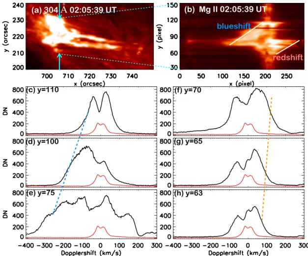
Over the course of the reconnection phase (starting at 02:04 UT) the MgII, CII, and SiIV spectra show extended blue and red wings around the pixel value of 80. As an example, we show MgII k line spectra (Fig.8b). At the pixel value 80, the MgII
line profile is the most extended one on the blue and red sides like in bidirectional outflows. This kind of bidirectional flow has been interpreted as being the site of reconnection in some events (Ruan et al. 2019). Therefore, we consider this zone (around the pixel value 80) to be the reconnection site.
Rapidly (in less than one minute), we see an extension of the brightening of the wings of MgII k spectra in pixels along the slit in the central zone (pixel value 60 to pixel value 120) (Fig.8a). In the north and south parts of the reconnection site, we note that the spectra shows a tilt. The Mg II profiles are not symmetrical all along the slits; they present some bilateral flows only in a few pixels around y= 79. Otherwise, they have extended blue wings for example for pixel y > 85 and not corre-sponding red wings. It is the reason that we do not consider that the bilateral flows exist all along the slit (10 Mm long). There-fore, the existence of this gradient and tilt is obvious. The tilt is characterised by the gradient of the Dopplershifts that exist for profiles along the slit at a given time. The line profiles of MgII kline show important extensions of the wings at 02:05:39 UT (Figs. 8c-h). They predominantly show an extended blue wing in the northern part (pixel value 75 to pixel value 110 (c-e)) with decreasing blueshifts at y= 110; they are roughly symmetric in the middle of the brightening (y= 80) with more extended blue wings nevertheless (until −300 km s−1). In the southern part of
the brightening, the profiles have a dominant enhancement in the red wing (pixel value 63 to pixel value 70 (f–h)). The x-axis of the Fig.8shows Dopplershifts in km s−1. These Dopplershifts do
350 km/s 80 km/s
100 km/s
30 km/s
40 km/s
(a) AIA 171 02:05:05 UT
Å
(b) AIA 171Å
(c) AIA 304
Å
(d) AIA 211Å
80 km/s
350 km/s
Fig. 6.Height-time profile for the jet in different AIA wavelengths (b-d). The location of the slit (width = 8 pixels) along the plasma flow direction,
which is used to generate the height-time plot, is shown as the white solid line in panel a. The jet and surge both showed a two phase eruption, i.e. fast and slow. The jet is erupted with a high speed of ≈350 km s−1and after that it is slowed down to ≈80 km s−1(panels b–c). The surge is erupted
with a maximum speed of ≈100 km s−1and the dense material came back to the source region with a speed of ≈40 km s−1(panel d).
not really correspond to up and down flows because the region is located at 60◦ in the west. Therefore, the blue-shifted
mate-rial is going, in fact, to the left of the reconnection site over the EMF2 and not in the direction of the jet. This means that all cool material visible at −300 km s−1for which the emission is
relatively high in the MgII wings is going to the east and the redshifted material is expelled toward the west side as is the jet, with a maximum velocity of 80 km s−1. The transverse velocity of the cool material along the west side has dispersed values of between 30 km s−1 and 100 km s−1. This means that one part of the cool red-shifted material could be nearly normal to the solar surface while the other part would be inclined like the jet. A similar behaviour is observed in the four positions of the slit for Mg II, C II, and Si IV lines (Fig.9). The tilt in the four Si IV spectra is even more readily visible because Si IV is a transi-tion region line with only one emission peak when compared to chromospheric lines with two peaks.
This type of tilt spectra along a slit was first observed for prominences (Rompolt 1975) and interpreted as rotating promi-nences before eruption. Thanks to the Solar Ultraviolet Measure-ments of Emitted Radiation (SUMER) spectrograph onboard SOHO, and now also with the IRIS spectrograph, such a tilt behaviour in the spectra is frequently observed. They are well-known and typically associated with twist (De Pontieu et al. 2014) or rotation (Curdt et al. 2012), or flows of plasma in heli-cal structures (Li et al. 2014). In Li et al.(2014), the long
fila-ment crossed by the IRIS slits changed the direction of its rota-tion in the middle of the filament. In our observarota-tions, the jet is rotating in the same direction in all four positions. The slit scanned only 6 arc sec of the jet, mainly capturing the jet base with the dome shape.
The tilt in our spectra finally reach a length around 60 pix-els, which represents around 15 Mm. We interpret this tilt by the rotation of a structure crossed by the slit, the structure being the base of the jet or, possibly, cool plasma that follows helical structures. The profiles of the MgII kline with extended wings resemble the profiles of the IRIS bombs (IBs) that were dis-covered by Peter et al.(2014) and analysed by Grubecka et al. (2016) andZhao et al.(2017).Grubecka et al.(2016) found that the IBs were formed in the very low atmosphere between 50 to 900 km in the chromosphere. The magnetic configuration of the reconnection site is similar to that of the Ellerman bombs (EBs) in BP regions, where there is no vertical magnetic field (Georgoulis et al. 2002; Zhao et al. 2017). We conjecture that between the two EMFs in the QSL region, there is a BP recon-nection region as in IBs (Zhao et al. 2017). The BP topology in the region of the present jet is confirmed in the topological anal-ysis (Sect.4). The cool material which is expelled towards the east could correspond to the dark blobs that previously existed in this area, which were trapped in the BP region while the BP was forming between two mini-flare events.
x
Fig. 7.Solar jet observed in co-aligned images of EUV AIA 304 Å (top), of IRIS C II SJI (middle), and of IRIS Mg II SJI (bottom). The four positions of the slit in the raster mode are shown with vertical cyan lines in panel g. The dark vertical line in each panel d–i is the footprint of one position of the slit during the SJI shooting. In IRIS CII SJI images (middle row), the reconnection point is indicated as “X” in panel d and the original observed pixel values along the y axis are displayed in panel e. The FOV of these panels is indicated in Fig.3a. In this figure we keep the nominal coordinates of IRIS which are translated by+4 arcsec in x and +3 in y compared to the AIA coordinates.
4. Magnetic topology of the jet region
In Sect.3.1.1, we follow the birth of the AR using HMI longi-tudinal magnetic field. Here, we analyse the magnetic topology of the AR using the full vector magnetic field to understand the orientation of the magnetic field lines inside the two bipoles (P1-N2 and JP1-J(P1-N2) involved in the mini-flare and the jet to confirm the existence of a BP.
4.1. HMI Magnetic field vector maps
The HMI SHARP longitudinal magnetic field movie, with its high cadence, shows the fast evolution of the EMF2. The nega-tive polarities N2-JN2 were continuously sliding along the pos-itive polarity P1 of EMF1 and initiating bright points from time to time. Therefore, we used the HMI vector magnetic field map at the closest time of the reconnection at 02:00 UT.
(a) 304 02:05:39 UT
Å
(b) Mg II 02:05:39 UT
(c) y=110 (d) y=100 (e) y=75 (f) y=70 (g) y=65 (h) y=63blueshift
redshift
Fig. 8.Mini-flare and the bright jet with two branches inserting a cool dense surge in AIA 304 Å (panel a). The cyan arrows show the location of the slit position 1. The Mg II k line spectra corresponding to the slit position 1 which is crossing the reconnection site is shown in panel b. The red and blue shift wings are shown by the white tilted lines on the left (blueshift) and right (redshift) in the spectra. The bottom rows (c– h) show the Mg II k line profiles for different y values using unit of velocity in the x axis. Panels c–e concern the blue shift profiles. shown by the tilted blue dashed line corresponding to strong blueshifts (−300 to −100 km s−1). Panels f–h show the red shift profiles. Redshifts (80–100 km s−1) are shown
by the red dashed tilted line. The red and blue dashed lines are passing through the inflexion points of the line profiles in panels c– h.
Figure10presents in the right panel the magnetic field vector map computed with the UNNOFIT inversion code at 02:00 UT and the corresponding full AR (left panel) as a contextual image meant to show the brightening at the base of the jet in AIA 94 Å. The vector magnetic field maps represent the full magnetic field vectors with their three components in the solar local reference frame, generally referred to as the heliospheric reference frame. The vertical component in this reference frame is represented via a colour table. The two horizontal components are associated to form an horizontal vector, which is represented by arrows. However, the pixel dimension is viewed along the line of sight in order to be able to co-align the FOV with the AIA images.
A box indicates the small FOV encircling the region which contains the brightening at the jet base corresponding to the QSL at the reconnection site. We carried out a zoom analysis to probe the nature of magnetic field vectors in this jet region (Fig.11a). The length of the arrows represent the strength of the horizon-tal magnetic field. We recognise the polarities identified in the longitudinal magnetic field map (Fig.11b).
4.1.1. Flux rope (FR) vector pattern
In the long region between P1 and N2, we make note of a char-acteristic pattern of the magnetic field vectors that suggests the
presence of a twisted FR with vectors converging together in the PIL in the middle part (between P1 and N2) and vectors turning at both ends, in the top and bottom parts of the FR, resembling the hooks of a FR (Fig.11a). In the vicinity of the FR, there is an interface that separates the regions of turning and returning of the vectors, which represent the boundary between the FR and the arcades over the FR and its surrounding area.
This pattern is relatively stable according with the 22 maps computed around the jet time. On 21 March at 20:00 UT, the FR was already created and was continuously observed until 22 March at 05:00 UT. At first glance, the FR does not seem to par-ticipate to the formation of the jet. A very detailed study shows that, in fact, this was a very particular case involving a transfer of twist from the FR to the jet during the FR extension towards the south before the reconnection. This is further explained in the next section.
4.1.2. Formation of the small bipole
The relationship of the FR and the jet is detected in the HMI movie of the longitudinal magnetic field where the formation of the small bipole (where the jet was initiated) is observed. The longitudinal HMI movie (animation attached as MOV1) shows a stress created by the sliding of the two opposite polarities
(a) 02:05:39
(e) 02:05:39
(i) 02:05:39
(b) 02:05:43
(c) 02:05:46
(d) 02:05:50
(f) 02:05:43
(j) 02:05:43
(g) 02:05:46
(h) 02:05:50
(k) 02:05:46
(l) 02:05:50
Mg II
Si IV
C II
Fig. 9.Tilt observed in the three lines Mg II (left column), C II (middle column), and Si IV (right column) observed with IRIS instrument. The four different rows are showing the spectras at the four different slit positions from east to west: 1, 2, 3, and 4.
(a) AIA 94 02:00 UT
Å
(b) 02:00 UTFig. 10.Panel a: jet base appearing as brightening with an arch-shape in between the positive (green contours) and negative (blue contours) in AIA 94 Å. Panel b: HMI Vector magnetic field map with the same FOV as of the (a). The white square is the FOV for the Figs.11a and b. The colour bar indicates the vertical magnetic field strength and the arrow on the right the strength of the horizontal magnetic field in the map in (b).
(P1 and N2). These two polarities come from the two opposite magnetic emerging regions (EMF1 and EMF2). On 21 March at 23:00 UT, a few hours before the jet, a negative polarity part
of N2 detaches and moves towards the south, sliding along the positive polarity P1 to form the small bipole JN2-JP1 (Figs.11g-j). The new bipole is formed with the small positive
(c) 21 March 23:00 UT (d) 22 March 00:12 UT (e) 22 March 02:00 UT (g) 21 March 23:00 UT (h) 22 March 00:12 UT (b) 22 March 02:00 UT (a) 22 March 02:00 UT (a) 22 March 02:00 UT (f) 22 March 02:12 UT (j) 22 March 02:12 UT (i) 22 March 02:00 UT (a) 22 March 02:00 UT N2 P1 JP1 JN2
Fig. 11.Panel a: vector magnetic field configuration of a part of AR NOAA 12736 where the jet is initiated. Panel b: LOS magnetic configuration at the AR including the two bipoles P1-N2, JP1-JP2. The FOV of panels a and b is presented as the red square in Fig.1e. Panels c–f: zoomed view of vector magnetic field configuration and panels g–j: zoom view of LOS magnetic field configuration at the small bipole location, where the magnetic flux cancellation occurs. The detached negative (black) polarity is moving towards the south and is shown with white arrows. The FOV of these panels is shown as the white square in panel b. On the left the colour bar indicates the vertical magnetic field strength and the arrow shows the strength of the horizontal magnetic field in the map (panel a and panels c–f).
(JP1) and the negative (JN2) polarity encircled in Fig.11e. This small bipole is formed by collision of two opposite sign polar-ities coming from two different magnetic systems and not by direct magnetic flux emergence.
4.1.3. Bald Patch (BP) magnetic configuration
Looking at the direction of the magnetic field vectors between JN2 and JP1, we find that they are oriented from the negative polarity to the positive polarity, which is evidence that it is a BP region, more generally, that it is a region with magnetic field lines that exhibit a dip grazing the surface at the PIL (Fig.11e). We note that the BP is observed only at this precise time (02:00 UT) – and not before and not after (Figs.11c, d, and f).
4.1.4. Transfer of twist
We arrive at the conclusion that with the extension of the FR towards the south, it is possible that the arcades of FR interact with the overlying magnetic field. Some part of the twist of the FR could be transferred to the jet, however, there is still a rem-nant component in the small bipole, as we see in Fig.11f. The rotation of the structure at the base could explain this transfer of twist. To make certain of the existence of the FR, we compare this finding with MHD simulations.
4.2. MHD Model
4.2.1. Description of the MHD simulation
We used the MHD simulations ofZuccarello et al.(2015), where the physical conditions are used to create a FR in an AR. Start-ing from an asymmetric, bipolar AR, as inAulanier et al.(2010), they investigated different classes of photospheric motions that are capable of forming a FR. Here, we consider the results of the simulations with regard to converging motions towards the PIL of the AR with magnetic flux cancellation. Progres-sively twisted magnetic field lines were globally wrapping around an axis and, eventually, formed a FR. The dynamics of the FR is modelled by using a version of the Observation-ally driven High-order scheme Magnetohydrodynamic (OHM) code (Aulanier et al. 2005,2010). It is a β= 0 simulation, so the plasma conditions are not studied. The MHD simulations have already been validated by testing different flare activities, such as sigmoid currents of FR (Aulanier et al. 2010), electric current density increase in flare ribbons (Janvier et al. 2014), and electric current density decrease at CME footpoints (Barczynski et al. 2020). In this study, we want to test if the footprints of the FR in the HMI magnetic vector (vec B) maps have a similar pattern as the footprints of the theoretical FR in these MHD simulations.
(a)
(c)
(d)
(b)
5.2 MHD space units 15 Mm -1200 Gauss-1.7 0.9 1.7 2.6Fig. 12.Flux rope (FR) evidenced in the HMI observations (a, b) and comparison with the images from MHD simulations (c, d). Panel a: vector magnetic field map computed with the UNNOFIT code and the yellow (dark) blue areas show the positive (negative) magnetic field polarity. Panel b: current density map computed with UNNOFIT code. The FOV for panels a-b is presented in Fig.11a and to compare with MHD simulation we rotated the observations 30◦
clockwise. Panel c: from MHD simulations the iso-contours of vertical magnetic field with vectors. The pattern of the green vectors is same as with the yellow vectors in observations in panel a. Panel d: the magnetic field lines are plotted with the grey colour and the red and blue contours are electric currents. So the FR has a very strong electric currents, with the current flowing from red to blue. The vector pattern of observations and model looks the same, as they are strongly nearly parallel to the PIL and converging together in the bottom part. The convergence is due to the asymmetry of the magnetic configuration. The colour bar (top left) indicates the vertical magnetic field strength in Gauss for panel a, the colour bar (top right) the strength of electric current in mA m−2for panel b, the colour bars (bottom right) represent the strength of
the electric current in MHD units (left colour bar), and in physical units (right colour bar) for panel d.
4.2.2. Comparison between MHD models and observations: FR pattern of vec B
The comparison between our observations (panels a-b) and MHD simulations (panels c-d) is presented in Fig.12. We rotated our observation in panels a-b by 30◦in the clockwise direction
for an improved comparison with the MHD simulations. It is very clear that a sheared magnetic field is generated along the
PIL and the vectors are strongly inclined along with PIL. We have also evidence for swirling of the magnetic field in the top and bottom part of the FR.
The sheared vec B that converges towards the PIL is a char-acteristic motion to create a BP. This pattern can also be seen inBarczynski et al.(2019). It is due to the summed effects of: (i) the shear that creates a BP with vec B in the negative polar-ity pointing towards the positive polarpolar-ity; and (ii) the asymmetry
P1 N2 JN2 PIL JP1
( a )
arcade flux rope JN2 P1 N2 JP1 PIL( b )
bald patch displacement ofbald patch current-sheet
JP1 P1 N2 PIL
( c )
X-point JN2 start of jet X-point current-sheet JP1 P1 N2 PIL( d )
JN2 untwisting jet shear remnantFig. 13.Sketch of the formation of the jet and transfer of the twist from the FR to the jet during reconnection. Panel a: magnetic configuration before the reconnection, panel b: formation of the BP current sheet, panel c: X-point current sheet, panel d: untwisting jet after the reconnection and the remnant twist in the bipole JP1 and JN2. The dashed lines represent the non-eruptive FR, the arcade between P1 and N2 (dashed line in (a)) reconnects at the BP with the dashed line on the right in (b) creating a long dashed field lines from P1 to the extreme right. Below the arcade, the twisted line P1-N2 of FR (solid line) is elongated in (b) and touches the BP region in (c), it reconnects with an open magnetic field line (solid line on the right in (c)) creating the untwisting jet in (d).
of the photospheric flux concentration with a stronger positive polarity (in the model and observations) which is due to the mag-netic pressure pushing all the fields towards the (weaker) nega-tive polarity. Hence it is leading to some sheared vector within the positive polarity to point towards the negative polarity. These two effects lead to the convergence.
The swirling motions visible at both ends of FR are well-represented by vec B, which display similar angles and simi-lar spatial gradients at the edges of the swirlings, which sep-arate the swirling vec B from the surrounding magnetic field that has more potential, that is, exhibiting more radial from the center of the magnetic polarity. For example, this separation is
visible at the top right in Fig.12a and c in the positive polarity, where radial vectors are close to turning vectors to the left, and at the bottom of the negative polarity, there is a similar separa-tion between radial vectors and vectors turning to the left. This kind of separation is reminiscent of a QSL, just as in the MHD models (Janvier et al. 2013;Aulanier & Dudík 2019). Moreover, those swirls correspond exactly to the footpoints of sigmoidal field lines, even though they are not visible in the extreme ultra-violet (EUV). Finally, the similarity of all these characteristics structures (e.g. BP, QSL, sigmoidal field line) between the MHD models and our observations leads us to infer the existence of a FR in the immediate vicinity of the jet.
4.2.3. Comparison between the MHD model and observations: electric current density (Jz) pattern
In addition to the pattern of the photospheric horizontal fields, a relatively good match is also found for the vertical current densi-ties. Both the HMI observation and the MHD simulation display a dominance of the Jzand Bzof the same signs in each
polar-ity of the bipole, with an elongated double-peaked Jzpattern all
along the PIL, as well as more extended patches at the ends of the sheared PIL.
In the model, those extended patches correspond to the foot-points of the FR field lines (Fig.12d). One difference, however, between the observation and the model is that with HMI, the extended patches in the negative polarity is more clearly visi-ble than in the positive polarity (see Fig.12b). We argue that this difference is minor since it may be due to that fact that in the pos-itive polarity, the swirling patterns of the vector fields are located in relatively weaker vertical fields than in the negative one (i.e. 500G in the former vs. 1500G in the later, see Fig.12a). With the same twist in both polarities, the weaker fields result in weaker current densities in the positive polarity. Another difference is that in the MHD simulation, some strong QSL-related current sheets surround the FR footpoint related extended patches (see Janvier et al. (2013), Aulanier & Dudík (2019). These are not visible with HMI and we argue that this is due to the limita-tions of the HMI data, from which current sheets can only be extracted during flares and with some processing of the data, as inJanvier et al.(2014),Barczynski et al.(2020).
4.2.4. Comparison between the MHD model and observations: magnitude of Jz
Comparing the magnitudes of current densities between mod-els and observations requires us to scale the model to physics (solar) units. The reason behind this is that the model was cal-culated with dimensionless units, resulting in maximum current densities on the order of five units. Such a scaling has already been done for the estimation of flare energies (Aulanier et al. 2012, 2013). Here, they need to be adjusted to this specific observed bipole. Still, we should bear in mind that this can only be done approximately given the differences in shape between the observed and modelled flux concentrations. Thus, using HMI as a reference (Fig.12a), we attributed a magnetic field ampli-tude of ±1200 G to the Bz isocontour Bz = ±1.7 and a bipole
size of 15 Mm to the width of 5.2 space units as displayed in Fig.12c. Then we scaled the OHM model using a magnetic unit B0= 7.1 × 10⁻²T and a spatial unit L0 = 2.9 × 10⁶m. We reset
the magnetic permeability from unity in the simulation to its real value µ= 4 π × 10−7 SI units. As a result, the dimensionless
current-densities that we model here have to be multiplied by B0/(µL0) to be expressed in A m−2. With these settings, the
cur-rents reached up to 100 mA m−2at the FR footpoints. This value is only half of what is measured with HMI, so the modelled cur-rents are in qualitative agreement with the observed ones. The difference in magnitude may be attributed to the existence of a stronger twist in the observed bipole than the twist in the model. Yet it is arguably more likely due the different aspect ratios of the observed and modelled bipoles, the latter being less elon-gated than the former (compare Figs.12a and c).
5. Discussion and conclusions
5.1. Summary of observations and methodology
The present study concerns multi wavelength observations of a jet and mini-flare occurring in the active region (AR) 12736 around 02:04 UT. We adopted a different methodology than the methodology ofYang et al.(2020), where the same flare activ-ity was analysed, which resulted in a difference of interpretation. We looked at the detail history of the polarities and vec B using HMI data instead of the Hinode data, covering the AR, half an hour before the jet. The activity was recurrent and evolved very fast with a chain of similar phases. Mini-flares in this AR were observed frequently changing the connectivity at this interface region from a bald patch (BP) region to a current sheet region and vice-versa. The main bipole (P1-N2) is the result of collision between two emerging fluxes. The negative polarity is sliding, extending towards the south, creating a small bipole (JP1-JN2) and it is cancelled out with the positive polarity. The history of the AR tells us that JN2 was detached from N2, generating a strong shear along JP1.
UnlikeYang et al.(2020), we did not make a NLFFF mag-netic extrapolation and, instead, we preferred to use the horizon-tal vector magnetic field (vec B) observations directly to relate the small bipole and the BP to the origin of the jet (both posi-tioned at the same place). We compared the observed magnetic field vec B pattern and the values of the electric current den-sity Jz with synthetic Jzand vec B data from the MHD model
of FR (Aulanier et al. 2010;Zuccarello et al. 2015) to infer the location of FR. The FR is identified between P1 and N2 in the HMI vec B maps. It is definitively not the FRs computed by the magnetic extrapolation ofYang et al. (2020) neither their first FR (FR1) between N2 and P2 (which, in fact, corresponds to an arch filament), nor their second FR (FR2), with NS field lines corresponding to a small filament not visible by absorp-tion in any AIA filters before the jet. The FR1 has one end in N2 like our FR but the second end is in P2. In our case, the second end (foot) of the FR is in P1, where we have the sig-nature of a hook in the vec B maps (HMI as well as in Hin-ode). No similar pattern exists in P2 in the vec B maps. Our detailed observation analyses suggest that the jet reconnection occurred in a BP current sheet and in the, rapidly formed above null (“X”) point, current sheet, driven by the moving polarity (JN2) that carried twist from the remote FR and injected it into the jet. The initial FR remains stable during the reconnection process.
5.2. Scenario of transfer of twist (cartoon)
We proposed a cartoon where the FR between P1 and N2 is rep-resented by the solid twisted line (Fig.13a). It is extended to the south, creating the bipole JN2-JP1. The BP current sheet is gen-erated between the overlying arcade of FR and the magnetic field line of the west emerging flux P1-N1 (panel b). At this time, a first reconnection occurs at a localised point that is very deep in
the atmosphere. The Mg II profiles resemble those found in IRIS bombs (IB) with extended wings (Peter et al. 2014), which are proposed to have been formed during BP current sheet reconnec-tion (Zhao et al. 2017). Such chromospheric wide profiles have been modelled in MHD simulations (Hansteen et al. 2019). It has also been shown that a BP could be transformed immedi-ately at a null point. We propose in panel c that the reconnection occurs in the null point (“X”-point) that is formed dynamically along a current sheet or a flat spine-surface above a dome that is not depicted in the cartoon panel c. Cool material trapped in the BP during its formation is expelled with a large blueshift, as revealed in IRIS Mg II line profiles with extended blue wings. The spectra shows an evident tilt, which indicates the presence of helical motions. The reconnection site is heated at all the temper-atures and the hot jet is expelled towards the west side in twisted field lines (panel d). The cool material follows different paths than the hot and acts as a wall in front of the hot jet. It resem-bles the surges that accompany jets in the MHD simulations of Moreno-Insertis et al.(2008),Nóbrega-Siverio et al.(2016), and Nóbrega-Siverio et al.(2018). The HMI vec B map shows some remnant twist in the bipole JP1 and JN2 after the ejection (panel d), which offers evidence that the twist has gone mainly into the ejected jet.
5.3. Scenario of the breakout
The scenario proposed by Yang et al. (2020) is based on their own NLFFF magnetic extrapolation, which suggests that the small FR2 erupted in the breakout scenario with a reconnection at a null point (Antiochos & DeVore 1999). We agree globally to the NLFFF extrapolation with the existence of a null point, fan, and spine. The QSLs are well defined and could correspond to the base of the dome as we describe as QSLs are robust struc-tures but their precise location is difficult to determine accu-rately and to thus serve as an argument for localising filaments (Dalmasse et al. 2015;Joshi et al. 2019).
The role of FR2 is important in their case, with its strong pre-existing shear. They argue that it is an instability breakout-related jet leading to a full evacuation of their FR2 (Sterling et al. 2016; Wyper et al. 2017). However, the identification of their FRs in the observations is difficult in AIA images, where there are mixed bright and dark paths in this zone (Fig.7), and even in the images of NVST. In addition, the ejection of the cool mate-rial is blue-shifted, so it runs in the opposite direction to the hot jet. It is difficult to trust that the eruption of this cool material is the driver of the jet.
Moreover, in their NLFFF magnetic extrapolation the null point is located quite far from the tiny bipole JN2-JP1 (see Fig. 3 in their paper), which is, hence, far from the observed origin of the jet. This location of the X point is may be due to the fact that the authors worked with an earlier vect B map from nearly half an hour before the reconnection. It could be the location of the former X point of the previous mini-flare, which is when JN2 was not yet colliding with JP1. The BP was not yet formed at this early stage. We show that it is important to take into account the history of this AR, which evolved quite fast. This difference in the localisation of the null point could be due to the nonalign-ment of HMI, AIA, and IRIS images in the paper ofYang et al. (2020), where the authors do not note that the nominal coor-dinates of these instruments have 4 arcsec in x, 3 arcsec of y difference and, instead, they mention a projection effect. 5.4. Conclusions
In this paper, we present the observations of a twisted jet, a surge, and a mini-flare which occurred in the active region
(AR) 12736 on 22 March 2019 at 02:05UT. The event was observed in multi-wavelengths with AIA and IRIS instruments and detailed in the magnetic field vector maps obtained by HMI and computed with the UNNOFIT code. The MHD simulations were used to validate the vec B observations (Aulanier et al. 2010;Zuccarello et al. 2015). We present our main results in the following :
1. The AR consisted of the collapse of two emerging magnetic flux (EMF) regions, each of them overlaid by an arch fil-ament system (AFS). The jet and surge reconnection site is along the PIL between these two AFS. The AFS over the east side evolved rapidly due to photospheric surface motions. Prior to the reconnection, the AFS exhibit a dome shape. After the reconnection, long AFS overlying both EMFs are observed. This is confirmed in the NVST Hα images. 2. A large flux rope (FR) in the vicinity of the jet region is
detected. The patterns of transverse fields and vertical cur-rent densities, as observed by HMI and appearing with-out being constrained a priori in an MHD simulation of non-eruptive FR formation with flux-cancellation of sheared loops, show a good accordance. The location of the FR is fully supported by HMI vec B and electric currents Jzmaps.
3. The magnetic topology of the AR demonstrates a bald patch (BP) region due to the particular formation of the bipole by collision of opposite polarities, which is dynamically trans-formed to an “X”-point current sheet.
4. The fast extension of the FR towards the site of reconnection due to photospheric surface motions offers the possibility for the FR arcades to reconnect with magnetic pre-existing field lines at the “X”-point current sheet without the eruption of the FR. The extension of the FR may transmit twist to the jet.
5. The IRIS spectra at the reconnection site display a tilt and gradient in the spectra along the jet base, indicating the for-mation of a rotating structure during the reconnection. The clues leading to our interpretation consists of the identifi-cation of a non-eruptive FR, from which some twist is carried away and eventually reconnected into the jet at the “X”-point current-sheet. The transport of twist away from the FR towards a BP is supported by the HMI observations of a moving negative flux-concentration whose transverse fields point towards a pos-itive one. The twist is transported at a long distance of the FR which remains non-eruptive. The tilt observed in the IRIS spec-tra in the four positions of the slit, which, by chance, are exactly at the site reconnection, confirms the transfer of twist at the jet base.
Our magnetic analysis benefit from the treatment of the HMI vec B by the UNNOFIT code, which uses a filling factor that takes into account the non-resolved structures. In each pixel, there is an equilibrium between magnetised regions and non-magnetised regions, which implies a better determination of the magnetic field inclination (Bommier 2016). This is an impor-tant aspect for regions with a weak magnetic field. This is the case in the small bipole, where our jet reconnection takes place and where we have detected the BP. The second aspect that is important in this study is the chance to have the IRIS spectra at the right place, namely, at the reconnection site. The IRIS spectra directly shows the transfer of twist between two sta-ble systems at the reconnection point by unveiling a helical structure.
Observations of bright jets simultaneously followed with cool and dense material or surges are an interesting area of study to probe by spectroscopic analysis using the IRIS instrument. The IRIS spectral profiles are very useful tools for explaining