HAL Id: hal-01421817
https://hal.archives-ouvertes.fr/hal-01421817
Submitted on 3 Feb 2017
HAL is a multi-disciplinary open access archive for the deposit and dissemination of sci-entific research documents, whether they are pub-lished or not. The documents may come from teaching and research institutions in France or abroad, or from public or private research centers.
L’archive ouverte pluridisciplinaire HAL, est destinée au dépôt et à la diffusion de documents scientifiques de niveau recherche, publiés ou non, émanant des établissements d’enseignement et de recherche français ou étrangers, des laboratoires publics ou privés.
Shale dynamic properties and anisotropy under triaxial
loading
Joël Sarout, Laurent Molez, Yves Guéguen, Nasser Hoteit
To cite this version:
Joël Sarout, Laurent Molez, Yves Guéguen, Nasser Hoteit. Shale dynamic properties and anisotropy under triaxial loading. Poromechanics III - Biot Centennial (1905-2005), May 2005, Norman, Okla-homa, United States. �10.1201/NOE0415380416.ch94�. �hal-01421817�
Shale Dynamic Properties & Anisotropy under Triaxial Loading
Jo¨el Sarout, Laurent Molez Yves Gu´eguen
Laboratoire de G´eologie, Ecole Normale Sup´erieure, Paris, France.
Nasser Hoteit
Agence Nationale pour la gestion des D´echets RAdioactifs, France.
This paper is concerned with the experimental identification of the whole dynamic elastic stiffness tensor of a transversely isotropic clayrock from a single cylindrical sample under loading. Measurement of elastic wave velocities (pulse at 1 MHz), obtained under macroscopically undrained triaxial loading conditions are provided. Further interpretation of the velocity measurements is performed in terms of (i) dynamic elastic parameters ; and (ii) elastic anisotropy. A discussion concerning microcracks and fluid content (saturation) issues follows. Experiments were performed on a Callovo-Oxfordian shale, Jurassic in age, recovered from a depth of 613 m in the eastern part of Paris basin in France.
1 INTRODUCTION
1.1 Callovo-Oxfordian Shale
Clayrocks, and shales in particular, represent approx-imately two-third of all sedimentary rocks. In oil and gas drilling operations, shales constitute 80 % of all the drilled sections, mainly because they overlie most hydrocarbon bearing reservoirs. Furthermore, several countries are considering clayrocks as pos-sible host lithologies for radioactive waste confine-ment, and therefore carrying out research programs to estimate feasibility of such solution. In this trend, the french agency for radioactive waste management, ANDRA, is evaluating the reliability of the Callovo-Oxfordian layer, Jurassic in age, located in the eastern part of France (Bure), at a depth ranging from 400 m to 700 m. The static mechanical properties of this clayrock have been largely studied for the past few years (complete bibliography in Escoffier (2001)). However, very few velocity measurements, all at at-mospheric pressure, were performed, and no veloc-ity data at all under mechanical loading are avail-able in the literature for this rock. The main out-come of interest here from these research programs is the transversely isotropic nature of Bure clayrock demonstrated experimentally in several labs for sev-eral locations and depths in the layer (David 2004). The main plane of symmetry is quasi-horizontal and corresponds to a very fine layering (bedding). This clayrock is then called a shale in the following.
1.2 Shale Lithologies
In general, the monitoring of elastic velocities in shales under mechanical loading are relatively un-common in view of the abundance of this lithology in the shallow earth crustal rocks (Stanley and Chris-tensen 2001). This relative rareness is partly due to: (i) the inherent difficulty of transmitting transducer signals through the waterproof pressure chamber in a loading apparatus ; and, on the other hand, (ii) the specificities in preparing and handling shale samples for mechanical testing (chemical sensitivity to wa-ter, extremely low permeability...). Most of the dy-namic experimental studies reported in the literature on shale samples were performed under hydrostatic loading conditions (Johnston and Toks¨oz 1980; Jones and Wang 1981; Lo et al. 1986; Johnston and Chris-tensen 1995; Hornby 1998; Stanley and ChrisChris-tensen 2001). Only Yin (1992) carried out triaxial tests.
1.3 Main Goals
The specific experimental setup available in our lab allows for the simultaneous measurement of five dif-ferent velocities and two directions of strains on the same sample, under triaxial and pore pressucontrolled conditions of loading. This procedure re-duces the number of experiments on differently ori-ented samples usually needed to identify the dynamic properties of a rock. It also minimizes the errors due to the particular difference between two samples of
the supposedly same lithology or in the same physi-cal state (stress and saturation history since recovery from 613 m deep).
The main outcomes of this experiment are : (i) identification of the apparent dynamic stiffness tensor of the Callovo-Oxfordian shale from elastic velocity measurements ; (ii) assessment of velocity anisotropy, and its evolution under triaxial loading. This last step allows for the quantification of the intrinsic and stress-induced anisotropies, leading eventually to an estima-tion of the microcracks density and distribuestima-tion evolu-tions in the shale sample under loading (Vernik 1994). In the specific experiment described here, there are no strain data available during the hydrostatic load-ing because of experimental difficulties in strain gages gluing. However, an external LVDT allows for the es-timation of the sample global axial strain during the deviatoric loading.
2 EXPERIMENTAL PROCEDURE
2.1 Experimental Setup
The rock physics group in the geology laboratory of the Ecole Normale Sup´erieure recently acquired a tri-axial cell designed for the exploration of the hydrome-chanical behavior of shallow earth crustal rocks. This apparatus allows for pore pressure, hydrostatic and deviatoric stress to be applied independently on a cylindrical porous rock sample (up to ∅ 40 mm ×
L 80 mm). The pore, confining and axial pressures
may reach 100, 300 and 800 MPa (on the largest sam-ples), respectively. The originality of this loading cell is to allow for a maximum of 32 waterproof signal wires through the wall of the pressure chamber. The control and data acquisition are performed by means of a dedicated software designed in LabviewTM envi-ronment. The lab is temperature-controlled with an accuracy of ± 0.5◦C.
2.2 Sample Description and Preparation
The tested shale was provided by the french agency for radioactive waste management, ANDRA. The ceived large cores (∅ 90 mm × L 280 mm) were re-covered in 1995 from a depth of 613 m in the eastern part of Paris basin, near Bure, in France. These cores were since preserved in a so-called T1 cell, isolated from gas exchange with the storing environment, and maintained under small confining stress (. 1 MPa). The samples are dry-cored perpendicularly to the hor-izontal bedding, ground for parallel end faces, and preserved in waterproof membranes. In this specific experiment, the sample is 60 mm long with a 30 mm diameter. Few days before testing, during the phase of transducers gluing and curing on the sample, this one is maintained in a 100% relative humidity (RH) environment in order to avoid drying. Usually, af-ter putting it in 100%RH atmosphere, the mass of the
S-Polarization Propagation P-transducer S-transducer x1 x2 x3 VP ⊥ VSV VP || VP 45 VSH
Figure 1: Piezoelectric transducers arrangement and veloc-ity measurements on the shale sample.
sample increases then stabilizes. However, it is as-sumed that the sample may still be superficially unsat-urated. It is tested under macroscopically undrained conditions within the loading cell.
2.3 Transducers Arrangement
For the experiment reported here, 22 signal wires were used. Both axial and circumferential strain gages and nine piezoelectric transducers were glued on the cylindrical sample. However, the strain gages signals are rapidly lost at the beginning of the test. The specific arrangement of piezoelectric transduc-ers allows for the measurement of five different elas-tic velocities as shown in figure 1. Indeed, let us define the reference frame (x1, x2, x3), with (x1, x2)
being the horizontal bedding plane of symmetry of the transversely isotropic cylindrical shale sample. Then, measurements of three compressional veloci-ties and two shear velociveloci-ties, in three different direc-tions are provided. These velocities are referenced with respect to the bedding plane, i.e., VP(0◦) for the
bedding-parallel compressional velocity, VP(45◦) for
the 45◦-to-bedding compressional velocity, VP(90◦)
for the bedding-perpendicular compressional veloc-ity, VSH(0◦) for the horizontally polarized,
bedding-parallel shear velocity, and VSV(0◦) for the vertically
polarized, bedding-parallel shear velocity. In the case of transverse anisotropy, this latter is equal to the shear wave velocity VS(90◦) perpendicular to the
bed-ding. Note that the specifically designed compres-sional piezoelectric transducers are virtually load in-sensitive. On the other hand, the shear piezoceramics are simply glued to a fitting metal piece, itself glued on the sample, and are therefore load sensitive.
2.4 Measurement Technique
For velocity measurement, the classical Ultrasonic Pulse Transmission technique is used (Birch 1960; Tosaya 1982; Yin 1992). This method consists in measuring the travel time of a solitary elastic pulse through the rock sample of known travelling wave path length. The frequency of the solitary pulse in this experiment is 1 MHz.
2.5 Test Conditions & Loading Path
The chemical sensitivity of this shale to external wa-ter and its very low permeability precluded any pore pressure control of the test. Therefore, the tests are performed in macroscopically undrained conditions within the loading cell. The in-situ stress is estimated from depth and rock density. Indeed, we assume hy-drostatic state of stress in this large sedimentary basin, neglecting any deviatoric stress possibly due to tec-tonic stress build-up. This in-situ stress is estimated around 15 MPa.
The loading starts with confining pressure cycle between 0 and 55 MPa, i.e., (i) loading from 0 to 20 MPa ; (ii) unloading from 20 to 3 MPa ; (iii) re-loading from 3 to 55 MPa ; then (iv) unre-loading from 55 to 15 MPa. The loading rate is 0.013 MPa/s dur-ing the pressure-controlled hydrostatic loaddur-ing. After the fourth stage, a deviatoric stress is applied and in-creased until sample rupture. The deviatoric loading is displacement-controlled in order to avoid sudden sample failure. The velocity measurements are made after stabilization of all sample parameters at a given loading stage.
3 EXPERIMENTAL RESULTS
3.1 Error Analysis
For this particular experiment, corrections due to the rock deformation in the estimation of the velocity change during the hydrostatic loading are not feasible with accuracy because of a lack of strain measure-ment. However, a previous experiment on a similar sample, under the same conditions, allowed for strain data acquisition. Therefore, in the hydrostatic part of the present experiment, these strain data are used to correct velocity data. Both samples where cored ex-actly at the same depth, one centimeter far from each other, and no apparent heterogeneity was noted.
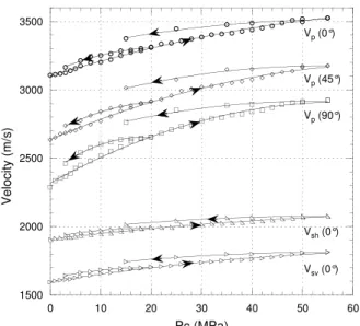
Furthermore, a complete error analysis of the Ultra-sonic Pulse Transmission technique has been carried out Yin (1992) and Hornby (1998). This analysis in-cludes the errors in the travel time picks for the mea-sured and reference travel times, and the error in the sample size measurements. In our experimental case, using Hornby (1998) equation (6), the relative error reaches a maximum of 1.1 % in the velocity measure-ments, depending on the wave type and propagation direction. 1500 2000 2500 3000 3500 0 10 20 30 40 50 60 Pc (MPa) V e lo ci ty (m /s) Vsv (0°) Vsh (0°) Vp (90°) Vp (45°) Vp (0°)
Figure 2: Elastic wave velocities evolution under hydro-static loading. 0 10 20 30 40 50 60 0 0.5 1 1.5 2 2.5 3 3.5 Axial deformation (%) D e vi a to ri c st re ss (M P a )
Figure 3: Axial stress – axial strain curve.
1500 2000 2500 3000 3500 0 0.5 1 1.5 2 2.5 3 3.5 Axial deformation (%) V e lo ci ty (m /s) Vsv (0°) Vsh (0°) Vp (90°) Vp (45°) Vp (0°)
Figure 4: Elastic wave velocities evolution under devia-toric loading, at 15 MPa confining pressure.
3.2 Experimental Data
Figure 2 shows the evolution of the five measured velocities VP(0◦), VP(45◦), VP(90◦), VSH(0◦) and
VSV(0◦), under confining pressure varying between
0 and 55 MPa. All velocities increase with increas-ing pressure, and a hysteresis effect exists upon pres-sure release at 20 and 55 MPa. Note that in the 0 −
55 MPa pressure range, ∆pVP(0◦) < ∆pVP(45◦) <
∆pVP(90◦). Even the amplitudes of the
hystere-sis velocity lags are ordered in the same way, i.e.,
∆hVP(0◦) < ∆hVP(45◦) < ∆hVP(90◦).
Figure 3 shows the axial stress-axial strain curve during the deviatoric part of the loading path. The sample failure happened probably around the peak ax-ial stress (51 MPa), and for a 1.9 % axax-ial strain.
Figure 4 shows the evolution of the five measured velocities VP(0◦), VP(45◦), VP(90◦), VSH(0◦) and
VSV(0◦), under this deviatoric loading. All velocities
decrease with increasing axial stress except VP(0◦)
which first increases until 1.3 % axial strain, then re-duces slightly.
4 THEORETICAL CONSIDERATIONS
4.1 Dynamic Stiffness Matrix
4.1.1 Definition
Transversely isotropic materials (hexagonal symme-try) may be adequately described in the elastic regime by five independent stiffness constants relating stress to strain components. They form a fourth order tensor which may be written in the Voigt notation as a twelve components matrix in the reference frame (x1, x2, x3),
i.e., C11 C12 C13 0 0 0 C12 C11 C13 0 0 0 C13 C13 C33 0 0 0 0 0 0 C44 0 0 0 0 0 0 C44 0 0 0 0 0 0 C66 , (1) where C12= C11− 2C66.
When evaluated from elastic wave velocity mea-surements, this tensor characterizes the dynamic ap-parent behavior of the material. These five indepen-dent Cij constants may be related uniquely to the five
classical Young’s, Poisson’s and shear dynamic mod-uli, i.e., E1d, E3d, ν12d , ν13d and µd13for instance.
These five independent Cij constants are related to
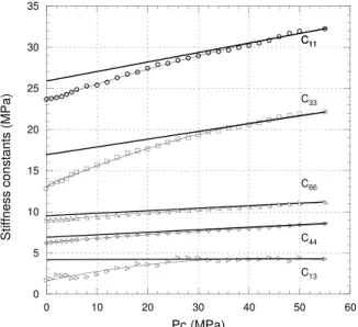
the five elastic wave velocities measured experimen-tally as follows : 0 5 10 15 20 25 30 35 0 10 20 30 40 50 60 Pc (MPa) S ti ff n e ss co n st a n ts (M P a ) C11 C13 C11 C33 C66 C44
Figure 5: Dynamic stiffness parameters evolution under hydrostatic loading. 0 5 10 15 20 25 30 35 0 0.5 1 1.5 2 2.5 3 3.5 Axial deformation (%) S ti ff n e ss co n st a n ts (M P a ) C13 C11 C33 C66 C44
Figure 6: Dynamic stiffness parameters evolution under deviatoric loading, at 15 MPa confining pressure.
C11 = ρVP2(0◦), C33= ρVP2(90◦),
C44 = ρVSV2 (0◦), C66= ρVSH2 (0◦), (2)
C13 = −C44+ [(C11+ C44− 2ρVP2(45◦))
(C33+ C44− 2ρVP2(45◦))]1/2.
4.1.2 Evolution under Loading
Figure 5 and 6 illustrate the evolution of the dy-namic stiffness parameters Cijwith increasing
confin-ing pressure and axial stress, respectively. Note that figure 5 allows for the estimation of the crack-free dy-namic moduli at low pressure.
0 0.1 0.2 0.3 0.4 0.5 0 10 20 30 40 50 60 Pc (MPa) A n iso tr o p y p a ra m e te rs γ ε δ
Figure 7: Anisotropy parameters evolution under hydro-static loading.
4.2 Anisotropy Parameters
4.2.1 Definition
In the specific context of transverse isotropy analysis, it is convenient to express three of the five dynamic elastic constants in (1) in terms of three anisotropy parameters, initially introduced by Thomsen (1986), i.e., ε = C11− C33 2 C33 , γ = C66− C44 2 C44 , δ = (C13+ C44) 2− (C 33− C44)2 2 C33 (C33− C44) . (3)
where ε measures the P-wave anisotropy, γ measures the S-wave anisotropy and δ is totally independent of horizontal velocity and may be either positive or nega-tive for geomaterials (Thomsen 1986; Hornby 1998). The main advantage of these parameters is their di-mensionless nature, therefore facilitating qualitative insight into the material behavior.
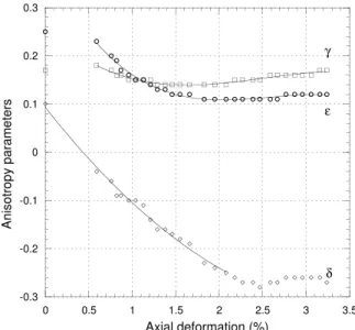
4.2.2 Evolution under Loading
Figure 7 and 8 show the evolution of velocity anisotropy parameters ε, γ and δ under hydrostatic and deviatoric loadings, respectively. Note the con-stant value of δ under hydrostatic loading and its dras-tic decrease until 2.25 % axial strain and then stabi-lization at a negative value under deviatoric load.
5 PHYSICAL INTERPRETATION: DISCUSSION
5.1 Anisotropy Issue
The main factors contributing to velocity anisotropy of rocks are: (i) preferred orientation of void space (pores and cracks) ; (ii) textural-structural features (bedding or foliation) ; and (iii) anisotropic con-stituent minerals. Crack-induced anisotropy reduces
-0.3 -0.2 -0.1 0 0.1 0.2 0.3 0 0.5 1 1.5 2 2.5 3 3.5 Axial deformation (%) A n iso tr o p y p a ra m e te rs ε γ δ
Figure 8: Anisotropy parameters evolution under devia-toric loading, at 15 MPa confining pressure.
with increasing hydrostatic load, leading eventually to the estimation of the intrinsic anisotropy at high con-fining pressure, due to factors (ii) and (iii) only. If we assume that crack-induced (subscript c) and intrinsic (subscript i) anisotropies are additive (Vernik and Liu 1997), we may extract the intrinsic anisotropies εiand
γifrom Fig. 7 at 55 MPa, i.e.,
εi = 0.23,
γi = 0.16. (4)
This allows for the estimation of the crack-induced anisotropy variation under hydrostatic loading, i.e.,
∆pεc= 0.19 and ∆pγc= 0.05. The δ parameter seems
constant under hydrostatic loading, i.e., δ ' 0.08. However, it is very sensitive to the deviatoric load, and decreases drastically with the increase of this lat-ter to a value of δc = −0.28 (Fig.8). Furthermore,
under deviatoric loading, both ε and γ anisotropy pa-rameters decrease until 1.3 % axial strain, then stabi-lize at εd = 0.11 and γd = 0.14. After, 1.9 % axial
strain, γ increases back. We therefore deduce that after closing the bedding-parallel microcracks under confining pressure, the deviatoric loading induces a damage to which the horizontal S-velocities are sen-sitive through the γ parameter. This damage may fur-ther be interpreted in terms of bedding-perpendicular microcracks. Note that for ε parameter, the crack-induced and intrinsic anisotropies are of the same or-der of magnitude, which confirms the importance of charaterizing the microcracked state of shales through anisotropy analysis.
The global analysis of the anisotropy data leads to a conceptual modeling of the microcracking history of a shale after coring and recovery. In general, (i) stress relief, (ii) microhydraulic fracturing, (iii) bot-tomhole stressing, (iv) dessication, and (v) in-situ
mi-crocracks, contribute to the final state of microcrack-ing in a rock sample in the lab. For this shale, microc-racks close under confining pressure, preferentially in the direction perpendicular to the bedding (bedding-parallel microcracks). The deviatoric loading induces damage (bedding-perpendicular microcracks).
5.2 Fluid Content and Saturation Issue
As pointed out by Jones and Wang (1981), the par-tial saturation of the sample manifests itself by the velocity hysteresis under cyclic confining pressure. They noticed that this hysteresis is drastically reduced when the shale sample is rehumidified, and even can-cels at very high confining pressure (400 MPa). In-deed, at ambient pressure, the void space is partially gas-saturated, in particular at the boundaries of the sample where gas exchange with atmosphere may oc-cur (surface drying). When submitted to a hydrostatic load, the microcracks closure reduces the void space, which is eventually totally occupied by the pore water at very high confining pressure. At this stage, hystere-sis due to partial fluid saturation is observable. In our experiment, it seems that even at 55 MPa confining pressure, hysteresis still exists, which allows us to as-sume that even at this pressure value, the pore space is still not fully saturated by water.
This brings out the question of effective pressure in the sample under loading. We will assume that dur-ing the hydrostatic loaddur-ing, the confindur-ing pressure is equal to the effective pressure, since the pore space is not water-saturated and the incompressibility of gas is negligible compared to that of liquid. The sample acts as under drained conditions.
Two other phenomena related to solid/fluid interac-tions are likely to occur in shales: (i) chemical soften-ing as a result of fluid-clay interaction and swellsoften-ing (smectites in particular) ; and (ii) physicochemical softening due to lubrication of grain interfaces. These issues are responsible for the inherent difficulty of shale experimental testing.
6 CONCLUDING REMARKS
Anisotropic elastic properties of a quasi-saturated Jurassic shale under macroscopically undrained con-ditions were determined by means of ultrasonic veloc-ity measurements. These five velocveloc-ity measurements were performed on the sample while under hydro-static and deviatoric loadings in a triaxial cell. The experimental method is based on a single core test, minimizing the errors due to the particular difference between two samples of the supposedly same lithol-ogy or in the same physical state (stress and saturation history since recovery).
Analysis and quantification of anisotropy may lead to the estimation of critical parameters such as micro-cracks density and orientation, as well as crack aspect
ratio, using Hudson’s or Kachanov’s models. This type of experiment will provide with input parame-ters for modeling wave propagation in porous, fluid-infiltrated, very low permeability shales. A natural way to model such medium is to use Biot’s dynamic theory of poroelasticity, possibly extended to account for squirt-flow phenomenon due to the existence of an equant porosity connected to an anisotropic one (crack-shape).
7 ACKNOWLEDGEMENTS
Support and shale samples for this research program have been provided by the french agency for radioac-tive waste management, ANDRA. This support is gratefully acknowledged. I would also like to thank Guy Marolleau for his crucial help in the setting of the experiment in the triaxial cell.
REFERENCES
Birch, F. (1960). The velocity of compressional waves in rocks to 10 kilobars. J. Geophys. Res. 65, 1083–1102. David, C. (2004). Personal Communication.
Escoffier, S. (2001). Caract´erisation Exp´erimentale du
Comportement Hydrom´ecanique des Argilites de Meuse/Haute-Marne. Ph. D. thesis, Institut National
Polytechnique de Lorraine, Nancy, France.
Hornby, B. E. (1998). Experimental laboratory determination of the dynamic elastic properties of wet, drained shales.
J. Geophys. Res. 103(B12), 29945–29964.
Johnston, D. H. and M. N. Toks¨oz (1980). Ultrasonic P and S wave attenuation in dry and saturated rocks under pres-sure. J. Geophys. Res. 85(B2), 925–936.
Johnston, J. E. and N. I. Christensen (1995). Seismic anisotropy of shales. J. Geophys. Res. 100(B4), 5991– 6003.
Jones, L. E. A. and H. F. Wang (1981). Ultrasonic veloci-ties in cretaceous shales from the williston basin.
Geo-physics 46(3), 288–297.
Lo, T.-W., K. B. Coyner, and M. N. Toks¨oz (1986). Ex-perimental determination of elastic anisotropy of berea sandstone, chicopee shale, and chelmsford granite.
Geo-physics 51(1), 164–171.
Stanley, D. and N. I. Christensen (2001). Attenuation anisotropy in shale at elevated confining pressures. Int.
J. Rock Mech. Min. Sci. 38, 1047–1056.
Thomsen, L. (1986). Weak elastic anisotropy.
Geo-physics 51(10), 1954–1966.
Tosaya, C. A. (1982). Acoustical Properties of Clay-Bearing
Rocks. Ph. D. thesis, Stanford University, Stanford, USA.
Vernik, L. (1994). Hydrocarbon-generaion-induced microc-racking of source rocks. Geophysics 59(4), 555–563. Vernik, L. and X. Liu (1997). Velocity anisotropy in shales:
A petrophysical study. Geophysics 62(2), 521–532. Yin, H. (1992). Acoustic Velocity and Attenuation of
Rocks: Isotropy, Intrinsic Anisotropy, and Stress Induced Anisotropy. Ph. D. thesis, Stanford University, Stanford,