HAL Id: hal-02453875
https://hal.archives-ouvertes.fr/hal-02453875
Submitted on 21 Aug 2020
HAL is a multi-disciplinary open access
archive for the deposit and dissemination of
sci-entific research documents, whether they are
pub-lished or not. The documents may come from
teaching and research institutions in France or
abroad, or from public or private research centers.
L’archive ouverte pluridisciplinaire HAL, est
destinée au dépôt et à la diffusion de documents
scientifiques de niveau recherche, publiés ou non,
émanant des établissements d’enseignement et de
recherche français ou étrangers, des laboratoires
publics ou privés.
C. Hibert, A. Mangeney, Gilles Grandjean, C. Baillard, D. Rivet, N. Shapiro,
C. Satriano, A. Maggi, P. Boissier, V. Ferrazzini, et al.
To cite this version:
C. Hibert, A. Mangeney, Gilles Grandjean, C. Baillard, D. Rivet, et al.. Automated identification,
location, and volume estimation of rockfalls at Piton de la Fournaise volcano. Journal of
Geo-physical Research: Earth Surface, American GeoGeo-physical Union/Wiley, 2014, 119 (5), pp.1082-1105.
�10.1002/2013JF002970�. �hal-02453875�
RESEARCH ARTICLE
10.1002/2013JF002970
Key Points:
• New seismology-based method for the identification of rockfalls • New method for the picking of the
rockfall seismic signals emergent onsets
• New seismology-based method for the location of rockfalls
Correspondence to:
C. Hibert, hibert@ipgp.fr
Citation:
Hibert, C., et al. (2014), Automated identification, location, and volume estimation of rockfalls at Piton de la Fournaise volcano, J. Geophys. Res. Earth Surf., 119, 1082–1105, doi:10.1002/2013JF002970.
Received 6 SEP 2013 Accepted 23 MAR 2014
Accepted article online 28 MAR 2014 Published online 15 MAY 2014
Automated identification, location, and volume estimation
of rockfalls at Piton de la Fournaise volcano
C. Hibert1,2,3, A. Mangeney1,4, G. Grandjean2, C. Baillard1, D. Rivet1, N. M. Shapiro1, C. Satriano1, A. Maggi5, P. Boissier6, V. Ferrazzini6, and W. Crawford1
1Institut de Physique du Globe de Paris, Paris, Sorbone Paris Cité, Université Paris Diderot, UMR 7154 CNRS, Paris, France, 2Bureau des Recherches Géologiques et Minières, DRP/RIG, Orléans, France,3Now at Lamont-Doherty Earth Observatory,
Columbia University, Palisades, New York, USA,4ANGE team, INRIA, CETMEF, Lab. J. Louis Lions, Paris, France,5Ecole et
Observatoire des Sciences de la Terre, Strasbourg, France,6Observatoire Volcanologique du Piton de la Fournaise/Institut
de Physique du Globe de Paris, Sorbone Paris Cité, La Plaine des Cafres, Réunion, Paris, France
Abstract
Since the collapse of the Dolomieu crater floor at Piton de la Fournaise Volcano (la Réunion) in 2007, hundreds of seismic signals generated by rockfalls have been recorded daily at the Observatoire Volcanologique du Piton de la Fournaise (OVPF). To study rockfall activity over a long period of time, automated methods are required to process the available continuous seismic records. We present a set of automated methods designed to identify, locate, and estimate the volume of rockfalls from their seismic signals. The method used to automatically discriminate seismic signals generated by rockfalls from other common events recorded at OVPF is based on fuzzy sets and has a success rate of 92%. A kurtosis-based automated picking method makes it possible to precisely pick the onset time and the final time of the rockfall-generated seismic signals. We present methods to determine rockfall locations based on these accurate pickings and a surface-wave propagation model computed for each station using a Fast Marching Method. These methods have successfully located directly observed rockfalls with an accuracy of about 100 m. They also make it possible to compute the seismic energy generated by rockfalls, which is then used to retrieve their volume. The methods developed were applied to a data set of 12,422 rockfalls that occurred over a period extending from the collapse of the Dolomieu crater floor in April 2007 to the end of the UnderVolc project in May 2011 to identify the most hazardous areas of the Piton de la Fournaise volcano summit.1. Introduction
Over recent decades, seismology has proven to be a powerful tool to study the spatiotemporal evolution of gravitational instability activity. The spontaneous nature of these often disastrous events makes direct observations difficult. The continuous recording capability of seismology makes it possible to overcome this difficulty. The seismic signals generated by gravitational instabilities can be used to detect such events and, as shown by many studies [Surinach et al., 2005; Deparis et al., 2007; Dammeier et al., 2011; Hibert et
al., 2011], can provide important information on their location, dynamics, and properties. However, one of
the major constraints concerning observations over a long period of time is the large number of continu-ous seismic records that must be processed. Accurate estimation of the volumes and locations of rockfalls from their seismic signals requires accurate picking of signal onset and duration, which, if done manually for thousands of events, is extremely tedious and time consuming. Automated picking methods are there-fore required to obtain a complete analysis of the spatiotemporal evolution of rockfall activity on the basis of seismic records.
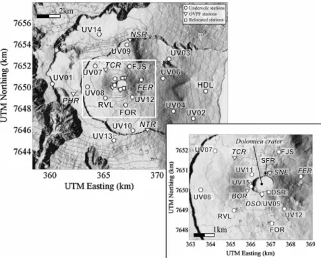
Our study focuses on rockfalls occurring in Dolomieu crater, located at the summit of Piton de la Fournaise volcano on Réunion Island. A major collapse of the Dolomieu crater floor occurred during a massive eruption of Piton de la Fournaise volcano in April 2007 [Staudacher et al., 2009]. This event considerably destabilized the crater walls and consequently increased the number of rockfalls from its edges. The dense and perma-nent seismic network set up by the Observatoire Volcanologique du Piton de la Fournaise (OVPF) on the volcano (Figure 1) has recorded numerous seismic signals generated by rockfalls, making Dolomieu crater a perfect natural laboratory to study these events.
Figure 1. Seismic network of Piton de la Fournaise volcano. The permanent stations of the Observatoire Volcanologique du Piton de la Fournaise (OVPF) are indicated by triangles and the ones installed for the UnderVolc project by circles. The names of the short-period stations are highlighted in italic. The stations indicated by squares were moved after the April 2007 Dolomieu collapse: SFR became SNE and DSR became DSO. The contour interval is 100 m.
In this paper we first present a method to automatically identify the sources of the seismic signals, focus-ing on discrimination between rockfalls and volcano-tectonic (VT) earthquakes. This method is tested on a seismicity catalog including all the 7478 rockfalls and VT earthquakes recorded by the OVPF between 1 May 2008 and 9 January 2010. A method developed to automatically pick the emergent onset and duration of the seismic signals generated by rockfalls is then presented. In the following section, the methods devel-oped to accurately locate rockfalls from the automated picking of their seismic signals are discussed, and the results are compared to rockfalls for which the location was directly observed. The automated methods are then used to determine the location of the 12,422 rockfalls listed in the OVPF seismicity catalog for the period going from 1 May 2007 to 31 April 2011. Accurate picking of the seismic signals also makes it possible to estimate the seismic energy and thus the volume of the rockfalls using the method proposed by Hibert
et al. [2011]. Finally, our methods are used to obtain maps of the locations and spatial distributions of the
number and volumes of the rockfalls that occurred between May 2007 and April 2011.
2. Automated Identification of Rockfall Generated Seismic Signals
The seismic signals of the various types of events recorded by the OVPF seismic network have specific char-acteristics that can be used to identify them manually. However, when dealing with large quantities of data, manual classification can be extremely slow and tedious and, in addition, is always subject to some degree of subjectivity. Automated classification, based on objective criteria, may be a better alternative.
Seismology allows near-real-time detection of gravitational instabilities in many different contexts. However, identification of the specific seismic signature of these events is difficult, making automation a challeng-ing task. Leprettre et al. [1998] conducted one of the first studies on this subject and proposed a method for automatically detecting snow avalanches. They used the time and frequency characteristics of the seismic signals as identification criteria. Their method was used on a data set comprising 280 events including 13 avalanches and allowed proper identification of 90% of the avalanches. In a volcanological context, auto-mated classification is more difficult as many different types of events are recorded by seismic networks.
a
db db Velocity (m/s) x 10c
Velocity (m/s) x 10 --5 -5b
Velocity (m/s) x 10 --5d
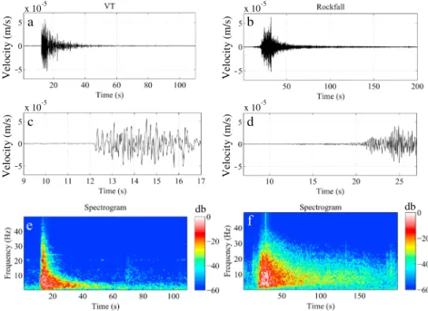
Velocity (m/s) x 10 --5Figure 2. Seismic signals of (a) a volcano-tectonic (VT) earthquake and (b) a rockfall recorded at station DSO (500 m from the crater center). Closeup of the onset of the signal generated by (c) a VT earthquake and (d) a rockfall. Spectrogram (energy given in decibels) of the seismic signal generated by (e) a VT earthquake and (f ) a rockfall.
network of the observatory of the Soufriére Hills volcano (Montserrat). That method is based on an artificial neural network and produces results that are 70% compatible with manual identifications. These authors found that a significant portion of the error came from a priori manual misidentifications. When manual misidentifications were corrected, the compatibility between automated and manual classification was 80%. We present a method designed to automatically discriminate seismic signals generated by rockfalls recorded by the OVPF seismic network (Figure 1) from those linked to volcanic or human activity. To build and test this method, a data set containing 7478 events recorded between 1 May 2008 and 9 January 2010, was used. The catalog of seismicity established by the OVPF classifies seismic events into nine different cate-gories: indeterminate, rockfall, summit volcano-tectonic (VT) earthquake, deep VT earthquake, long-period, VT earthquake outside the caldera, local earthquake, regional earthquake, T-phase (characteristic of seismic waves propagating in water), and global earthquake. Different analysts involved in the daily identification of events recorded by the OVPF seismic network based their analyses on the knowledge they had of the location of the event and on its specific characteristics in terms of waveform and frequency content. Most events have a frequency spectrum that differs from that produced by rockfalls. Therefore, a simple filtering method can distinguish rockfalls from other events. Whereas the maximum observed energy for rockfalls falls between 2 and 30 Hz, it is below 2 Hz for tectonic earthquakes (local, regional, and global). Discrimi-nating between rockfalls and VT earthquakes seismic signals is impossible by simple filtering because their frequency spectra overlap. Only 36 T-phase and 18 long-period events were identified during our obser-vation period, so we do not focus on them. The method presented here focuses exclusively on automated distinction between rockfalls and VT earthquakes. The method we propose is based on a selection of objec-tive criteria for classification of events and decision-making based on fuzzy logic techniques. The first step is to define these criteria from selected features of the seismic signals.
2.1. Features Involving Waveform and Frequency Content
Volcano-tectonic earthquakes are generated by the fracturing of rock induced by magma and gas move-ment within a volcano [Zobin, 2003; McNutt, 2005]. The associated seismic signals (Figure 2a) are char-acterized by an impulsive onset (Figure 2c) and a relatively short duration, i.e., generally less than 40 s. The spectrogram (Figure 2e) has a specific shape with a sharp energy increase followed by an exponen-tial decay of the high-frequency content with time. VT earthquakes seismic signals are characterized by a wide frequency band which can reach a maximum value of about 30 Hz and which slightly decreases with the distance between the event and the station. Seismic signals generated by rockfalls (Figure 2b)
Volcano-Tectonic Envelop Mean Max 50 100 150 -5 0 5 x 10⁻⁶ Duration (s) 50 100 150 200 200 50 100 150 Duration (s) 200 Duration (s) 50 100 150 200 Duration (s) Rockfall -12 -10 -8 -6 -4 0 500 1000 Log(A) -12 -10 -8 -6 -4 Log(A) Number 0 200 400 Number Log(Amplitude) Distribution Fitting normal law
Inc/Dec phases ti t max tf Frequency (Hz) Nro Event 0 200 400 600 800 1000 0 10 20 Frequency (Hz) Nro Event 0 200 400 600 800 1000 0 10 20 Velocity (m/s) -5 0 5 x 10⁻⁶ Velocity (m/s) -5 0 5 x 10⁻⁵ Velocity (m/s) -5 0 5 x 10⁻⁵ Velocity (m/s)
a
b
c
d
e
f
g
h
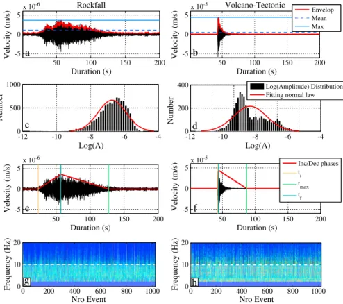
Figure 3. Seismic signal, signal envelope, signal mean, and signal maximum for (a) a rockfall and (b) a VT earthquake. Distribution of the decimal logarithm of the envelope amplitude values and the normal distribution with the same standard deviation and mean as the amplitude distribution for (c) a rockfall and (d) a VT earthquake. Increasing and decreasing phases of the signal envelope, onset time (ti), time of maximum amplitude (tmax), and final timetfof the
sig-nal for (e) a rockfall and (f ) a VT earthquake. Frequency spectrum (white for high energy, black for none) for (g) 1000 rockfalls and (h) 1000 VT earthquakes. The white dashed line indicates a frequency of 10 Hz.
are usually significantly different. They typically exhibit emergent onset (Figure 2d) and have a long dura-tion ranging from 50 to more than 200 s. In general, there is no clear maximum of the seismic signal and
Pand S waves cannot be distinguished. These characteristics are probably due to the complexity of the source mechanism and also to a dominance of surface waves in the rockfall-generated seismic signal as shown by several studies on gravitational instabilities [Deparis, 2007; Dammeier et al., 2011; N. Rousseau, Les signaux sismiques associes aux eboulements sur l’ole de La Reunion (Ocean Indien): Etude de 2 sites: La Cascade de Mahavel et la Cavite de La Soufriere, Doctoral dissertation, 1999]. The frequency band for rockfalls (Figure 2f ) ranges from 2 to 30 Hz and is centered at 5 Hz, similar to the range observed for rockfalls on the Merapi [Ratdomopurbo and Poupinet, 2000] and Montserrat [Calder et al., 2002; Luckett
et al., 2002] volcanoes. The spectrogram for rockfalls (Figure 2f ) reveals a triangular shape, similar to the
shape observed by Surinach et al. [2005], which generally reflects a linear decay of high energy in the higher frequencies.
To automate classification, we must translate the seismic-signal characteristics described above, commonly used for manual identification, into objective criteria. These criteria must be both discriminating and simple enough to ensure a short computation time. Based on characteristics identified from signal processing techniques for each type of event, five features were selected: four waveform characteristics and one frequency characteristic.
2.1.1. Ratio of the Maximum Amplitude to the Mean of the Envelope
The envelope of each signal is determined by computing the instantaneous amplitude of the seismic signal. Rockfalls usually do not have a single highly differentiable peak of maximum amplitude, whereas such a peak is always observed on the signals of VT earthquakes (Figures 3a and 3b). The ratio of the maximum amplitude to the mean of the envelope provides information on the relative strength of the maximum in comparison to the rest of the signal. This ratio should be high for VT earthquakes and low for rockfalls.
2.1.2. Kurtosis of the Envelope
Kurtosis corresponds to a measurement of the “flatness” or the “peakedness” of the distribution of a random variable with respect to a normal distribution. For a random variable X with mean𝜇 and standard deviation
𝜎, the normalized kurtosis 𝛽2of this variable is defined as
𝛽2=
E(X −𝜇)4 (E(X −𝜇)2)2 =
m4
𝜎4, (1)
where E is the expected distribution and m4the fourth central moment. The discrete form of equation (1) can be written as 𝛽2= 1 n n+1 ∑ i=1 (xi−̄x)4 ( 1 n n+1 ∑ i=1 (xi−̄x)2 )2, (2)
where n is the total number of samples, xithe value of the i-th sample, and̄x the mean over n samples.
Using equation (1), the kurtosis of a normal distribution is 3. For distributions that are flatter than the nor-mal distribution, the kurtosis values are less than 3 and the distributions are called platykurtic. On the other hand, for distributions sharper than the normal distribution, the kurtosis values are greater than 3 and the distributions are called leptokurtic.
As shown by the examples presented in Figures 3c and 3d, the distribution of the log-transformed enve-lope amplitudes is normal to very slightly leptokurtic for rockfalls. For VT earthquakes, the high amplitudes at the beginning of the signals spread out the amplitude distribution toward the higher values (Figure 3d). Hence, despite the peak centered on the lower values, the general shape of the amplitude distribution is “flatter” than the normal distribution that fits it. Thus, the amplitude distribution of VT earthquakes is rather platykurtic. The variation of the distribution for rockfalls is much less abrupt than for VT earthquakes. Skew-ness was also tested, as this statistical tool assesses the asymmetry of a distribution. Because we observed similar discrimination capabilities for kurtosis and skewness, we decided to use only kurtosis as a criterion. 2.1.3. Signal Duration
According to our observations, the duration of the seismic signals generated by rockfalls is greater than the duration of those generated by VT earthquakes. It is therefore logical to select this feature as a criterion for discrimination. Duration is given by
ΔT = tf− ti, (3)
with tithe onset time and tfthe final time when the signal returns to the noise level (Figures 3e and 3f ). 2.1.4. Duration of the Increasing and Decreasing Phases of the Signals
Rockfall seismic signals generally exhibit a slow emergence, whereas VT earthquakes are impulsive. We quantify this observation by taking the ratio of the signal rise time to the fall time as expressed by
IncDec = tmax− ti
tf− tmax, (4) where tmaxis the time at which the maximum amplitude is reached (Figures 3e and 3f ).
2.1.5. Energy in the 10–30 Hz Frequency Band
Our final criterion is based upon observations made in the spectral domain. As shown in Figures 3g and 3h, the energy at frequencies above 10 Hz is greater for VT earthquakes. We therefore compute the energy of each signal in the 10–30 Hz band computed as
Ene HF =
30Hz ∫
f =10Hz
DFT(f ) df, (5)
where DFT(f ) is the value of the power spectrum at frequency f obtained using a discrete Fourier transform of the seismic signal.
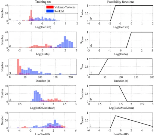
Figure 4. (a) Distribution of rockfalls (blue) and VT earthquakes (red) as a function of values of the ratio of the duration of the increasing phase to the duration of the decreasing phase of the seismic signal envelope. (b) The constructed possibil-ity function for this ratio. (c) Distribution and (d) possibilpossibil-ity function for the kurtosis value computed for the distribution of the signal envelope amplitude. (e) Distribution and (f ) possibility function for the total duration of the seismic signals. (g) Distribution and (h) possibility function for the ratio of the maximum to the mean of the signal envelope. (i) Distri-bution and (j) possibility function for the seismic energy observed in the 10–30 Hz band of the signal spectrum. When distributions overlap, the covered distribution is colored in purple.
2.2. Training Data Set
A training data set of 500 events was chosen to determine the probable range of criteria values for VT earthquakes and rockfalls. Among these events, we selected those that had clear characteristics of their respective types and for which manual identification was certain. From the initial set of 500 events, 124 rockfalls and 67 VT earthquakes were selected. The five specified criteria were computed for each of these events. The distributions of criteria values are shown in Figure 4. Except for the total duration of signals, we normalized the data using the logarithm of criteria values.
As shown in Figures 4c and 4g, criteria based on kurtosis and the ratio between the maximum and the mean of the envelope are the most discriminating, with only a small portion of their distributions overlap-ping between event types. The criteria involving the total duration (Figure 4e) and the ratio of the duration of the increasing and decreasing phases of the envelope (Figure 4a) are discriminating, but with a more substantial overlap of distributions. Finally, the criterion based on energy at high frequency (Figure 4i) is the least discriminating, with the largest overlap of the distributions. However, a certain range of values, between −2 and 0 for rockfalls and less than −2 or greater than 3 for VT earthquakes, provide a good basis for discrimination.
Thus, some parameters are very good at discriminating rockfalls from VT earthquakes and others less so. But in all cases, the distributions of these criteria for both types of events overlap. Fuzzy logic techniques provide a way to account for this uncertainty in the decision making process. These techniques offer a number of advantages: they are very simple to implement, they return information that can be easily integrated into a real-time decision process, and they require a minimum of computing resources.
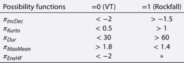
Table 1. Threshold Values Chosen for Each Criterion to Construct the Possibility Functions𝜋
Possibility functions =0 (VT) =1 (Rockfall) 𝜋IncDec < −2 > −1.5 𝜋Kurto < 0.5 > 1 𝜋Dur < 30 > 60 𝜋MaxMean > 1.8 < 1.4
𝜋EneHF < −2 ∗
2.3. Fuzzy Logic and Decision Rules Fuzzy set theory was introduced by Zadeh [1965] and makes it possible to model generally imprecise linguistic terms like “big,” “small,” or “important” to take into account the differences in behavior of a variable in a particular class. Con-sider a variable x and the linguistic term A that qualifies x. If the behavior of x is binary, for exam-ple either “small” or “large,” then A takes on the values 0 or 1 for each x qualified as “small” or “large,” respectively. However, in most cases, x does not have a binary behavior. This can result in a range of notions offered by the language, for example x can be “rather large,” etc. Fuzzy logic allows us to model A using a so-called possibility function𝜋Aof the variable x. Each
value of x is associated with a value of𝜋Aranging from 0 (false) to 1 (true). Each intermediate value of𝜋A(x)
indicates that the proposal is neither totally wrong nor totally true. If we now consider several fuzzy sets, for example, the two elementary propositions “the value of x is A” and “the value of y is B,” we can combine these sets using logical operators and assess the possibility of more complex propositions such as “the value of x is A and the value of y is B.” This statement can be translated as
Π(A, B) = 𝜋A∧𝜋B max(𝜋A∧𝜋B)
, (6)
where𝜋Aand𝜋Bare the possibility functions of fuzzy sets A and B, and ∧ is the conjunction operator.
These methods are frequently used in geosciences, for example, for data fusion for tomographic imaging [Grandjean et al., 2009; Hibert et al., 2012], characterization of seismic risk [Dong et al., 1987], or automatic detection of avalanches [Leprettre et al., 1998]. In our case, we are interested in the identification of two types of events, i.e., rockfalls and VT earthquakes. We can therefore define a hypothesis A with two options: “event n is a rockfall” or “event n is a VT earthquake.” The values of the possibility ΠA(n) related to
hypothe-sis A are chosen arbitrarily such that ΠA(n) = 1 if the event n is a rockfall and 0 if it is a VT earthquake. It is
now necessary to define possibility functions𝜋 with values ranging from 0 to 1 for each criterion, based on the a priori assumptions𝐡 on the values it would take for either a VT earthquake or a rockfall. These possi-bility functions are then integrated into the hypothesis A. Transfer functions are built from the observations as represented in Figure 4. Table 1 summarizes the threshold values chosen for each criterion, beyond which the corresponding possibility function will either take on a value of 0 or 1, depending on whether the event is a VT earthquake or a rockfall. The possibility functions𝜋 are considered linear between these two defined threshold values (Figures 4b, 4d, 4f, and 4h). The case of energy in the high-frequency band is somewhat unusual because the distribution of values for rockfalls does not stand out from those of VT earthquakes. Therefore, this function will never take on a value of 1. The maximum value is set to 0.7 at an energy value of −1. It is for this value of −1 that the rockfall distribution is most dominant. This function takes on values of 0 below −2, i.e., values below which only the population of VT earthquakes appears. The possibility function is set to decrease from 0 to 6 to reflect the increase of the domination of VT earthquakes for greater values. The possibility function𝜋EneHFis considered linear between the defined threshold values (Figure 4j).
Hypothesis A is absolutely “rockfall” when all of the possibility function values related to a priori assump-tions are equal to their respective maximums (0.7 for the𝜋EneHFpossibility function and 1 for all the others). On the other hand, hypothesis A is absolutely “VT” when all the values of the possibility functions related to a priori assumptions are equal to 0. The possibility function ΠAfor an event n can be expressed as
ΠA(n) = 𝜋IncDec(n) +𝜋kurt(n) +𝜋dur(n) +𝜋Rmaxmean(n) +𝜋EneHF(n)
5 . (7)
The function ΠAthus allows us to obtain a coefficient between 0 and 0.94 for each event. If we set a
thresh-old value at 0.5 below which the events are identified as “VT” and above which they are identified as “rockfalls,” we can obtain an estimate of the uncertainty of the identification. The greater the departure of ΠAfrom the threshold value, the more the identification is likely to be correct.
2.4. Application to Real Data
The proposed method has been tested on vertical component data recorded at station BOR (Figure 1). Signals were selected using a single criterion: a signal-to-noise ratio greater than 1.5. The data set consists
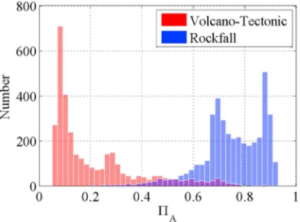
Figure 5. Distribution ofΠAvalues for the VT earthquakes (red) and rockfalls (blue) of the selected data set.
of 3343 manually classified VT earthquakes and 4135 rockfalls. Figure 5 shows the distribution of values of ΠAfor the VT earthquakes and rockfalls
of the selected data set.
Automated identification results in correct clas-sification of 88% of the events according to the classifications given by the OVPF catalog, with val-ues for the decision criterion of ΠA < 0.5 for VT
earthquakes and ΠA > 0.5 for rockfalls. In
addi-tion, 82% of rockfalls have a value of ΠAabove 0.6
and 72% of the VT earthquakes have a value of ΠAbelow 0.4. Regarding possible false identifica-tion, only 6% of rockfalls have a value of ΠAbelow
0.4 and only 8% of VT earthquakes have a value of ΠAabove 0.6. We see three main reasons for misidentification of events signals: (1) a poor signal to noise ratio (93% of the misidentified events have a signal-to-noise ratio below 3, 30% below 2, and 10% below 1.6); (2) an overlapping of two or more events with others; and (3) an a priori misidentification in the OVPF catalog. Of the 923 events misidentified by our automated method (12% of the total data set), we observe that 31% of the events manually identified as VT earthquakes are in fact rockfalls and 51% of the rockfalls are VT earthquakes. Thus, 379 events (5% of the total number of manually identified events chosen for this study) were manually misidentified. If we correct the data set of events against which we compare our automated identification method, we correctly identify 92% of the events. The identification method we have developed based on fuzzy set theory therefore seems to effectively identify rockfalls and VT earthquakes automatically from their seismic signals. These results suggest that the construction of a global identification method based on fuzzy logic is possible.
3. Automated Picking of the Onset of the Seismic Signals Generated
by the Rockfalls
In seismology, the most widely used tool for automated picking of the onset of the signal is the STA/LTA method (Short-Time-Average over Long-Time-Average) [Allen, 1982]. This method is based on the ratio of the mean of the signal amplitude computed for two sliding windows with different sizes: one short and one long. An event is detected when this ratio rises above a given threshold. The advantage of this method is that it is fast and can be used directly on raw signals. However, the necessity of subjectively defining a static threshold induces a large number of bad detections. The STA/LTA method has been improved by
Baer and Kradolfer [1987], who computed the ratio using the envelope of the signal and a dynamic
detec-tion threshold. Nevertheless, methods with thresholds prove to be ineffective for emergent signals such as those observed for rockfalls. Indeed, this kind of picker systematically picks a time after the true onset. More recent techniques are based on the Akaike Information Criterion (AIC). The AIC can detect changes in the temporal and spectral domains. This criterion may be used directly on the seismic signals [Maeda, 1985], but several studies combine this criterion with signal decomposition methods, using autoregres-sive methods [Sleeman and van Eck, 1999; Leonard and Kennett, 1999; Leonard, 2000] or methods based on wavelets [Zhang et al., 2003]. These methods are highly effective for conventional signals. However, when the signal-to-noise ratio is low and the onsets are hard to identify, as is commonly the case with rockfalls, the results are poor. Recently, new automated picking methods based on high-order statistics have been introduced [Saragiotis et al., 2002; Baillard et al., 2014]. These methods are based, for example, on the com-putation of the fourth statistical moment, kurtosis, which makes it possible to identify transitions between Gaussianity and non-Gaussianity in a signal. Such a transition coincides with the arrival of a seismic wave, making it detectable despite the presence of noise. Comparison with manual picks using several data sets showed that this method is more accurate than the commonly used STA/LTA picking tools. The ability to reduce the influence of noise led us to choose and adapt the kurtosis method for the automated picking of arrival times of the seismic signals generated by rockfalls. Another method based on the gradient of a kurto-sis characteristic function was recently used by Langet et al. [2014] for automated migration-based locating of events at Piton de la Fournaise.
0 50 100 150 200 -4 -2 0 2 4 Velocity (m/s) Time (s) 0 50 100 150 200 -4 -2 0 2 4 Time (s) 0 50 100 150 200 -4 -2 0 2 4 x 10⁻⁶ Time (s) Noise Transition Signal
-4 -2 0 2 4 x 10⁻⁷ 0 200 400 600 800 1000 Velocity (m/s) -4 -2 0 2 4 x 10⁻⁶ Velocity (m/s) Number -2 -1 0 1 2 0 100 200 300 400 500 600 700 Velocity (m/s) 0 50 100 150 200 250 300 Amplitude distribution Normal Fit
Figure 6. Distribution of the amplitudes of selected parts (identified in black) of the seismic signal and a normal distribu-tion (red curve) computed with the same mean and variance as the corresponding distribudistribu-tions. Note changes inyaxis scales on the distributions.
3.1. Automated Picking Principle
The underlying principle of our method is that noise has a normal amplitude distribution that is disturbed by the arrival of a seismic signal. It is this disturbance, and the time of the disturbance, that we want to identify.
The distribution at the transition between noise and signal has a leptokurtic behavior (Figure 6b), whereas the distributions of the signal amplitude and the noise are nearly normal (Figures 6a and 6c). A characteristic function constructed from the computation of kurtosis within a sliding window will increase in value during the transition between noise and signal (from normal𝛽2 = 3 to leptokurtic𝛽2 > 3). Thus, we can define a characteristic function CF𝛽2that will increase when a transition occurs between noise and signal for a given seismogram s(t). The characteristic function CF𝛽2of a seismic signal s(t) for a sliding window of size ΔT is defined as
CF𝛽2(t) =𝛽2(s(t − ΔT), … , s(t)). (8)
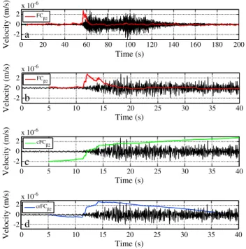
The function CF𝛽2adopts the expected behavior, exhibiting a maximum near the signal onset detectable by eye (Figures 7a and 7b). However, the maximum does not coincide exactly with the onset. Rather the onset corresponds to the time when the beginning of an increase in the values of the function CF𝛽2is observed. We must therefore identify that time. The solution proposed by Baillard et al. [2014] is to modify the function
CF𝛽2to a function that will provide a local minimum at this time. The function CF𝛽2is modified in two steps. First, the cumulative sum of the gradient of the function CF𝛽2is computed as
cCF𝛽2(k) = k ∑ i=1 𝛼i with { 𝛼i= F𝛽2,i+1− F𝛽2,i if (CF𝛽2,i+1− CF𝛽2,i)≥ 0 𝛼i= 0 otherwise . (9)
Thus, the inflection point of the function cCF𝛽2indicates the time of the onset (Figure 7c). For that point to become a local minimum, a linear correction must be applied to the function cCF𝛽2. The slope between the minimum and maximum of the function cCF𝛽2is computed, and each point is adjusted so that the maximum and minimum of the new resulting function crCF𝛽2become 0:
crCF𝛽2(k) = cCF𝛽2(k) − (k − 1) ×cCF𝛽2
(n) − cCF𝛽
2(1)
n − 1 − cCF𝛽2(1), (10)
where n is the number of points in the window. The time corresponding to the minimum of the function
0 20 40 60 80 100 120 140 160 180 200 -2 0 2 x 10⁻⁶ Time (s) Velocity (m/s) -2 0 2 x 10⁻⁶ Velocity (m/s) FC 0 5 10 15 20 25 30 35 40 Time (s) -2 0 2 x 10⁻⁶ Velocity (m/s) 0 5 10 15 20 25 30 35 40 Time (s) -2 0 2 x 10⁻⁶ Velocity (m/s) 0 5 10 15 20 25 30 35 40 Time (s) FC cFC crFC
a
b
c
d
Figure 7. (a) Seismic signal of a rockfall and corresponding charac-teristic functionCF𝛽2. (b) Closeup of the onset of the seismic signal and corresponding characteristic functionCF𝛽2. (c) Seismic signal and corresponding cumulative characteristic functioncCF𝛽2. (d) Seismic signal and corresponding “de-trended” cumulative characteristic functioncrCF𝛽2.
The arrival time picked by this character-istic function depends on the frequency content f of the seismic signal and the length ΔT of the sliding window chosen. A small window will be more sensi-tive to small-scale variations, whereas larger windows will depend mostly on large-scale variations. To mitigate the errors caused by this dependence, the characteristic functions are computed simultaneously for multiple frequency bands and different sizes of sliding win-dows. The mean𝜇 of all these functions is then computed and provides a single characteristic function that integrates all the information. Thus, the onset time tiis
given by
ti= min(𝜇(crCF𝛽2(ΔT, f))) (11) 3.2. Protocol
To apply our automated picking method, we must define three inputs: (1) the sig-nal (in whole or part), (2) the window sizes, and (3) the frequency bands to be used. After numerous tests, the following protocol was chosen. A STA/LTA detector is first applied to a seismic signal, previously identified as an event, in order to roughly estimate the arrival time of the signal. The function crCF𝛽2is then computed on a portion of the signal beginning 20 s before the arrival time picked by the STA/LTA and continuing until the time corresponding to the maximum of the signal envelope. If this time is less than 10 s, it is set to 10 s. This gives us a preliminary arrival time. Then, the function crCF𝛽2is computed on 20 s of signal, centered on the preliminary arrival time, i.e., 10 s before and 10 s after. For these two successive steps, the same parameters of window size and frequency band are chosen: window sizes of 2, 3, 5, and 10 s and four respective frequency bands of 2–7 Hz, 5–10 Hz, 7–12 Hz, and 10–15 Hz. Lastly, the end of the signal must be identified. Once the event onset has been identified, we determine the level of preevent noise by computing the mean of a smoothed envelope (moving average over 200 samples equivalent to 2 s). This mean gives a threshold value Sfwhich, when reached by the signal
envelope after the identified arrival of the signal, gives the final time tfof the rockfall seismic signal. In
prac-tice tfis determined when the smoothed signal envelope drops below 1.1 × Sf. An example of the results
obtained by the application of this protocol to a rockfall-generated seismic signal is shown in Figure 8. From the picked first arrival, we can estimate the signal-to-noise ratio (SNR). In our study, we define SNR as the ratio of the median of the signal envelope over the 20 s immediately following the picking to the median
𝜇1∕2of the envelope of the noise observed during the 10 s before the picking. Here we prefer to use the median because, unlike the arithmetic mean, it is not unduly influenced by a few outliers.
SNR =𝜇1∕2(uenv(ti, … , ti+ 20)) 𝜇1∕2(uenv(ti− 10, … , ti))
(12) 3.3. Comparison of Automated and Manual Picking: Error Estimate
To estimate the accuracy of our time-picking method, we compared automated and manually picked arrivals of 759 rockfalls recorded by vertical-component data at stations BOR, DSR, SFR, TCR, FER, NSR, NTR, and PHR (Figure 1). The distribution of the time differences𝜖pbetween manual and automatic picks show
that 31% of the picks have a difference of less than 0.1 s, 64% a difference less than 0.5 s and 79% a differ-ence less than 1 s (Figure 9). These results are fairly good considering the difficulty of manually picking the onset of seismic signals that are as emergent as those generated by rockfalls.
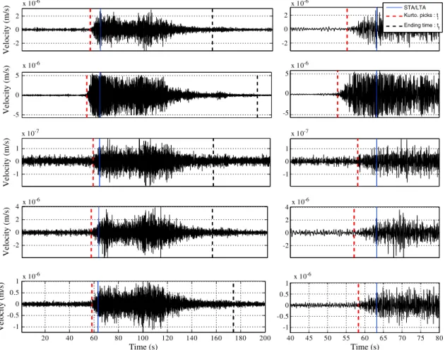
-2 0 2 Velocity (m/s) Velocity (m/s) Velocity (m/s) Velocity (m/s) Velocity (m/s) -5 0 5 x 10-6 x 10-6 x 10⁻⁶ -5 0 5 x 10-6 x 10-7 -2 0 2 -1 0 1 x 10⁻⁷ -1 0 1 -2 0 2 4 x 10 -6 -2 0 2 4 20 40 60 80 100 120 140 160 180 200 -1 -0.5 0 0.5 1 x 10 -6 -1 -0.5 0 0.5 1 Time (s) 40 45 50 55 60 65 70 75 80 Time (s) STA/LTA Kurto. picks : t i Ending time : t f
Figure 8. Example of event onset and duration picking given by the STA/LTA (blue line) and kurtosis (dashed red line) of a seismic signal recorded at five stations: BOR, DSO, SFR, FER, and TCR (Figure 1). Panels to the right show detailed views of the onset of each signal.
The quality of the picked onset depends on the SNR: the onset of a strong signal is easier to identify both manually and by our method (Figure 10). The relationship between pick quality and SNR can be used to obtain a rough estimate of the inherent uncertainties when applying our automated picking method to a large data set. The relationship between SNR and picking error (in seconds) can be approximated by the following regression function:
𝜖p= 0.06 + 1.2 exp−0.4905 SNR (13)
Figure 9. Histogram of the distribution of the difference𝜖p(s) between automated and manual picking of the onset of the rockfall seismic signals.
Despite the difficulties caused by the emergent nature of rockfall seismic signals, the method we propose proves to be efficient and accurate for picking onsets of rockfall signals. This accu-racy allows us to establish methods for locating the rockfalls based on the onset times of their signals.
4. Locating Rockfalls on Piton de la
Fournaise Volcano
Event location is important information when trying to assess hazards linked to rockfalls. In addition, the spatiotemporal activity of rockfalls within Dolomieu crater may carry information on the deformation of the summit
Figure 10. Median value of the difference of𝜖p(s) between automated and manual picking of the onset of the rockfall seis-mic signals, depending on the signal-to-noise ratio (SNR), and curve (red) of the regression function that best fits the data.
of Piton de la Fournaise volcano. However, the characteristics of seismic signals generated by rockfalls, i.e., slow emergence, generally low signal-to-noise ratio, and lack of a single highly differentiable maximum amplitude and clearly recognizable phases, make methods usually used in seismology difficult to apply. Another difficulty is that rockfalls generate relatively weak seismic signals that are recorded by only a small number of stations. We must therefore overcome these difficulties to establish loca-tion methods that are accurate, robust, not very demanding in terms of signal quality (low SNR and few phases) and quantity, and inexpensive in terms of computation time, because of the large amount of data to be processed. Few methods aimed specifically at locating rockfalls have been developed. Among those that exist, it is possible to distinguish two approaches: one based on signal arrival time and an other on the energy or amplitude of the signal. Among the studies using the first approach, Helmstetter and Garambois [2010] proposed a method based on cross correlation of signals recorded at different stations to measure the difference between the arrivals and then a grid search for the point that maximizes the cross-correlation traces. This method is suitable when there is a dense network of seismometers arranged as antennas at distances very close to the initiation zones of rockfalls (less than 100 m), which is not the case at Piton de la Fournaise. Another method, using the second approach and proposed by Battaglia and Aki [2003], is based on a model of attenuation of the amplitude of the seismic signal generated by rockfalls. A grid search is conducted to seek the minimum of the differ-ence between modeled and observed amplitudes, thus providing an estimate of the location of the rockfall. This method requires high accuracy for the observed amplitudes, which must be corrected for site effects at each station. However at Piton de la Fournaise, there were significant changes in the seismic network over the period of interest. In particular, two stations (SFR and DSR) were moved away from the Dolomieu crater edges for safety reasons. The uncertainty regarding site factors and the parameters that control the exact computation of amplitudes made the tests we conducted using this method inconclusive. As a result, we decided to use the automated picking of arrival times because only a few parameters influence the observable data and because an automated picking method allows us to quantify the picking and hence the location errors.
Our approach to locating rockfalls involves two main assumptions. (1) The shallow part of the volcano, constituted by many eruptive deposits, is very heterogeneous but insufficiently characterized to have a rea-sonable 3D (or 2D) velocity model. Therefore, we assumed a constant average velocity and tested many dif-ferent values for this velocity. (2) The seismic signals generated by rockfalls at Piton de la Fournaise volcano are dominated by Rayleigh waves, as observed in other contexts by Deparis et al. [2007] and Dammeier et al. [2011]. Therefore, we need to predict travel times of high-frequency waves propagating along the surface. In the case of Piton de la Fournaise volcano, the prediction method must account for highly varied topog-raphy. The location methods that we describe in this section are based on a grid search, implying that observed and predicted travel times between all grid locations and all stations must be systematically com-pared for many thousands of events. In this case, the best strategy is not to compute these travel times on the fly but to use precomputed tables. These tables must be computed on a 2-D grid (X, Y) and the com-putation must account for the difference in elevation (and possibly in local seismic velocities) between the grid points. For this, a strategy involving three successive steps has been designed. (1) Compute a map for each station which gives the topographical distance between it and all other points of the grid of the digi-tal elevation model used. (2) Transform the distance maps into travel time maps by dividing by a constant velocity. (3) Search for the best location by minimizing the discrepancy between arrival times picked by the automated method and modeled travel times extracted from the travel time maps. The method used to
Figure 11. Map of the RMS values computed with the RMS locating method for a rockfall that occurred on 8 August 2008 with an optimal velocity model of 720 m/s. The minimum RMS value is indicated by a black diamond. The contour of the Dolomieu crater is indicated by the black dotted line.
construct the distance maps is dis-cussed in Appendix A. The methods used to determine the best loca-tion from the travel time maps are detailed in the following sections. 4.1. Location Methods
The two methods that we propose use the arrival times tn
obs, picked with the kurstosis-based algorithm described above. The first method, that we have called “RMS,” like the amplitude-based method by
Battaglia and Aki [2003], computes
the root mean square (RMS) dif-ference between theoretical and observed arrival times for each point of a grid. The second method, that we have called “hyperbola,” is related to the “maximum intersection method” by Font et al. [2004] and is also known as the “station-pair double-difference method” [Zhang et al., 2010; Haney, 2010]. Its simplicity greatly reduces the computation time compared to the RMS method while maintaining satisfactory accuracy and error handling characteristics.
The first approach we propose to determine the best location is to test each point (i, j) of a grid as a potential source. We consider distance maps that give the distance rn
ijalong the topography between the point (i, j)
and the station n. The speed of propagation of the wavefront is also a search criterion. For each point, k velocity models Vkare tested, where Vk= V0+ k ∗ dV. V0is the lowest speed tested and dV is the constant interval between two successive velocities tested. Assuming a homogeneous, isotropic medium in which seismic waves propagate at a constant speed Vk, following the topography, the theoretical time it would take for the wave at a point (i, j) to reach station n is simply
tn comp= rn ij Vk , (14) where rn
ijis the topographical distance between the source point (i, j) and the station n. The discrepancy
between the computed time tn
compand the picked time tnobsis given by equation
RMS(xi, yj, Vk) = √ √ √ √ 1 N N ∑ n=1 (tnobs− tn comp)2 (15)
The coordinates (xmin, ymin) at which equation (15) is minimized for a speed Vminindicate the location of the source. The RMSminvalue quantifies the error in the location of the event. However, despite the use of precomputed time maps, this method is time consuming. The optimal location (Figure 11), on a 1300 × 1300 point grid with a 10 m resolution was obtained for a velocity of 720 m/s after testing six different velocity models Vk(240, 360, 540, 660, 720, and 800 m/s). It gives a minimum RMS value of 0.49 s. The RMS value is
influenced by improper arrival time picks at one or more stations. We therefore propose a second method based on the differences of travel times and the stacking of the resulting hyperbolas. This method will not cover our entire grid but allows us to eliminate outlying picks.
Let tn
obsbe the time picked at station n and T
n
ij the whole time map for the same station, giving t n
compat any point (i, j) of the grid, for a speed Vk. The time map Tijncan be computed as
Tn ij =
rn ij
a
b
c
Figure 12. (a) Time map (in seconds)TijBORcomputed for BOR sta-tion. (b) Delay map (in seconds)ΔTijBOR,DSRcomputed for the pair of stations BOR-DSR. (c) HyperbolaHBOR,DSRij showing possible source locations for the pair of stations BOR-DSR.
These time maps are computed for the N stations of the seismic network we want to use (Figure 12a). Let Δtn,m = tobsn − tmcomp be the difference of the observed tn
obsand computed tcompmarrival times at stations
nand m, respectively. We can define a delay map ΔTijn,m(Figure 12b), computed between each pair of stations n, m for each grid point (i, j) from time maps defined by equation (16):
ΔTijn,m= Tijn− Tijm (17) By finding the value Δtn,mon the ΔTijn,m map for the pair of stations n, m, a hyper-bola will be defined (Figure 12c). In practice, a new map Hn,mij is built with a value of 1 when the value of ΔTijn,mis equal to Δtn,m±𝛿t and 0 elsewhere: Hn,mij = { 1if Δtn,mobs−𝛿t < ΔTijn,m< Δtn,mobs+𝛿t 0otherwise (18) where𝛿t is a time interval dependent on the accuracy of the picking of the arrival time. Each hyperbola will indicate a potential location area of the source. By computing Hn,mij maps for each pair of stations n, m and then stacking all the maps obtained, the hyperbolas will focus at a point that minimizes the difference Δtobsn,m− ΔTi,jn,mfor each pair of stations
n, m. Finally, we can estimate the error
in the same way as for the RMS method, but this time by computing the theoreti-cal time from the point (imax, jmax) where
Nphyperbolas focus. Subscript p indicates
from which pair of stations the focusing hyperbolas have been computed:
RMS(xi, yj, Vk) = √ √ √ √ √ 1 Np Np ∑ p=1 (tpobs− tpi max,jmax) 2, (19) where Vkis the velocity of the chosen model. The whole process is repeated using the velocities within the interval defined above. The minimum value of the RMS function is sought among all the velocity models that give the maximum number of focusing hyperbolas (Figure 13). This “hyperbola” approach has two major advantages over the RMS method: (1) the computation of maps is very fast because we only make simple operations on existing grids that are reusable for different events and (2) it allows us to exclude aber-rant observed arrival times by not using hyperbolas corresponding to the stations where the picking is bad. In extreme cases, when the travel times are inconsistent, no point meets the requirements for the Hn,mij map to take on a value of 1. Finally, the choice of the parameter𝛿t in equation (18) accounts for uncertainties introduced by the picking method. Equation (13) gives an estimate of the picking error𝜖tas a function
Figure 13. Stacking of all the computed hyperbolas using the “hyperbola” method for locating a rockfall that occurred on 8 August 2008, using an optimal velocity model of 720 m/s. The color bar indicates the number of overlapping hyperbolas. The contour of the Dolomieu crater is indicated by the white dotted line.
of signal-to-noise ratio. Let𝜖tnand𝜖tmbe the
picking errors in the signals recorded for two stations n, m. The parameter 𝛿tn,mfor this pair of stations is defined as the arithmetic mean of these errors𝛿tn,m= (𝜖tn+𝜖tm)∕2.
The focusing of the hyperbolas giving the loca-tion of a rockfall that occurred on 8 August 2008 is shown in Figure 13. This results was obtained with six speeds Vktested (240, 360, 540, 660, 720, and 800 m/s) and a 1300 × 1300 point grid with a resolution of 10 m. The optimum value of the speed is 720 m/s and the RMS value is 0.087 s. For this specific event, the “hyperbola” method reduced the error compared to the RMS method while offering a more coherent location, i.e., at the edge of the Dolomieu crater. With our com-puting capability, using the “hyperbola” method reduces the computing time by a factor of 300 compared to the RMS method.
4.2. Location Errors
When locating events, it is important to assess the spatial accuracy of the methods used. Therefore, a rela-tionship has to be found between errors of the methods in the form of RMS time residuals and the true spatial error in meters. We arbitrarily define a synthetic point source in the center of the Dolomieu crater. All other grid points are tested as potential sources. An RMS map comparing the time computed using the model for the exact position of the source and the time computed for all other grid points is created.
RMS (s)
RMS (s)
a
b
Figure 14. (a) Mean, maximum, and minimum rockfall spatial errors in locating rockfalls as a function of the RMS value for a velocity model of Vk= 600m/s. (b) Rockfall location errors as a function of the RMS value for six different velocity modelsVk.
The RMS map is then compared to the distance map between each point of the grid and the synthetic source. Maximum, mean, and minimum dis-tances from the source as a function of the RMS values are shown in Figure 14. The relationship between the mean spa-tial error and the RMS value is almost linear. The least-squares regression line fitting the mean spatial errors gives us the following equation linking the spa-tial error𝜖dand the RMS time residual, for
any speed Vk:
𝜖d= 1.56Vk× RMS (20)
Finally, we must integrate into the location error the signal onset picking uncertainty, given by equation (13). An estimate of the total spatial error Edon the position of each event is therefore given by
Ed=𝜖d+ Vk𝜇(𝜖p) (21) 4.3. Validation on Known Events We tested our methods using two known rockfalls that occurred on 23 and 24 September 2011. They were recorded by
V
elocity (mm/s)
Time (s)
Figure 15. (a) Seismic signals generated by the 23 September 2011 rockfall recorded by stations BOR, DSO, and SNE. (b) The best location provided by the “hyperbola” method, obtained with a velocity model of 360 m/s. (c) The best loca-tion provided by the RMS method, obtained with a velocity model of 360 m/s. (d) Localoca-tions of rockfall determined from each method. The magenta diamond indicates the RMS best location and the blue diamond indicates the “hyperbola” best location. In this case, the two locations overlap. The orange diamond indicates the actual location of the rockfall estimated from videos. The red circle has a radius of 70 m, equal to the spatial location error in given by equation (21).
seismically triggered cameras. Other rockfalls were observed by the cameras, but only these two generated seismic signals were detected by at least three stations. We used a 1300 × 1300 point grid that covered the entire Piton de la Fournaise area with a spatial resolution of 10 m. Nine different velocities models Vkwere
tested (k = 1, 2, … , 9), with V0= 360 and dV = 120 m/s, giving the following velocities: 360, 480, 600, 720, 840, 960, 1080, 1200, and 1320 m/s. This range of velocities is realistic for surface waves propagating in the shallow layers of Piton de la Fournaise volcano.
The locations obtained for the 23 September 2011 rockfall are identical regardless of the method used and are very close to the observed source area (Figure 15). The RMS value obtained by both methods is 0.092 s, which is very low. The computed spatial error confirms the quality of the location as the circles representing the spatial error cover the actual location. Note however that this excellent location was obtained using a very low seismic velocity model of 360 m/s. The locations obtained for the 24 September 2011 rockfall differ slightly depending on the method used (Figure 16). The position given by the RMS method is slightly closer to the actual location. However, taking into account the spatial error for both methods gives circles that include the actual position. The optimal location for this event is obtained for a seismic velocity model of 720 m/s for both methods. The seismic velocity values obtained for the two rockfalls are different even though these events are very close spatially. This observation is discussed further in the next section. Despite the strong assumptions and simple propagation model used, the hyperbola approach seems to be efficient and accurate. The computation of spatial errors in equation (21) gives accurate estimates of locations. In addition, good results are obtained even when only three stations are used. The “hyperbola”
Figure 16. (a) Seismic signals generated by the 23 September 2011 rockfall recorded by stations BOR, DSO, and SNE. (b) The best location provided by the “hyperbola” method, obtained with a velocity model of 720 m/s. (c) The best location provided by the RMS method obtained with a velocity model of 720 m/s. (d) Locations of rockfalls determined from each method. The magenta diamond indicates the RMS best location and the blue diamond indicates the “hyperbola” best location. The orange diamond indicates the actual location of the rockfall estimated from videos. The red circle has a radius of 130 m, equal to the spatial location error in given by equation (21).
method fulfills all the necessary criteria to enable us to precisely study the spatial evolution of the rockfall activity occurring in Dolomieu crater.
5. Application to the Rockfalls Occurring Within Dolomieu Crater From May 2007
to May 2011
The methods we have developed make it possible to handle large amounts of data to determine the loca-tions of hundreds of rockfalls. We focus our study on the period ranging from the collapse of the Dolomieu crater in May 2007 to the dismantling of the stations installed for the UnderVolc project in April 2011 [Brenguier et al., 2012]. The dates and times of all events that occurred during this period were extracted from the catalog of seismicity provided by the OVPF. According to the OVPF catalog, 12,422 rockfalls were identified during this period. Of these, 4270 could not be picked by our automated method at more than two stations: either not enough stations recorded these events or the automated picking method was not able to find consistent arrival times for them. The excluded rockfalls are likely to be the smaller ones that did not generate a seismic signal strong enough to be recorded on more than two stations or to emerge from the background seismic noise.
5.1. Discussion on Locations
Rockfalls were located using the “hyperbola” method. To determine the best seismic velocity model, six were initially tested. Values for the constant seismic velocity of these models were chosen from a range of potentially realistic values for surface waves propagating in the shallow layers of Piton de la Fournaise
Table 2. Values of the ParametersaUsed to Test the Best Velocity
ModelVfor Locating Rockfalls With the “Hyperbola” Method V(m∕s) Number 𝜇(RMS) 𝜇(𝜇1∕2(Δt)) 𝜇(𝜎(Δt)) 400 4356 1.56 −0.312 4.43 600 4144 1.43 −0.038 3.88 800 3865 1.36 0.014 3.63 1000 3655 1.42 0.016 3.72 1200 3446 1.39 0.011 3.70 1400 3213 1.42 0.008 3.70
aNumber of events located, average RMS value𝜇(RMS)provided
by the “hyperbola” method, and mean over all the stations of the median𝜇1∕2(Δt)of the standard deviation𝜎(Δt)of the difference between the computed arrival timestn
compand the observed arrival
timestnobspointed for stationn. Optimum values for each parameter are indicated in bold.
volcano: 400, 600, 800, 1000, 1200, and 1400 m/s. For each of these models, the number of events located, the aver-age RMS value𝜇(RMS) provided by the method, and the average, over all the stations, of the median𝜇1∕2(Δt) of the standard deviation𝜎(Δt) of the dif-ference Δt between the computed time
tn
compand observed time t
n
obsfor a station
nwere computed. Table 2 gives the val-ues of these parameters for each velocity model tested.
No optimal velocity model emerges. The maximum number of events was located using the slowest model. However, it is for this model that the highest values of the average RMS and of the mean of the median difference Δt are observed. This indicates that even though this model allows us to locate more events, it is also the one that introduces the largest errors. The best compromise between location quantity and quality is obtained for the 800 m/s velocity model. We therefore located these events a second time using a refined velocity range that varied up to 20% from the optimal velocity (800 m/s). We chose a value of 20% variation because
Brenguier et al. [2007] showed that Rayleigh-wave velocities varied up to 15% at depth. We increase this
vari-ation by 5% because we expect surface layers to be even more heterogeneous. The locating algorithm is applied as described in section 3.2, testing nine different speeds, with values of 640, 680, 720, 760, 800, 840, 880, 920, and 960 m/s. Of the 8152 events which signal onset was successfully picked on three stations or more, 3655 rockfalls could not be located because the hyperbolas were not focused. Thus, 56% of rockfalls recorded on more than two stations were located.
The majority of the events (about 62%) were located with an RMS value less than 1 s (Figure 17a). In addi-tion, 59% of the events have an RMS value less than 0.5 s and 45% an RMS value less than 0.1 s, which corresponds to 2014 events located with an accuracy of about 100 m. As shown in Figure 17b, the major-ity of the events were located using only three or four stations. The average ratio between the number of stations on which a picking was obtained and the number of stations used to obtain the optimal loca-tion is 0.7. Figure 17c shows the distribuloca-tion of the tested velocity values. This distribuloca-tion shows that the extreme values (640 and 960 m/s) of the velocities tested provided the best solutions. The fact that we use a topography-adjusted, homogeneous velocity model, whereas the near-surface of Piton de la Fournaise volcano is highly weathered and fractured, and hence seismic velocity highly heterogeneous within this medium, may explain this observation.
To illustrate this point, we use frequency-time analysis [Levshin et al., 1989] to measure group velocities of surface waves extracted from noise cross correlations between pairs of stations. The velocities are highly variable, with a minimum value of 400 m/s for the SNE-UV05 path (Figure 18a) and a maximum of 1000 m/s for the SNE-UV15 path (Figure 18b), for a frequency of 3Hz. These values are similar to optimal veloc-ity models presented in Table 2, used in rockfall locating. Furthermore, the Rayleigh waves propagating in the shallow parts (at a maximum depth of about 100 m) of the volcanic edifice are highly dispersive and their velocities vary greatly, depending on the frequency of the signal. The higher the frequency, the slower the velocities. When looking at the frequency content of the two directly observed rockfalls (Figure 19), we observe that the frequency spectrum of the second rockfall exhibits more energy in the lower frequencies, with a peak at 1 Hz, whereas the first rockfall exhibits a peak around 5 Hz. This simple comparison shows how the dominant frequency of the rockfall seismic source combined with the dispersive nature of the Rayleigh waves affects the propagation velocity of the rockfall-generated seismic waves. This analysis high-lights the strong need for a more complex velocity model. Moreover, taking into account the frequency content of the seismic signal generated by rockfalls might also increase substantially the accuracy of the locating methods.
Figure 17. (a) Distribution of the RMS values provided by the “hyper-bola” locating method applied to our data set of 12,422 rockfalls. (b) Distribution of the number of stations used to locate rockfalls for the period studied. (c) Distribution of the velocity models giving the optimal locations.
5.2. Volume Estimation
The computation of rockfall volumes is based on the work presented in Hibert et
al. [2011], who found that for the
rock-falls occurring within Dolomieu crater, the seismic and the potential energies of a rockfall were linked. The volume
Vof an individual rockfall can be estimated using
V = 3Es
Rs∕p.𝜌cgL(tan𝛿 cos 𝜃 − sin 𝜃)
(22) The density𝜌c = co𝜌i, where𝜌iis the
density of intact rock (2000 kg m−3) and cois the volume fraction of the solid material (0.6). A value of L = 500 m was chosen for the approximate slope length. A value of the mean angle of the slope𝜃 = 35◦was chosen from the friction coefficient estimated through simulations presented by Hibert et al. [2011], calibrated to give realistic mod-eled rockfalls duration.𝛿 is the mean angle between the deposit and the slope. As the deposit is almost par-allel to the slope,𝛿 is quasi-null, i.e.,
𝛿 = 0. Rs∕pis the average ratio between
the seismic and potential energies. A value of Rs∕p= 5 × 10⁻⁴was used for this
parameter. A first approximation of the seismic energy Es, assuming an isotropic
homogeneous propagation medium, a point-force source and seismic signals dominated by surface waves, is given by
Es = t2 ∫ t1 2𝜋r𝜌hc uenv(t)2e𝛼rdt (23) where uenv(t) = √ u(t)2+ Ht(u(t))2, (24)
Figure 18. Period-velocity diagrams, showing the energy of the seismic noise normalized by period band, used to iden-tify the group velocity dispersion of Rayleigh waves, computed between (a) stations SNE and UV05 and (b) stations SNE and UV15, located on the edge of Dolomieu crater. The dashed line represents the dispersion curve of the dominant energy level of the Rayleigh waves. (c) Locations of the stations used.
Figure 19. Normalized Fast Fourier Transform (FFT) of the seismic signals recorded at DSO station and generated by (a) the 23 September 2011 and (b) 24 September 2011, rockfalls.
where t1and t2are, respectively, the picked onset and final times of the seismic signal, r is the distance between the event and the recording station, h the thickness of the layer through which surface waves propagate,𝜌 the density of the ground, and c the group velocity of the seismic waves [Crampin, 1965;
Vilajosana et al., 2008]. uenv(t) is the amplitude envelope of the seismic signal (here the ground velocity) obtained using the Hilbert transform (Ht) and𝛼 is a damping factor that accounts for inelastic attenuation of the waves [Aki and Richards, 1980]. This damping factor is frequency dependent and is computed as
𝛼 = f𝜋
Qc (25)
We impose a frequency f = 5 Hz, because this is the center of the frequency band where most of the energy is observed for granular flows. On the basis of the typical group velocity for surface waves in volcanic areas and the optimal velocity given by our locating method, we assume a group velocity of c = 800 m/s and a quality factor accounting for the attenuation of seismic wave Q = 50, which is within the range of values obtained by Koyanagi et al. [1992] for Kilauea volcano. We assume a rock density of𝜌 = 2000 kg m−3, a common value for volcanic rock. For each event successfully picked by the automated method, the average seismic energy was computed on the stations closest to the crater for the period studied: BOR, DSO(R), SNE, UV05, and UV11. These stations were chosen because all the events were recorded on at least one of them, which ensures consistency in the computation of the volume for the entire period. The cumulative volume of all rockfalls that occurred during the period studied was estimated at 3.23 Mm3, with individual volumes ranging from 1 m3to 60 × 103m3.
5.3. Spatial Evolution of Rockfall Activity
We can now trace the location and spatial distribution of rockfalls for a period ranging from 1 May 2007, just after the Dolomieu crater floor collapse, to 1 April 2011. Most of the rockfalls are located on the Dolomieu crater slopes (Figure 20a). The spatial distribution maps of the number and volumes of rockfalls (Figures 20b and 20c) were constructed by assigning the corresponding values to circles centered on their locations. The radii of these circles have a constant value equal to the median of the spatial rockfall locating error. The median of the RMS values for these events is 0.14 s, and thus, the corresponding spatial error given by equation (20) is approximately 180 m (equation (20)). This choice was made to prevent rockfalls with high spatial errors and large volumes from dominating this representation and to provide better visibility of all the events. The final maps are obtained by stacking all the circles corresponding to the rockfalls that occurred during the selected period.
Throughout the four years studied, the rockfall activity appears to be most intense in the western part of Dolomieu crater, at its junction with Bory crater. There, more than 700 rockfalls had a cumulative mobilized volume of approximately 3.5 × 10⁵m3(Figures 20b and 20c). The Bory-Dolomieu junction was strongly affected by the crater floor collapse [Michon et al., 2007; Staudacher et al., 2009]. In the months following this catastrophic event, destruction of large parts of the cliff overlooking Dolomieu crater was witnessed [Hibert
et al., 2011]. This made the area extremely unstable and thus prone to numerous and large rockfalls. Two less
active areas are located in the south eastern and northern parts of Dolomieu crater, close to the remains of Soufrière cavity that was destroyed by the Dolomieu crater collapse.