HAL Id: hal-01701827
https://hal.archives-ouvertes.fr/hal-01701827
Submitted on 6 Feb 2018
HAL is a multi-disciplinary open access
archive for the deposit and dissemination of
sci-entific research documents, whether they are
pub-lished or not. The documents may come from
teaching and research institutions in France or
abroad, or from public or private research centers.
L’archive ouverte pluridisciplinaire HAL, est
destinée au dépôt et à la diffusion de documents
scientifiques de niveau recherche, publiés ou non,
émanant des établissements d’enseignement et de
recherche français ou étrangers, des laboratoires
publics ou privés.
Solving the Flight Radius Problem
Assia Kamal Idrissi, Arnaud Malapert, Rémi Jolin
To cite this version:
Assia Kamal Idrissi, Arnaud Malapert, Rémi Jolin. Solving the Flight Radius Problem. 7th
Interna-tional Conference on Operations Research and Enterprise Systems (ICORES 2018), Jan 2018, Funchal,
Portugal. pp.304-311, �10.5220/0006654003040311�. �hal-01701827�
Solving the Flight Radius Problem
Assia Kamal Idrissi
1, Arnaud Malapert
2and R´
emi Jolin
11
Milanamos, 1047 route des Dolines, Sophia Antipolis, France
2
Universit´e Cˆote d’Azur, CNRS, I3S, France
{assia.elafouani, remi.jolin}@milanamos.com, [email protected]
Keywords:
Flight Radius Problem, Airline Schedule Design, Shortest Path Algorithms, Regret.
Abstract:
In this article, we present the flight radius problem on the condensed network. This problem consists of locating in the network what routes represent business opportunities that are attractive regarding time or cost criteria, and passing through a specific flight. We introduce a regret function to model the regret compared to the optimal value of such criteria. We work with a startup company specialized in air transportation. The company has developed a decision tool for airline managers to analyze and simulate a new market. Our problem is derived from this application. Thus, we start by formulating the problem as finding a maximal sub-graph such as for each node, there exists a valid path by the regret function. Then, we propose two methods for solving the problem. One using procedures of the graph database Neo4j where the condensed network is stored. The second one is a new algorithm based on Dijkstra algorithm. Finally, we have been able to report results on a set of real-world instances, based on different (OD) pairs and various values of the regret, studying the impact of considering different combinaison of node’s type: Hub & Spoke.
1
INTRODUCTION
The air transportation industry has evolved rapidly over the last years. The growth of air pas-senger demands has pushed airlines to enhance their quality of service. The airlines should focus on the route network development which is con-sidered as the initial problem addressed by the airlines. It aims to determine a set of routes to be operated in an airline’s network. It takes pas-sengers demand, airport, aircraft characteristics, and then generate a set of origin-destination pairs (OD) to serve, the schedule design problem aims to define the frequency and departure time of each flight.
Airlines have the choice to create a new route to serve a new destination, this new route pro-vides connecting traffic to other flights, or to in-crease/decrease the frequency of existing routes. The first requires the route network development problem and the schedule design problem which demand a lot of investment. While in the sec-ond, the airline network already exists. The prob-lem of allocating a new flight is related to these
problems. The problem consists of determining a set of (OD) pairs to serve and then choose flight schedules with respect to the quality of service index (QSI) model. QSI is a market share model used by most of airlines to estimate their part of the market (Jacobs et al., 2012). We define a flight by three attributes: Origin-Destination (OD) pair (an OD pair is a couple of airports), arrival/departure time and aircraft type. We dis-tinguish between three different types of flights: A non-stop flight is a single flight with no inter-mediate stops. In the absence of such flights, pas-sengers must take either a direct flight or a con-necting flight. A direct flight is operated by the same aircraft and includes at least one stop. A connecting flight is a flight where passengers have to change of the aircraft in a hub. A route is a sequence of flights with unique flight numbers that begins at the origin airport and ends at the destination airport (Hall, 2012).
The problem of allocating a new flight evokes design and visualization of the airline’s network. However, the network is so large that it cannot be visualized. Thus, we proposed the flight
ra-dius problem which is related to the route net-work development problem. This problem con-sists in showing only interesting airports with re-spect to a specific flight regarding the QSI crite-ria. Cost and time are the major QSI criteria of this model. Besides, the regret criterion is com-pared to the optimal time or optimal cost. The main idea of the flight radius problem is to locate in the network what routes, passing through a specific flight, and represent business opportuni-ties that are attractive to the passengers accord-ing to different preferences. The choice depends on the passengers since they have different prefer-ences over the criteria, and type of flight is one of these criteria. For this reason, these preferences should be taken into consideration in this prob-lem; it is modeled by the regret function. The function aims to model the regret compared to the optimal value of cost or time. The visual-ization is a simple way to remove the irrelevant routes. Since the airline network exists already, our aim is to filter the network and keep only im-portant routes passing through this flight. For this reason, we omit the schedule design by work-ing on the condensed network (see section 4). In such network, we just consider the transfer time without checking if the route is viable. Hence, for an airline managers, what is the relevant sub-network related to a given flight? What are the passengers origins and destinations?
The flight radius problem is formulated as a problem of finding a maximal subgraph in terms of nodes. We constructed the condensed flight network from the company flight database us-ing the time-independent approach and stored it in Neo4j the graph database since the current database presents some limits (Neo4j, 2017). The problem can be solved using the shortest path algorithms to find the maximal subgraph of the graph. The output subgraph contains paths that are longer than the shortest path with a certain regret, and passing through the specific arc. In this paper, we propose an algorithm to solve the problem of flight radius. This problem is derived from the application developed by the company that has developed a decision tool for airline man-agers to analyze and simulate a new market us-ing QSI models. We are interested to simulate a new market. Given a specific flight, the process starts by finding important airports whose routes pass by the specific flight in terms of QSI criteria, and then estimate market share for each route. The solution proposed is to reduce the number of routes before applying QSI models.
This paper is organized as follows. Sec-tion 2 introduces some definiSec-tions of graph the-ory. Then, introduction of flight timetables. In Section 3, we review related work of the air scheduling problems, transportation networks, and shortest path algorithms. Section 4 describes the condensed network. Section 5 gives our for-mulation of the flight radius problem, and its properties. Section 6 describes methods proposed to solve the flight radius problem. Section 7 is dedicated to experiments.
2
PRELIMINARIES
Graph Theory. A graph G is a tuple G =
(V, E) consisting of a finite set V of nodes or vertices and a set E ⊆ V × V of arcs which are ordered pairs (u, v) if the graph is directed. The node u is called the tail of the edge, and v is called the head. Each arc (u, v) ∈ E has an associated non-negative weight w(u, v). The reversed graph
#»
G = (V,E) is the graph obtained from G by sub-#»
stituting each edge (u, v) ∈ E by (v, u). We define |V | = n, the order of the graph as the number of nodes meanwhile |E| = m its size. In a di-rected graph, the arcs point from one node to an-other. For instance, airline networks are weighted directed graphs where the weights represent the prices or the duration of the flight. A direct flight from one city to another does not necessarily im-ply that there is also a direct return flight. A sub-graph G0= (V0, E0) of a graph G where V0is a subset of V and E0 is a subset of E. A path is a sequence of nodes {v1, v2, ..., vk} such that
for each 1 ≤ i < k condition (vi, vi+1) ∈ E holds.
If additionally v1= vk, then the path is a cycle.
The length of a path is the sum of its edge weights along the path and is denoted by:
l(P ) :=
k−1
X
i=1
w(vi, vi+1).
By extension, we define l?(s, t) for a given pair of
vertices, the length of the shortest path starting at s and ending at t. A path in G is called ele-mentary if no vertex occurs more than once. A graph G is connected if there exists a path join-ing any two vertices. A transportation network should be a connected graph.
Flight Timetables. In this study we restrict to
flight networks that rely on timetables. A flight timetable is defined by a tuple (C, A, F , T ) where
A is a set of airports, F is a set of flights, T is the periodicity of the timetable, and C is a set of elementary connections. An elementary con-nection c ∈ C is a tuple c = (f, o, d, ts, te) which
represents flight f ∈ F departing from the airport o ∈ A at ts< T and arriving at the airport d ∈ A
in time te< T . Concretely, an elementary
con-nection corresponds to an event in the timetable. A passenger trip (c1, c2, . . . , cn−1, cn) is a sequence
of elementary connections, with the origin of an elementary connection the same as the destina-tion of its predecessor in the sequence, and the elapsed time between two successive connections at least as great as the minimum connecting time:
o(ci+1) = d(ci) ∧ te(ci) + M CT (d) ≤ ts(ci+1)
∀1 ≤ i ≤ n − 1 Where M CT is the minimum connecting time at the destination airport d(ci).
The condensed network is generated from the flight timetable where nodes represent airports meanwhile the presence of an arc indicates that there exists at least one elementary connection between two airports. Each arc is constructed by aggregating all elementary connections between each pair of airports (see section 4).
3
RELATED WORK
Air Scheduling Problems. The air
schedul-ing development problem has been broken, in practice, into several subproblems (Barnhart and Cohn, 2004). This is due to its very large-scale nature. Thereby, the route network development, schedule design, fleet assignment, aircraft rout-ing, and crew scheduling are the five facets of the air scheduling development optimization prob-lems (Rebetanety, 2006).
Route network development : deciding
which set of origin-destination pairs to serve.
Schedule design : defining the frequency of
each flight.
Fleet assignment : specifying the type and the
size of aircraft serving each flight in a given schedule.
Aircraft routing : determining feasible
air-craft routes under maintenance and time con-straints.
Crew scheduling : assigning crews to flights.
Shortest Path Algorithms. There are two
categories of shortest path algorithms: Setting algorithms and correcting algorithms. Shortest
path algorithms are based on labeling method for solving the shortest path problem. For each node v, the method maintains a distance label d(v) which is an upper bound on the shortest path length to the node v, parents P (v), and status S(v). we have three status : unreached, labeled, and scanned. Initially for each node v, d(v) = inf , P (v) = nil, and S(v) = unreached. Then, the algorithm starts by scanning labeled nodes until there does not exist such node. The two types of algorithms differ in the strategy of selecting labeled nodes to be scanned (Cherkassky et al., 1996). DIJKSTRA’s algorithm is the most know setting algorithm and works with positive weight arcs. In DIJKSTRA’s algorithm, the principle is to select a node with the minimum weight at each iteration, and then each node is scanned at most once. That leads to a complexity of O(n2) as time bound in the worst case (Ahuja et al., 1993) where n is the number of nodes. There are many versions of DIJKSTRA’S algorithm with the aim of improving this time bound by trying different data structures and several implementa-tions of the algorithm (Ahuja et al., 1993). In some applications of the shortest path problem, we want uniquely to determine the shortest path between two nodes. BIDIRECTIONAL DIJKSTRA’s algorithm solves the problem of finding the shortest path between two nodes faster since it eliminates some unnecessary computations. Be-sides, BELLMAN-FORD-MOORE which is known as a correcting shortest path algorithm. It achieves the best currently know bound of time with nega-tive weight arcs O(nm) where m is the number of edges. The algorithm maintains the set of labeled nodes in a FIFO queue and allows detecting neg-ative cycle in a weighted directed graph. Unlike DIJKSTRA’S algorithms where we need to find minimum value of all vertices, in Bellman-Ford, arcs are considered one by one. The next node to be scanned is removed from the head of the queue; a node that becomes labeled is added to the tail of the queue. The algorithm performs at most n − 1 passes through arcs. Since each pass requires O(1) computations for each arc, this con-clusion implies O(nm) time bound for the algo-rithm.
4
CONDENSED NETWORK
The condensed network is generated from a NoSQL database and stored it in Neo4j the graph database using a time-independent approach. It
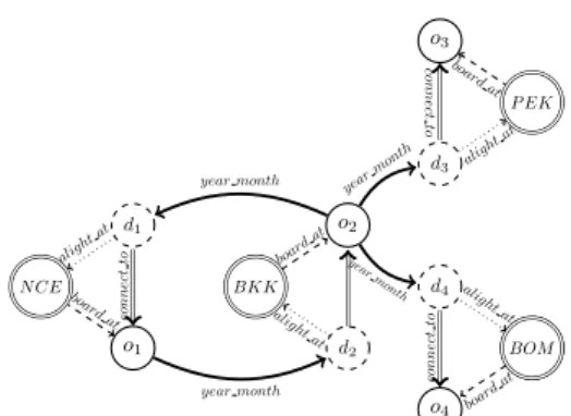
is one of the most popular graph databases where queries can easily be expressed through Cypher query language. Neo4j is used in many use cases, typically recommendation systems and complex networks like transportation network. In Neo4j, data are represented in nodes, relationships, and properties. Both nodes and relationships contain properties (Robinson et al., 2015). A relationship connects a pair of nodes, it has a direction, type, a start node, and an end node. In the company’s database, data are collected and queried monthly then it makes sense to create a relationship per period which is a month of the year. the rela-tionship represents flight information. We dis-pose of historical data about the last fifteen years. The current database used is a MongoDB database that stored data in a disconnected way. This database does not use a graph structure. There-fore, we opt for the graph database Neo4j as an-other alternative database to overcome the limits of the existing database (Neo4j, 2017). Neo4j uses a graph structure that regroups data and allows visualizing what happens in the network when creating a new route or deleting an ex-isting route. Furthermore, this graph database performed well on the graph traversal since our study is based on such algorithms (Holzschuher and Peinl, 2014). The graph database Neo4j of-fers the possibility to implement algorithms as user defined procedures to call in Cypher query. That is can be easy to use it by the final user. Indeed, Neo4j proposed APOC (Awesome Pro-cedures on Cypher) as stored proPro-cedures that re-group a list of procedures. Graph algorithms are part of these procedures namely some shortest path algorithms. Once the database is chosen, we proceed to model the graph. The model takes into account the transfer time. It is represented by a relationship in the graph. This technique is often used to model the information about trans-fer since it is important in computing shortest paths. The figure below illustrates the condensed graph in Neo4j. The graph contains four airports and four flight arcs. Nodes in thin style repre-sent departures (origin nodes), dashed nodes for arrival nodes (destination nodes). Double edge is transferring time meanwhile bold edges model flight time. Besides, dotted edges for arrivals and dashed edges for departures.
N CE d1 o1 BKK o2 d2 P EK o3 d3 BOM o4 d4 year month year month connect to alight at boar d at boar d at alight at alight at boar d at year month connect to year month boar d at alig htat connect to
Figure 1: Model of condensed flight network in Neo4j.
Thus, the condensed graph was generated for 1 year and has 33,901 nodes and 562,294 relation-ships.
5
PROBLEM FORMULATION
The flight radius problem consists in retriev-ing only relevant routes passretriev-ing through a spe-cific flight, and satisfying the regret function. The flight considered is represented by an arc (o, d) in the graph where o, d ∈ A. Then, we are interested in retrieving paths passing by the arc (o, d) that could be relevant regarding the regret defined for the time and cost criteria. In other words, travel-ing from o1∈ A to d1∈ A by passing through the arc (o, d) may be interesting if and only if the path {o1, .., o, d, .., d1} between o1 and d1 is accepted by the regret function. This function depends on the shortest path between o1 and d1. Let R be a Boolean regret function defined on paths of the graph G. Therefore, the problem consists in find-ing a maximal sub-graph, in terms of nodes, such that each node supports a path accepted by the regret function R.
Hence, the problem is formulated as follows:
Input a graph G = (V, E), the arc (o, d), and the
regret function R
Output a maximal subset E0 ⊆ E such that
G0= (V0, E0) is a sub-graph of G and that each node supports a path passing through the arc (o, d) accepted by the regret function.
In this paper, we use the regret function R to identify what paths are supported. Let’s define what the regret function R is. Let w(i, j) be the weight of the arc (i, j) and let l?(i, j) be the length of the shortest path from i to j. Let l(i, j) the length of a path passing through the arc (o, d), and let consider the following regret function de-fined for each criterion:
Where K ≥ 0. Each node must support at least a valid path by the regret function. Then, we are looking for retrieving paths that satisfied at least one criterion.
The flight radius problem consists in finding valid paths by the regret function R. These paths depend on finding shortest path. Most traditional path finding are based on shortest path finding:
l(i, j) ≥ l?(i, o) + w(o, d) + l?(d, j) (1) In other words, following the shortest path from i to o, passing by the arc (o, d), and then following the shortest path from d to j is always a valid path if it exists. The subpath from o to j of a valid path is also valid.
l?(i, o) + w(o, d) + l?(d, j) ≤ l?(i, j) + K
≤ l?(i, o) + l?(o, j) + K
w(o, d) + l?(d, j) ≤ l?(o, j) + K
Reciprocally, the subpath from i to d is valid. l?(i, o) + w(o, d) + l?(d, j) ≤ l?(i, j) + K
≤ l?(i, d) + l?(d, j) + K
l?(i, o) + w(o, d) ≤ l?(i, d) + K
Finally, the search can be restricted to shortest valid paths starting from o or ending at d.
Lemma 5.1. Let p be a valid path, all the nodes
belong to G0. For any shortest path p from o to j in G. If it passes through by d then it is a valid path and consequently j is going in the subgraph G0.
The subpath of the shortest path is also a shortest path (Ahuja et al., 1993). Consequently, nodes j represent set of nodes that support paths accepted by the regret function.
In the following, we focus on solving the part of finding the subpath from o to each vertex j.
6
SOLVING METHODS
6.1
A Query-Based Solution
In the earlier section, we proved that the search of valid paths can be restricted to find-ing valid shortest paths. The problem was solved in Cypher query using the algorithm BIDIRECTIONAL DIJKSTRA implemented in Neo4j as a procedure in APOC (Larsson, 2008). In
Neo4j, we use a parametrized query. The pa-rameters are: o code and d code to specify o and d, rel to identify type of relationship to traverse, criterion for time or cost, and K determines the regret.
The query described in 1 contains three ma-jor blocks. The first block of the query includes the first three lines. The MATCH clause is used to match the graph pattern which is the arc (o, d) using the supplied parameters. The second block contains the call of the algorithm. Then, the pro-cedure DIJKSTRA is called from the origin o to all other airports A in the graph in order to find the shortest path in terms of time, and finally gets the shortest paths from the destination d. The second WITH clause is to aggregate outputs of the first procedure. . Thus, calling the second proce-dure DIJKSTRA in the second block would execute the procedure for every row. The final block be-gins by the UNWIND clause to disaggregate previ-ous aggregate outputs. Meanwhile, the last WITH clause filters the set of paths according to the re-gret function.
6.2
An Algorithmic Solution
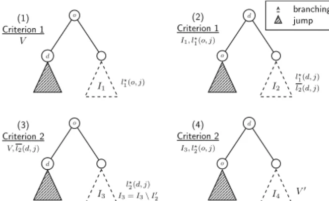
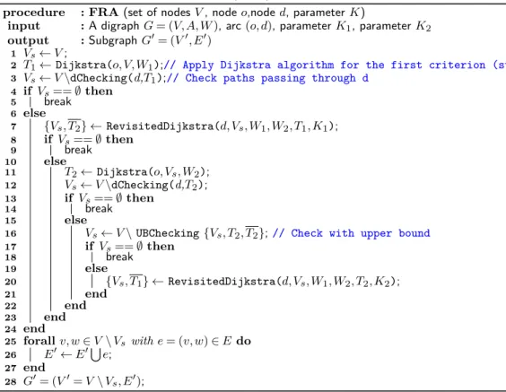
As the problem deals with two criteria, the algo-rithm starts by considering one criterion and then moves to the second one using at each step infor-mation from the previous step. The flight radius algorithm starts by computing the shortest path tree from o and checks if the arc (o, d) exists in the shortest path tree of o (lemma 5.1). After finding the shortest path tree (line 2 of Algorithm 1), we check valid shortest paths passed via d (line 3 of Algorithm 1). This step corresponds to the step (1) in Figure 2. The next step (2) is to compute the shortest path from d. In this step, we get two information: length of the shortest path for one criterion l?1(d, j) and an upper bound for the sec-ond criterionl2(d, j). Once we retrieve supported paths for the first criterion. We move to the sec-ond criterion and repeat the same process. The third step (step (3) in Figure 2) is more similar to the first. The another case where paths do not pass through d, we can use the upper bound com-puted in the previous step. We check if the regret function is satisfied for all nodes i ∈ Vs, set of non
supported nodes (line 16 of Algorithm 1). We ap-plied the same process for the remaining non sup-ported nodes to get the shortest path tree from d. To do this, we use a second algorithm, called RevisitedDijkstra. The algorithm represents the Dijkstra’s algorithm (Ahuja et al., 1993)
1 MATCH p=(Td:Destination)-[:ALIGHT_AT]->(o:Airport{code:{o_code}})-[:‘BOARD_AT‘]->(To:Origin)-[r ]->(d:Destination{code:{d_code}}),(A:Destination)
2 WHERE NOT A IN [d,Td] AND type(r) = {rel} 3 WITH r.duration_min-{K} AS LB,To,d,A
4 CALL apoc.algo.dijkstra(To,A,{rel}+’>|CONNECT_TO>’,{criterion}) YIELD path AS p1,weight AS w1 5 WITH DISTINCT A,collect(w1) AS W1,LB,d
6 CALL apoc.algo.dijkstra(d,A,{rel}+’>|CONNECT_TO>’,{criterion}) YIELD path AS p2, weight AS w2 7 UNWIND W1 AS w1
8 WITH w1-w2 AS diff,LB,A WHERE diff>=LB 9 RETURN DISTINCT A
Listing 1: CYPHER query
including the regret function. The algorithm at each iteration scans the node with the minimum label and then relax its neighbors. So, we check before if it satisfies the regret function otherwise we move to the next. Since all arc weights are nonnegative then Dijkstra’s algorithm finds the shortest path in order of increasing distance. For this reason, we use this manner to quickly remove non supported nodes. Figure 2 describes the steps of the flight radius algorithm.
(1) Criterion 1 V o d I1 l ? 1(o, j) (2) Criterion 1 I1, l? 1(o, j) d o I2 l? 1(d, j) l2(d, j) (3) Criterion 2 V, l2(d, j) o d I3 l? 2(d, j) I3= I3\ I0 2 (4) Criterion 2 I3, l? 2(o, j) d o I4 V0 branching jump
Figure 2: Flight radius algorithm steps.
7
EXPERIMENTS
In this section, we describe experiments on the flight radius problem. We start by evaluating the performance for solving the flight radius problem using a query. After that, we compare the result with those obtained using the algorithm in the case of one criterion. We measure information of the order of the output subgraph and the percent-age of nodes filtered with various value of the pa-rameter K. Those values are chosen randomly ac-cording to different statistic metrics. Specifically, we address the following questions: How sensi-tive is flight radius algorithm’s performance on the real graph to the choice of parameter K? How does an algorithm’s performance when adding a second criterion? How does the choice of one
pa-rameter K influence the order of the subgraph? All the experiments were led on a computer running on Ubuntu 16.04.2 with 32 GB of RAM and one Intel Core i7-3930K 3.20GHz processors (6 cores). The implementation is based on Neo4j and APOC version 3.2.0.1.
Test Instances. Tests on real-world data were
realized on the database of the company. To test the method based on a query, we use 6 instances for the problem, each one of them represents a flight with a different type of airport: hub & Spoke and using different value of the parameter K of one criterion. This parameter is chosen ac-cording to the minimum connection time M CT , and the median of each criterion. We compute the value of the parameter K according to the median, the first quartile, and the third quartile. In this way, we can measure the spread to describe the variability in each criterion with conjunction with the median as a measure of central tendency. In the case of criterion cost, K2is chosen indepen-dently to the minimum connection time M CT . Setting K to zero, for example, means that the subgraph contains all the shortest paths passing through the arc studied (o, d). On the contrary, setting K to a high value implies that the sub-graph contains all nodes of the condensed sub-graph. Note that the M CT is set to 120 minutes. Be-sides, we generate 100 instances that include for each pair of (OD) generated randomly, 10 tests with different classes of two criteria.
Problem with one criterion. Tests have been
run on existing flights between various airports in terms of degree. We apply the query for only one criterion since it takes a lot of time to solve the whole problem. We run tests on the time cri-terion. Table 1 gives the results of testing both methods. # nodes : the order of output sub-graph. Dur: flight duration of the arc studied, the parameter K1 fixed for each test, and the
Algorithm 1: Flight radius algorithm (FRA)
procedure : FRA (set of nodes V , node o,node d, parameter K)
input : A digraph G = (V, A, W ), arc (o, d), parameter K1, parameter K2
output : Subgraph G0= (V0, E0)
1 Vs← V ;
2 T1← Dijkstra(o, V, W1);// Apply Dijkstra algorithm for the first criterion (step (1))
3 Vs← V \dChecking(d,T1);// Check paths passing through d
4 if Vs== ∅ then 5 break 6 else 7 {Vs, T2} ← RevisitedDijkstra(d, Vs, W1, W2, T1, K1); 8 if Vs== ∅ then 9 break 10 else 11 T2← Dijkstra(o, Vs, W2); 12 Vs← V \dChecking(d,T2); 13 if Vs== ∅ then 14 break 15 else
16 Vs← V \ UBChecking {Vs, T2, T2};// Check with upper bound
17 if Vs== ∅ then 18 break 19 else 20 {Vs, T1} ← RevisitedDijkstra(d, Vs, W1, W2, T2, K2); 21 end 22 end 23 end 24 end 25 forall v, w ∈ V \ Vs with e = (v, w) ∈ E do 26 E0← E0S e; 27 end 28 G0= (V0= V \ Vs, E0);
percentage of nodes filtered. ExecT1 presents the running time of the first method whereas Ex-ect2 is for the second method. The running time of method based on a query is very important. Neo4j Implements bidirectional Dijkstra’s algo-rithm. So, the algorithm is repeated for each pair of nodes individually to find the shortest path from a node to all other nodes. Thus, many com-putations are repeated. However, our problem used the single-source shortest path algorithm. So, we are seeking to return the shortest path tree; that is, the shortest path from source to all nodes. But the result returned is a list of paths. That means, in terms of spatial complexity, the sum of the length of the n paths selected is bound by n2in the case of multiple runs of single-source shortest path algorithms rather than n paths in the case of three returned with n the number of nodes in the graph. The time complexity is O(n × (m + n log n)) as it runs multiple times as the order of the graph. In the worst case. The query runs in 57 minutes whereas, the algorithm takes only 2321 ms. Therefore, the algorithm out-performs the query.
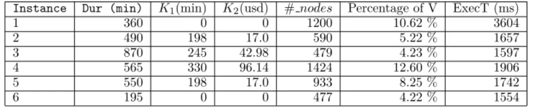
Problem with two criteria. Table 2 gives the
result of running the flight radius algorithm with two criteria. The percentage of supported nodes increases as we add a second criterion. Even with zero regret, the percentage is at least twice than the percentage in one criterion case. For the in-stance 1 and 6, the subgraph contains all short-est paths passing by these flights: (NCE, DXB) and (AMS,IST) for both criteria time and cost. In the instance 2, 3, and 4, the regret is chosen respectively to quartiles: Q1, Q2, and Q3.
Table 3 gives the average running time as a function of classes of parameter K1 and K2. The average running time increases slightly when both value increase. The algorithm runs in the best case when the parameter K1 is set to a value greater than the third quartile which represents 75 % of flight duration whereas K2 is setting to zero. In the worst case, the algorithm runs twice than in the best case. It is achieved when we swap both values. It comes back to the choice of the parameter K1 since it is computed in re-lation with the minimum connection time M CT . Then, the algorithm is influenced by the second parameter.
Table 1: Comparaison between two methods.
Instance Flight Dur (min) K1(min) # nodes Percentage of V ExecT1 (min) ExecT2 (ms)
1 NCE → DXB 360 0 287 2.5 % 53 2321 2 JFK → NCE 490 198 156 1.3 % 51 1127 3 CDG → SCL 870 245 56 0.49 % 55 696 4 LHR → ATL 565 330 771 6.82 % 51 786 5 FRA → PEK 550 198 416 3.68 % 53 736 6 AMS → IST 195 0 65 0.57 % 57 693
Table 2: Time needed to solve the flight radius problem with two criteria.
Instance Dur (min) K1(min) K2(usd) # nodes Percentage of V ExecT (ms)
1 360 0 0 1200 10.62 % 3604 2 490 198 17.0 590 5.22 % 1657 3 870 245 42.98 479 4.23 % 1597 4 565 330 96.14 1424 12.60 % 1906 5 550 198 17.0 933 8.25 % 1742 6 195 0 0 477 4.22 % 1554
Table 3: Average running time in function of regret classes. Class cost Class time 0 1 2 3 0 1573.6 1590.4 1657.2 2354.8 1 1783.2 1677.0 1759.4 2246.0 2 1877.8 2007.3 1928.1 2248.0 3 1367.0 2271.5 1484.1 1491.5
8
CONCLUSION
This work presents the flight radius problem. We formulated the problem as finding a maxi-mal subgraph, in terms of nodes, such that each node supports a valid path by the regret func-tion. To represent the regret function, we focused in the additive case. In the multiplicative case, the problem seems to be hard to simplify since the regret parameter K depends on the shortest path. Then, we presented two methods to solve the problem. Method using procedures of Neo4j the graph database where the condensed graph is stored and, the method based on a new algo-rithm that relies on Dijkstra algoalgo-rithm. Studied instances in this article were realized on the real-world network. The algorithm outperforms the query method and the choice of the parameter K influences the running time of the algorithm. Latter, we aim to test the algorithm on bench-marks graphs to test the performance when the topology changes. Also, we aim to test another shortest path algorithms which is Bellman-Ford since it takes O(nm) in the worst case and paths in flight network are characterized by small length in terms of number of arcs. Thus, we would like to compare its performance on the flight radius
problem compared to Dijkstra algorithm.
REFERENCES
Ahuja, R. K., Magnanti, T. L., and Orlin, J. B. (1993). Network flows: theory, algorithms, and
applications. Prentice hall.
Barnhart, C. and Cohn, A. (2004). Airline sched-ule planning: Accomplishments and opportuni-ties. Manufacturing & service operations
man-agement, 6(1):3–22.
Cherkassky, B. V., Goldberg, A. V., and Radzik, T. (1996). Shortest paths algorithms: Theory and experimental evaluation. Mathematical
program-ming, 73(2):129–174.
Hall, R. (2012). Handbook of transportation science, volume 23. Springer Science & Business Media. Holzschuher, F. and Peinl, R. (2014). Performance optimization for querying social network data. In EDBT/ICDT Workshops, pages 232–239. Jacobs, T. L., Garrow, L. A., Lohatepanont, M.,
Kop-pelman, F. S., Coldren, G. M., and Purnomo, H. (2012). Airline planning and schedule develop-ment. In Quantitative Problem Solving Methods
in the Airline Industry, pages 35–99. Springer.
Larsson, P. (2008). Analyzing and adapting graph algorithms for large persistent graphs. Master’s thesis.
Neo4j (2017). https://www.neo4j.com.
Rebetanety, A. (2006). Airline schedule planning
in-tegrated flight schedule design and product line design. University Karlsruhe (TH). PhD thesis.
Robinson, I., Webber, J., and Eifrem, E. (2015).
Graph databases: new opportunities for