HAL Id: hal-02620871
https://hal.inrae.fr/hal-02620871
Submitted on 26 May 2020
HAL is a multi-disciplinary open access archive for the deposit and dissemination of sci-entific research documents, whether they are pub-lished or not. The documents may come from teaching and research institutions in France or abroad, or from public or private research centers.
L’archive ouverte pluridisciplinaire HAL, est destinée au dépôt et à la diffusion de documents scientifiques de niveau recherche, publiés ou non, émanant des établissements d’enseignement et de recherche français ou étrangers, des laboratoires publics ou privés.
gravitropic sensitivities of plants combining an original
experimental device with model-assisted phenotyping:
Exploratory test of the method on three hardwood tree
species
Catherine Coutand, Boris Adam, Stéphane Ploquin, Bruno Moulia
To cite this version:
Catherine Coutand, Boris Adam, Stéphane Ploquin, Bruno Moulia. A method for the quantification of phototropic and gravitropic sensitivities of plants combining an original experimental device with model-assisted phenotyping: Exploratory test of the method on three hardwood tree species. PLoS ONE, Public Library of Science, 2019, 14 (1), pp.e0209973. �10.1371/journal.pone.0209973�. �hal-02620871�
A method for the quantification of
phototropic and gravitropic sensitivities of
plants combining an original experimental
device with model-assisted phenotyping:
Exploratory test of the method on three
hardwood tree species
Catherine CoutandID1*, Boris Adam2☯, Ste´phane Ploquin2☯, Bruno Moulia2
1 INRA, UR 1115 PSH, Avignon, France, 2 Universite´ Clermont Auvergne, INRA, PIAF, Clermont-Ferrand,
France
☯These authors contributed equally to this work.
*catherine.coutand@inra.fr
Abstract
Perception of inclination in the gravity field and perception of light direction are two important environmental signals implicated in the control of plant shape and habit. However, their quantitative study in light-grown plants remains a challenge. We present a novel method here to determine the sensitivities to gravitropism and phototropism. The method combines: (i) an original experimental device of isotropic light to disentangle gravitropic and phototropic plant responses; and (ii) model-assisted phenotyping using recent models of tropism per-ception—the AC model for gravitropism alone and the ArC model for gravitropism combined with phototropism. We first assessed the validity of the AC and ArC models on poplar, the classical species model for woody plants. We then tested the method on three woody spe-cies contrasted by their habit and tolerance to shade: poplar (Populus tremula*alba), oak (Quercus petraea) and beech (Fagus sylvatica). The method was found to be effective to quantitatively discriminate the tested species by their ratio of tropistic sensitivities. The method thus appears as an interesting tool to quantitatively determine tropistic sensitivities, a prerequisite for assessing the role of tropisms in the control of the variability of the habit and/or tolerance to shade of woody species in the future.
Introduction
Gravitropism and phototropism, the orientation of growth as a function of gravity and light, respectively, are two major processes implicated in the regulation of plant shape [1,2]. Their combination allows aerial organs to forage for light without losing mechanical stability [3]. This requirement is important for erect plants and obviously becomes crucial for trees in
a1111111111 a1111111111 a1111111111 a1111111111 a1111111111 OPEN ACCESS
Citation: Coutand C, Adam B, Ploquin S, Moulia B
(2019) A method for the quantification of phototropic and gravitropic sensitivities of plants combining an original experimental device with model-assisted phenotyping: Exploratory test of the method on three hardwood tree species. PLoS ONE 14(1): e0209973.https://doi.org/10.1371/ journal.pone.0209973
Editor: Christof Markus Aegerter, Universitat
Zurich, SWITZERLAND
Received: April 3, 2018 Accepted: December 14, 2018 Published: January 25, 2019
Copyright:© 2019 Coutand et al. This is an open access article distributed under the terms of the
Creative Commons Attribution License, which permits unrestricted use, distribution, and reproduction in any medium, provided the original author and source are credited.
Data Availability Statement: All relevant data are
within the paper and its Supporting Information files.
Funding: This work was supported by Agence
Nationale de la Recherche, ANR-11-BSV7-0012 TROPIC.
Competing interests: The authors have declared
which the shoot system is perennial and eventually very large. Moreover, differences in tree shape and the reaction to canopy opening [4] are often interpreted as resulting from different sensitivities to photo- and gravitropism. However, even if several molecular cross-talks between the gravitropic and phototropic pathways have been identified [5], very few quantita-tive studies have been conducted on the interaction between photo- and gravitropism and none provides numerical values of sensitivities to gravi- and phototropism for trees. This lack of data does not make it possible to compare the contribution of gravi- and phototropism between different tree species and thus prevents further advances in quantifying the contribu-tion of gravi- and phototropism in the control of tree shape (habit) variability.
When plants are subjected to gravitropism, they tend to reach the Gravitropic Set-Point Angle (GSA) [6]. However, the GSA can be modulated by several cues, e.g., light direction [7]. Galland extended the concept of GSA to the cases where both gravi- and phototropism are active: plants tend to reach a photogravitropic equilibrium angle (PEA) determined both by gravity field and light direction [8–9].
Further revisiting of Galland’s experiments by Moulia et al. using the formalizedArC
model [3] led to the definition of the Photo-Gravitropic Set-Point Angle (PGSA) and its quan-titative dependency on photo- and gravitropic sensitivities (but not on the initial tilting angle vs. gravity A0, in opposition to initial claims by Galland [8–9]). However, the estimation of the
PGSA and, finally, of the photo- and gravitropic sensitivities, have only been conducted so far in one set of experiments usingAvena coleoptile under continuous light [8,3].
The lack of knowledge about photo�gravi tropic interplay is even worse for trees. To our
knowledge, only two studies have investigated the phototropic movements of trees [10–11] and demonstrated that phototropism exists in their radially growing zones (woody stems). The gravitropic movement of tree axes (trunk or branch) has received more interest. Nevertheless, emphasis has been placed on the production of reaction wood, a specialized wood that acts as a motor for the tropistic movement of the woody stems and that has consequences on the qual-ity of wood in the lumber industry [12]. Consequently, no quantitative method is available to quantify tropistic tree sensitivities, which is a prerequisite for assessing the contribution and interaction of photo- and gravitropism in tree shape variability.
A quantitative study of the photo�gravi tropistic interactions in the driving of a tropistic movement faces two challenges:
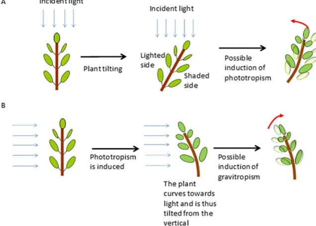
The first challenge is experimental. Indeed, gravitropism and phototropism are not easy to disentangle, at least on Earth ground at 1g. Indeed, as soon as a tree is tilted, one side of the stem is more shaded than the other, which can induce phototropism. Symmetrically, as soon as a vertical tree is lit unilaterally, it bends towards the light, which can trigger gravitropism (Fig 1). An obvious way to address this dilemma is through spatial experiments in micrograv-ity conditions [1] or on 3D clinostats. However, this is not really feasible with trees large enough to undergo significant secondary growth, and devices that would make it possible to fully avoid this dilemma on Earth are lacking.
The second challenge is that formalized modeling is required to analyze the interplay between growth, bending under self-weight and tropisms throughout the tropistic movement [12].
Starting with the pioneering model of Fournier et al. (1994) [13], down to the most recent ones by Coutand et al. [14–15], several models of tree tropisms have been designed [16–17]. All of them have combined: (i) a mechano-biological module of the perception-based driving of the differentiation of reaction wood; and (ii) a biomechanical module of the motor process to compute successive shapes of an axis though the mechanical actions of the differentiation of reaction wood and of the changes in the axis geometry and mass due to growth in girth [12]. This distinction between perception-based driving and motor processes is crucial: indeed,
differences in gravitropic sensitivity should not be confused with differences in motor efficien-cies (like the one that can be achieved with changes in trunk diameter of wood stiffness [18]). However, most of the research effort has focused on the motor module, taking into account: (i) spatial effects, i.e., asymmetric sections [18], and the heterogeneity of normal and tension wood; and (ii) time effects such as the effects of viscoelasticity and the maturation process [14– 15].
Consequently, in all these models, the perception-based driving module is very simple: local inclination from the vertical is perceived all along the trunk and reaction wood is pro-duced in a given cross-section as long as the tree has not reached the vertical position (hori-zontal cross-section). Models including such a basic perception-based driving module all failed to predict the anticipated decurving of the axis observed onPinus pinaster [13] and on
Populus [19], as well as in the coleoptile of wheatTriticum aestivum L. [20].
Recently, Bastien et al. concentrated on the perception-based driving processes during grav-itropism and gravgrav-itropism combined with phototropism, and provided two novel models of tropistic driving (AC model [20]) andArC model, [3]). They then assessed their models with experiments in which the motor process actuating the movements could be assumed to be non-limiting, mostly in herbs. TheAC model has been validated on 11 species, constituting a
sample of the phylogeny of land angiosperms. This made it possible to simulate the anticipated
Fig 1. Diagram explaining the interactions between gravitropism and phototropism in classical experiments dedicated to the study of gravitropism and phototropism. A: In classical experiments, a plant is tilted from the vertical in order to study gravitropism. In this
case, since the light is coming from the top, one side of the stem is shaded, which can induce a phototropic reaction. B: In classical experiments, a plant is lit unilaterally in order to study phototropism. Since the plant bends towards the unilateral light, the stem is curved and thus tilted, which can induce a possible counteractive movement due to gravitropism.
decurving process observed in pine [13], poplar [19], wheat and other species [20]. However, this validation was generally achieved on the steady-state shape of the plants and mostly for herbaceous species. The only woody plants that were assessed in [20] were two-year-old pop-lars (data from Coutand et al. [19]), but the assessment ofAC on poplar was less complete
since the achievement of a steady state was not fully assessed. TheArC model has only been
assessed in one herbaceous species,Avena sativa L (and only on the coleoptile of its seedling).
In this work, we propose an original method to compute gravitropic and phototropic sensi-tivities of trees. Two dedicated experimental devices were designed and built expressly for the development of this method. One, fully original, was dedicated to disentangling gravitropism from phototropism: it makes it possible to tilt young trees in an isotropic light environment, thus triggering the gravitropic response alone. The other is more classical and combines plant tilting and unilateral lightening to study the interaction between gravi- and phototropism. In both set-ups, kinematics of tropistic movements were recorded and fully quantified.
Using these experimental set-ups, we first assessed the validity of theAC and ArC models
for young trees. We then used model-assisted phenotyping withAC and ArC models to
deter-mine gravitropic and phototropic sensitivities of tree seedlings. In this exploratory work, the method was tested on three hardwood species that exhibited different behavior to light and type of growth: poplar (pioneer species, fast growth), oak (hemi-tolerance to shade, rhythmic growth) [21], and beech (high tolerance to shade, slow growth) [22] in order to illustrate the ability of the method to discriminate the three species on the basis of their tropistic
sensitivities.
Material and methods
Plants
Very young trees at a stage in which the shoot is about 30- to 50-cm-long were chosen because at this stage, the motor process is likely to be non-limiting and gravi- and photogravitropic equilibrium can be reached within a few weeks [13,19].
Poplar: Young poplars (Populus tremula × alba cv 717 1B4) were obtained by in vitro
micropropagation and planted in individual 5-L pots filled with loam after progressive accli-mation. Trees were grown in a growth chamber (L/D 16 h/8 h at 24˚C/20˚C with RH 60± 10%). Two months after micropropagation, the poplars were ready to be used in experi-ments; stems were at least 35-cm high at this stage.
Beech and oak: One-year-old beech and oak seedlings were purchased in a commercial nursery and planted in individual pots filled with 1/3 black peat and 2/3 local “Limagne” soil in autumn 2013 and 2014 and grown in a greenhouse. Watering was ensured on immersion tables. Beech seedlings were protected from direct sun by 55% shade cloth (Puteaux SA, Les Clayes sous Bois, France).
Experimental devices to study tropistic responses. We designed and constructed novel
experimental devices called “isotropic light spheres” to disentangle gravitropism and phototro-pism. These spherical growth cabinets allowed young trees to be grown and tilted in an isotro-pic light environment in such a way that photosynthesis and growth are ensured by light, gravitropism is triggered by tilting the tree, but no phototropic signal is triggered because the lighting is the same from any direction around the tree (isotropy). This device thus made it possible to study the gravitropic response alone during long-term experiments under light conditions.
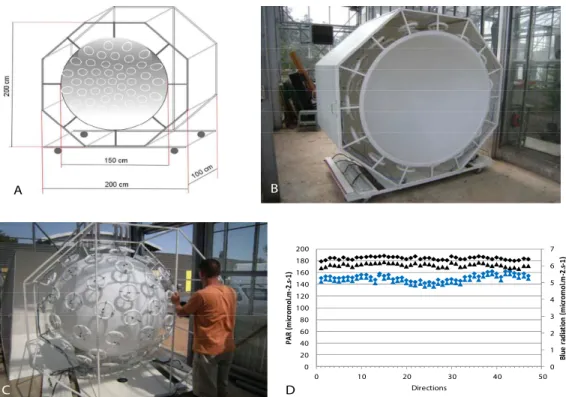
Two spherical growth cabinets with isotropic light were constructed: each device makes it possible to tilt a young tree in an isotropic light environment. Each sphere was composed of two 1.5-m-diameter hemispheres of transparent polymethyl methacrylate mounted on two
specifically designed (INRA, Nancy, France) hexagonal metallic rolling structures (Fig 2A). The inside of each hemisphere was painted white by a bodywork company (Carrosserie David et Fils, Clermont-Ferrand, France) to obtain a homogeneous diffuse light transmission. Each hemisphere was equipped with 46 circular fluorescent tubes (OSRAM, FC 22W/865) placed according to Den Dulk’s ‘TURTLE’ pattern [23]. These neon tubes were chosen because they provided a quality of light that is the closest to sunlight (see spectrum inS1A Fig). The neon tubes were fixed to the outside of the sphere (Fig 2B). In order to maintain the maximum amount of light provided by the neon tubes, reflecting shiny metallic plates were set around each sphere (Fig 2C). Because of the heat produced by the system, a controlled mobile cooling system (Blyss WAP 267EC) was added to each sphere to maintain the temperature at approxi-mately 25˚C in the sphere during the lighted periods.
The homogeneity of the emitted radiation of each sphere in terms of blue and photosyn-thetically-active radiation (PAR) was assessed using a spectrometer (FieldSpec Pro, Analytical Spectral Devices, Inc., Boulder, CO, USA) set on a pan-tilt robot (Biclops P/T, TrackLabs, Webster, TX, USA) to measure radiation in 46 directions. PAR and blue radiation were homogenous within the 46 directions (Fig 2D). PAR was approximately 180 W.m-2and the blue radiation fluence rate was approximately 5μmol.m-2.s-1.
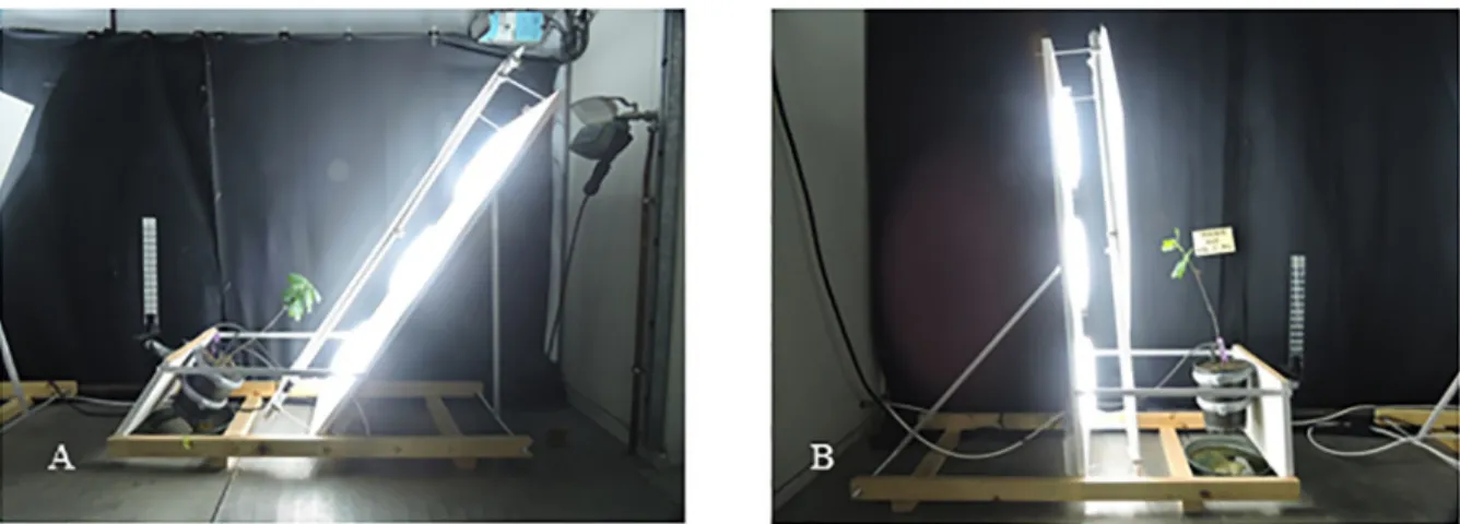
We also designed lateral light devices to study combined gravitropism and phototropism: The device providing anisotropic lateral light together with plant tilting is based on a panto-graphic system that makes it possible to choose the same tilting angle for the plant and the board where a light source was mounted (35˚, 25˚, 15˚, 5˚ (Fig 3A and 3B)). The light source was composed of three circular fluorescent tubes (OSRAM FC 865) set in a row on a white
Fig 2. Isotropic light device. A: 3D quoted scheme of the isotropic light device. B: View of one hemisphere showing the
turtle pattern of circular neon tubes at the periphery of the white plastic hemisphere. C: View of one hemisphere covered with metallic plates to concentrate the lighting towards the inside of the hemisphere. D: Measurements of PAR and blue radiation in the two spheres in 46 directions with an optic fiber mounted on a robot set in the center of the sphere. Black symbols: PAR; blue symbols: blue radiation.
board. These neon tubes were chosen because they provided the quality of light the closest to that of sunlight (the spectrum is available onS1 Fig).
Lighting power could be controlled by changing the neon tubes (55, 40 and 22 watts). A fourth light power of 15W was obtained by setting a neutral filter (216 LEE FILTERS White Diffusion 15FT) in front of 22W neon tubes. The light source came from the lower side of the trees in order to better qualify the tree movements either upward towards the vertical (gravi-tropism) or downward towards the light source (photo(gravi-tropism). Depending on the size of the plant studied, the three neon tubes could be turned on independently to ensure that the light came only from the lower side of the tilted tree. In our experiments, two neon tubes were switched on for beech and oak. For poplar, since they greatly elongated during their tropistic movements until equilibrium, two, and then very rapidly (two weeks after the beginning of the experiment) three neon tubes were switched on, so that the entire plant remained laterally lit throughout the experiment.
To obtain an exact measurement of light fluence rates reaching the plant stem on the aniso-tropic light devices, measurements were performed with a ceptometer (AccuPAR LP-80, Deca-gon Devices) set parallel to the board where light sources were fixed. Measurements were made when the board containing the light sources was tilted at different angles: 0˚, 5˚, 15˚, 25˚ and 35˚ from the vertical (S2 Fig). The ceptometer made it possible to measure the photosyn-thetically-active radiation (PAR). Additional measurements with a spectrophotometer (Field-Spec Pro, Analytical (Field-Spectral Devices, Inc., Boulder, CO, USA) allowed us to obtain the spectrum of each type of neon tube (S1 Fig), in particular, blue radiation, the main active one for phototropism. A very similar level of PAR and blue radiation was exhibited by 40W and 50W neon tubes. Spectra values of fluence rates in the PAR and in the blue radiation were computed by integration for every tilting angle and type of neon tube. On the basis of these computations of PAR and blue fluence rates, fluence rates of blue radiation included in the PAR measured by the ceptometer were computed (S1 Table). PAR ranged from 50 to 160μmol.m-2.s-1and blue radiation ranged from 6 to 20μmol.m-2.s-1.
PAR values and blue radiation values are given inS1 Table.
To provide full control of the temperature and humidity, the anisotropic light devices were placed in growth chambers. The walls of the growth chambers were covered with black
Fig 3. Side views of the anisotropic light device installed in a growth chamber. A: Young oak is installed on the anisotropic light device
tilted 35˚ from the vertical. B: Young oak is installed on the anisotropic light device tilted 5˚ from the vertical. The walls of the growth chamber were covered with black curtains in order to avoid light reflection.
curtains to avoid reflection of light on the walls. Four anisotropic light devices could be installed in a growth chamber at the same time and two similar growth chambers were avail-able at the same time, making it possible to experiment on eight plants simultaneously.
We monitored growth and tropistic movements. Stem diameters were measured weekly using a caliper. Secondary growth was expressed as the average daily diameter growth rate measured at 10 cm from the stem base. Tropistic movements were recorded every 2–3 days by photographs until equilibrium was reached (no detectable movement for two weeks). In each treatment, a picture of the main stem was taken with a digital camera (CASIO, Exilim EX-F1). In order to obtain the scale within each picture, a gradual test card was fixed on each tilting device in the plane of the plant and set at the vertical. For each picture, particular care was taken to align the vertical bars of the grid of the camera screen with the vertical position using the gradual test card. The shape of the main stem on each picture was recorded by digitizing with ImageJ software (NIH) in order to obtain the coordinates (x,y) of each point along the stem. Sets of digitized points give the shape of each seedling stem. Two successive digitized points were approximately 0.5 cm apart.
A preliminary work was performed to assess experiment length: one young tree was tilted 35˚ on the isotropic light device and a very similar one was tilted on the anisotropic light device. Stem movements were then recorded until a steady-state shape was reached (no move-ment detected for two weeks).
In poplar seedlings, the fast growing species, the time of the experiment necessary to reach the steady state was approximately four weeks. In oak and beech, which are classified as slow growing species, the required time was found to be about two months.
Treatments. Study of gravitropism alone: Young poplar, beech and oak were tilted in an
isotropic light environment (one tree per device in each experiment) in controlled conditions (25˚C/22˚C, 16 h L/8 h D). Two replicates were performed per species.
Study of combined gravitropism and phototropism: Young poplar, beech and oak were tilted in an anisotropic light environment (one tree per anisotropic light device in each experiment) in controlled conditions (25˚C/22˚C, 16 h L/8 h D). Each species was submit-ted to a cross-plot design of gravi- and phototropic stimuli (treatments) with four tilting angles (5˚, 15˚, 25˚ and 35˚) and four neon tube powers (15W, 22W, 40W and 55W). Because this study focused on methodological feasibility assessment and the experiments were long, all 16 treatments were conducted in only one replicate. Nevertheless, the four tilt-ing angles under the 40W neon lighttilt-ing were replicated for poplar and oak, but not for beech due to experimental hazards. For this last species, only the 35˚ tilting treatment (which induced photogravitropic movement; seeResultssection) could be repeated once with 40W neon tubes. Note additionally that the 55W neon tubes provided values of PAR and blue radiation similar to those of the 40W neon tubes (so that the two treatments are in fact almost replicates).
Anatomical study. For tilted beech seedlings, detection of tension wood was performed
following a classical double-staining procedure with safranin and astra blue (dx.doi.org/10. 17504/protocols.io.rdmd246).
AC and ArC models used to determine tropistic sensitivities
AC model (perception of gravitropism). In theAC model of perception-based driving,
the gravitropic movement was found to be directly driven by the perception of both local incli-nation (gravitropism) and of curvature induced by the tropistic movement (proprioception) [20]. More accurately, during the gravitropic movement, at any timet, the curvature rate of
perceptions of local inclination (A(s,t)) and of the curvature (C(s,t)):
dCðs;tÞ
dt ¼ bAðs;tÞþ gCðs;tÞ ð1Þ
where parametersβ and γ are the sensitivity to gravitropism and sensitivity to proprioception, respectively.
Note that if the model is linear in its parameters of gravi- and proprioceptive sensitivities, the differential equation is not linear because A is the spatial integral of C.
This study also demonstrated that the gravitropic equilibrium can only be reached through the balance between graviperception and proprioception. Indeed, the model predicts the angle of the stem from the vertical, at a location s along the stem at the steady state (GSA), as:
Aðs;tÞ¼A0exp bs
g ð2Þ
Dimensional analysis ofEq (1)leads to the definition of the dimensionless parameter B, called the Balance number:
B ¼b
gL0 ð3Þ
whereL0is the initial length of the part of the stem that is active in the tropistic motion. B is thus the ratio of the gravi- and proprioceptive sensitivities, scaled to the active size of the plant (the size of the zone of the stem that is both sensing and actuating the gravitropism). B is an essential parameter controlling both the final shape of the shoot and its overall gravitro-pic dynamics [20]. For the same trunk length, the shape of the trunk at gravitrogravitro-pic equilibrium displays more or less concentrated and intense curving depending on the ratio of sensitivity to gravitropism and sensitivity to proprioception. On the basis ofEq 2, the value of B can be esti-mated through the fit of the field of local inclination along the trunk at gravitropic equilibrium by an exponential, together with the length of the trunk. Note that B can also be determined by fittingEq 1of theAC model during the tropistic movement, but according to [20], estimating B on the steady-state shape was easier because angle measurements are much less noisy than those of curvature that involve a spatial derivative of the angle, thus enhancing the noise. How-ever, such measurements and estimations of B for a pure gravitropic stimulus have only been conducted in primary growing zones of herbaceous plants grown in the dark [20].
ArC model (perception of combined gravitropism and phototropism). Bastien et al. extended theAC model to include phototropism, leading to the ArC model [3]. TheArC
model maintains the same characteristics of theAC model for gravitropism but also integrates
the perception of light direction (phototropism) by including a sensitivity to the angle (App) between the apex direction and the light direction. At photogravitropic equilibrium, the top of the plant is set at the PhotoGravitropic Setpoint Angle (PGSA), also designated Ar (for resul-tant angle) for convenience in theArC model.
In theArC model, during the photogravitropic movement, at any time t and position s
along the stem, the curvature rate of the stem is driven by the sum of three perceptions: tion of local inclination (gravitropism), perception of curvature (proprioception) and percep-tion of the angle between the apex and the light direcpercep-tion (phototropism). The model has three parameters: the first two are shared with theAC model (β—the sensitivity to gravitropism-; γ
equation of the model is the following:
dCðs;tÞ
dt ¼ bAðs;tÞþ gCðs;tÞþvðAðL;tÞ ApÞ ð4Þ where L is total stem length,A(s,t) is the local inclination, C(s,t) is the curvature, A(L,t) is the
inclination of the tip of the stem (s = L), andAp is the inclination of light from the vertical. A (L,t)—Ap is thus the angle between the apex and the light direction (App).
Dimensional analysis of the equations of theArC model leads to two dimensionless
num-bers, B and M: B ¼b gL0 ð5Þ and M ¼b n ð6Þ
Thus, theArC model adds a second character measured by the dimensionless number M to
the balance number B, the “Motion-pointing number”, which is the ratio between gravi- and phototropic sensitivities. It was in fact shown that for a given angle of incoming light from the vertical (Ap), the Photo-Gravitropic Setpoint Angle Ar only depends on M:
Ar Ap¼
1
1 þM ð7Þ
Together B and M fully control the tropistic dynamics and the final steady-state shape of the shoot at photo-gravitropic equilibrium. They are thus sufficient for a complete quantitative phenotyping of the sensitivity balance involved in driving the tropistic movement resulting from the interaction between photo- and gravitropism (also involving proprioception).
Similarly to the estimation of B using theAC model, M can be determined using the ArC
model equations (model–assisted phenotyping) in two ways: (i) by statistical fitting of the modelEq (4)on an experimental dataset recording the photogravitropic movement vs. time (curvature rate, local inclination, curvature, angle of the apex with incident light) to estimate theβ and ν parameter values; and (ii) by computing the ratio Ar/Ap from the measurement of Ar on the photograph of the stem at PGSA and the direction of the incoming light from the vertical (Ap).
Note that in addition to M, B can also be determined using the equation of theArC model
during tropistic movement, knowingβ and γ parameter values. Bastien et al. [3] did not retain this approach for two reasons: (i) parameter estimates on the curvature dynamics are noisier; and (ii) estimating the three sensitivities at once using a single equation and a single experi-ment is prone to statistical biases linked to parameter correlations and compensations. There-fore, they suggested a two-step phenotyping: phenotyping of B using theAC model on purely
gravitropic experiments, and then phenotyping of M using theArC model on
photo-gravitro-pic experiments.
Note finally that the amount of incoming light intensity can affect the value of M and, in theArC model, the function can be either logarithmic (Fechner’s law [8–9]) or a power func-tion (Steven’s law [3]).
TheArC model was assessed [3] using the detailed experimental data produced by Galland onAvena coleoptiles [8–9]. It was shown that Ar is determined simply by the relative sensitivi-ties to gravitropism and phototropism through the number M and the light direction from the
vertical (Ap) but not by the initial tilting angle of the tree from the vertical, as predicted by the
ArC model and contrary to the initial claim by Galland [3]. Additionally, photogravitropic equilibrium Ar was found to be dependent on the light fluence rate following a power law function, at least inAvena coleoptiles. However, the ArC model has not yet been assessed on
data from woody species.
Statistical assessment of the
AC and ArC models with data of tropistic
movements in poplar
TheAC and ArC models were tested on poplar data to estimate values of their parameters of
sensitivities to gravitropism (β), proprioception (γ) (AC model), gravitropism (β), propriocep-tion (γ) and sensitivity to light direcpropriocep-tion (ν) (ArC model). To do this, the rate of curvature was considered as the variable to be explained, and local inclination and curvature were the expli-cative variables for theAC model; inclination, curvature, and angle between the apex and the
light were the explicative variables for theArC model. AC and ArC models are linear in their
parameters so they were tested through multivariate linear regression (LinearModel.fit proce-dure of Matlab).β and γ parameters were computed for trees for which only gravitropism was triggered, andβ,γ and ν were determined for each tree for which both gravi- and phototropism were triggered. To assess the values of parameters of theAC and ArC models, statistics with
type III errors were used because predictive variables could be correlated. Indeed, the curva-ture field is obtained from spatial derivatives of the local inclination field and incident light is correlated with the inclination of the pot so that the angle between the apex and the incident light might be correlated with the local inclination.
Input data for running a statistical multivariate linear fitting of theAC model
(gravi-tropism only). On the basis of datasets of digitized points of stem shapes, the curvature field
was computed for each shape of each stem following the Matlab procedure detailed in [19]. Briefly, each stem shape was first fitted by a smoothing spline. Then, first and second deriva-tives of the spline function (P(x)) were calculated. The local curvature at any material point (i)
located at a distance (s) from the stem base was then computed by the following formula:
Ci ¼ d2Pðx iÞ=dx 2 ð1 þ ðdPðxiÞ=dxÞ 2 Þ3=2 ð8Þ
The local inclination field of each shape of each stem was computed by spatial integration of the curvature field and the initial tilting angle. Note that in this study, 0˚ refers to the vertical position and angles are counted positively in the counter-clock direction.
Both curvature and local inclination are the explicative variables of the linear regression analysis.
The fields of curvature rate along each stem were computed from computed fields of curva-ture and the time elapsed between two successive photos. The curvacurva-ture rate was the variable to be explained in the linear regression analysis. Computations were made considering the dis-placement of material points due to elongation in the upper part of the stem during the tropis-tic movement [24] using REGR measurements, via the classical technique of ink marks [25– 26] on another set of seedlings.
Input data for running a statistical multivariate linear fitting of theArC model
(com-bined gravitropism and phototropism). In addition to the input data for theAC model, the
inclination at the tip of each shape of each tree was extracted from the field of local inclination and the angle (App) between the apex (local inclination at the tip of each stem shape), and the direction of light from the vertical (Ap) was computed (S3 Fig). Since the light source was fixed on a board that was tilted at the same angle as the angle imposed on the plant pot, the
angle of light with the vertical (Ap) is directly computed from the inclination imposed to the plant pot (α) by: Ap=−90 + α.
For poplar, M was then computed from values of sensitivitiesβ and ν obtained (Eq 4) with a statistical multivariate linear model run with data from the curvature rate kinetics (variable to be explained) and local inclination, curvature and angle between the apex and the light direction (explicative variables).
Note that the values of parameters given by statistics also made it possible to compute the parameter B, following the same procedure as with gravitropism data alone, usingEq 3.
The regressions analyses provided satisfactory results concerning the statistical significance of the models so that we computed parameter B for every tree using theAC model, and
param-eters B and M using theArC model for most of the trees tested for combined gravi- and
phototropism.
Computation of B and M parameters from the final shape with
AC and ArC
model equations at steady state
Computation of parameter B from the equation of theAC model at steady state. For
computing parameter B, the local inclination field along each stem vs. the curvilinear abscissa (position along the stem from the stem base) at gravitropic equilibrium was fitted with an exponential function followingEq 2. The value of parameter a of the fit provided the inclina-tion at the stem base, and the value of b of the fit gave the ratioβ/γ. The value of B was then obtained usingEq 3. Note that this way to determine B could only be used with data obtained using the isotropic light device (gravitropism alone).
Computation of M parameters from the equation of theArC model at steady state. To
determine M, Ar was measured at photogravitropic equilibrium (PGSA) in the combined photo- and gravitropism experiments. Ar was measured at the top of the stem (below the annual shoot for beech). The value of M was then computed for each seedling usingEq 7
Effect of light intensity on M parameter values
To assess the dependency of M vs. blue light intensity, M was plotted as a function of the blue light fluence rate (the relevant waveband for phototropism) and either fitted with a power function (Steven’s law), or fitted with a logarithmic function (Fechner’s law).
Comparison of the estimates of B and M parameters from kinetics and
from final shape at steady state
For poplars, B and M parameters were computed by two means:
1. The values of parameters were first computed from the values of sensitivities (β,γ,ν) obtained by linear regression using Eqs3,4and7(model parameter method), only when theArC model parameters were statistically significant at the level of 5% and when β and γ
and whenβ and ν had the same signs (otherwise leading to negative values of B and M, respectively).
2. The values of parameters B and M were also computed from the stem shapes at gravi- and photogravitropic equilibrium (“final shape method”)
Values of both B and M obtained from the two methods (“final shape method” or “model parameter method”) were compared. For B, the two methods were compared by a pairwise t test for both the radially growing zone and for the whole stem, thereby providing a complete test of theAC model.
Results
Growth and characteristics of tropistic movements of each species
Growth. All light conditions tested in this study were sufficient to ensure growth in girth
for the three species studied (S2 Table). As expected, poplar exhibited the highest growth rate, which was about five times more than for oak and beech. Oak grew slightly faster than beech.
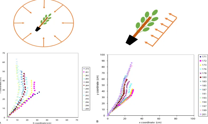
Tropistic movements. Poplar: When subjected to tilting in an isotropic environment
(gravitropism alone), the young poplar stem uprighted itself until a large part of the stem reached the vertical position, leading to a steady state (Fig 4A). When they were subjected to tilting in an anisotropic environment, the stem uprighted itself and then stabilized at an angle (Ar) different from the vertical (Fig 4B). The photogravitropic movement was continuous until equilibrium (PGSA).
Oak: When oak trees are subjected to tilting in an isotropic light environment (gravitropism alone), stems stabilized with the top of the stem back to the vertical position (Fig 5A). When the annual shoot elongated while the seedling was tilted in an anisotropic environment, the stem bent towards the light (Fig 5B). However, when no annual shoot elongated (case of three seedlings among twenty seedlings) while the seedling was tilted in an anisotropic light environ-ment, the stem uprighted itself as if the seedling was subjected to tilting alone (Fig 5C). Since our focus in this study was on photo�gravitropic interactions (and not on the location of
pho-totropic sensing), these latter cases were not considered in the following.
Beech: When beech seedlings were tilted at various angles from the vertical in an isotropic light environment, two cases were observed. When the tilting angle was smaller than 20˚, no movement was observed. When the tilting angle was larger than 25˚, the stem (except for the annual shoot) uprighted but stabilized at an angle of about 20˚ from the vertical (Fig 6). When beech seedlings were tilted at various angles from the vertical in an anisotropic light environ-ment, two cases were observed. When the tilting angle was smaller than 20˚, no movement was observed; when the tilting angle was larger than 20˚, the stem (except for the annual shoot) uprighted but stabilized at an angle larger than 20˚ from the vertical (Fig 7). In the fol-lowing, we focused on the cases where tropistic movements could be observed.
Assessment of the
AC and ArC models with the poplar datasets
AC model. β, γ parameter values of the AC model were determined by linear regression on tropistic kinematics: For each of the two poplar seedlings, results and statistics of the regres-sion analysis are given inS3 Table.
For the radially growing zone, the linear model was statistically highly significant, but it only explained from 20% to 31% of the variability of the curvature rate. Values of both parame-tersβ and γ were highly significant. B values were then obtained for stem 1(B = 2.4) and for stem 2 (B = 2.98) (Table 1, “model parameter method” column).
Considering regression on the whole stem, the model was also highly significant.β and γ were also computed from results of linear regression with data on the whole stems (annual shoot included). This led to B = 2.12 for stem 1, and B = 3.05 for stem 2 (Table 2, “model parameter method” column).
Values of the B parameter were determined on the stem shape at gravitropic equilibrium: For each of the two poplar seedlings, in order to determine B (Eq 3), the local inclination at gravitropic equilibrium (GSA) vs. the position along the stem (curvilinear abscissa) was fitted with an exponential function (S4andS5Figs). Because the steady state shape does not depend on the motor efficiency (but just on the driving), the values of B were computed for data con-cerning the radially growing zone of the stems (like before) but also from data concon-cerning the
whole stems in order to assess if similar driving could operate on the primary and secondary growth zone.
Analysis of the radially growing zone of the stems led to B = 2.26 for seedling 1 and B = 2.21 for seedling (Table 1, “final shape method” column), whereas the analysis of the whole stems led to B = 1.94 for seedling 1 and B = 2.01 for seedling 2 (Table 2, “final shape method” column).
Test of consistency of the two methods for estimating the values of B was performed: Parameter values obtained by the two methods (“model parameter method” and”final shape method”) for the two stems did not significantly differ at the level of 5% for the part undergo-ing radial growth (P value = 0.33) or for the whole stem (P-value = 0.39), regardless of the method used.
ArC model. β, γ and ν parameter values of the ArC model were determined by linear regression on the tropistic kinematics:Values of parameters (β,γ and ν) and results of the regression statistics of theArC model are given inS4 Table. Linear regression of theArC
model was highly significant for all trees and the parameter values were significant for most of the regressions. However, one of the values of the three parameters was not statistically signifi-cant at the 5% confidence level for 20% of the trees.
Test of consistency of the estimation of B from theArC and AC models was performed: The
parameters of theArC model fitted on the data of the anisotropic experiments led to an average
value of B = 0.7. B values computed from the parameters of modelAC obtained from isotropic
Fig 4. Successive shapes of poplar stems subjected to tilting in an isotropic light environment or in an anisotropic light environment. A: Isotropic light
environment: the stem tends to be vertical at steady state. B: Anisotropic light environment: the stem remains inclined at steady state.
Fig 5. Examples of tropistic movement of oak seedlings subjected to tilting in an isotropic or anisotropic light environment. A: Case of oak seedling subjected to tilting in an isotropic environment: the stem stabilized with the top
of the stem back to the vertical. B: Case of oak seedling subjected to tilting in an anisotropic light environment and for which an annual shoot elongated during treatment: the stem stabilized towards light. C: Case of oak seedling subjected to tilting in an anisotropic light environment and for which no annual shoot elongated during treatment: the stem uprighted itself and stabilized around the vertical position.
Fig 6. Shapes of beech trees just after tilting and at equilibrium, in an isotropic light environment. A: Pots were
tilted 20˚ from the vertical. No movement could be detected except at the top of the stem (annual shoot), which was tilted more than 20˚. B: Photos of anatomical double-stained transversal sections of the stem: B1: Section cut between 0 and 10 cm from the stem base: no reaction wood can be detected; B2: Section cut in the upper part of the stem below the annual shoot: a sector of reaction wood can be detected (crescent stained blue). C: Pots were titled 45˚ from the vertical. Tree exhibited a visible upward movement. D: Photo of anatomical double-stained transversal sections of the stem. D1: Section cut between 0 and 10 cm from the stem base: a sector of reaction wood can be detected. D2: Section cut in the upper part of the stem below the annual shoot: a sector of reaction wood can be detected. E: Pot was tilted 20˚ from the vertical for two weeks. The shapes of the stem during the two weeks of tilting are represented; dates are indicated on the graph (Julian days). Almost no movement can be detected. F: The tree was first tilting 20˚ from the vertical (shown on E) and then the tilting was increased to 45˚. Stem shapes until gravitropic equilibrium are presented at the different dates indicated on the graph. The stem uprighted itself.
Fig 7. Beech seedling shapes just after tilting and at photogravitropic equilibrium in an anisotropic light environment, for different values of initial tilting. Initial shape (blue symbols) and shape at photogravitropic equilibrium (red symbols) obtained by photo
digitizing with Image J. Dates of photos are indicated on the graph (Julian days). A, B: Pots were tilted 5˚ and 15˚ from the vertical, respectively. No movement could be detected. C, D: Pots were tilted 25˚ from the vertical. Tree exhibited no movement (C), or movement (D). E, F: Pots were tilted 35˚ from the vertical. Trees exhibited a visible movement spread throughout the stem length.
light experiments were around 2. The use of theArC model parameters thus led to B values
about twice as small as theAC model parameters.
A consistency test of the methods for estimating the values of M using theArC model in
kinetics or at steady state was performed: The M values obtained from linear regression of the
ArC model with kinetics data of photogravitropic movements and those obtained from
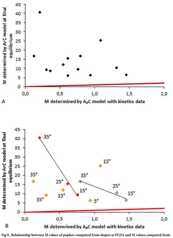
pheno-typing stem shape at steady state (PGSA) with theArC model were compared (Fig 8).
When considering the whole dataset (Fig 8A), several remarks can be made. First, the values of M determined from final shapes are always higher than the values of M determined from kinematics data. To find some possible explanations for this discrepancy, we examined the relationship by clustering the data by light fluence rates in the treatments (Fig 8B). Doing so, the correlation coefficients were much higher than the ones obtained using the whole dataset with no clustering. As a general trend, the data obtained for a given lighting for small tilting treatments were the closest to the line 1:1. This result stems from the fact that when designing theArC model, the sine law for both the angular response vs. gravity and vs. the light sources
has been simplified to the first (linear) term of the sine Taylor series (see, for example, Equa-tions. 4 and 11 in [3]). This simplification is obviously only accurate for small angles. It is therefore almost not biased concerning the shape prediction by the model in the steady-state form (in general, the angles are moderate) or at the end of the tropistic kinematics, but the bias is greater at the beginning of the kinematics when the angles vs. gravity and/or the light source are high.
As a conclusion for these results on poplar, the determination of B by theAC model
param-eter method or by the final shape method provided good results, indicating that theAC model
is validated when considering data concerning the pure gravitropic response of the trees. The determination of B by theArC model parameters led to an underestimation of B, very probably
due to our tilting device in anisotropic light (seeDiscussionsection).
The determination of M by theArC model parameters obtained by the model parameter
method and by the final shape method led to a four-fold discrepancy. This discrepancy can be
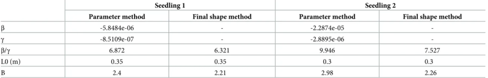
Table 1. Values of gravitropic (β) and proprioceptive (γ) sensitivities (SI unit) and B determined with AC model phenotyping with the “parameter model method” and the “final shape method” in the radially growing zone of the stem (i.e., stem with the exception of the annual shoot).
Seedling 1 Seedling 2
Parameter method Final shape method Parameter method Final shape method
β -5.8484e-06 - -2.2874e-05 -γ -8.5109e-07 - -2.8895e-06 -β/γ 6.872 6.321 9.946 7.527 L0 (m) 0.35 0.35 0.3 0.3 B 2.4 2.21 2.98 2.26 https://doi.org/10.1371/journal.pone.0209973.t001
Table 2. Values of gravitropic (β) and proprioceptive (γ) sensitivities (SI unit) and B determined with AC model phenotyping with the “parameter model method” and the “final shape method”, on the whole stem.
Seedling 1 Seedling 2
Parameter method Final shape method Parameter method Final shape method
β -4.3346e-06 - -9.6972e-05 -γ -7.1651e-07 - -1.1671e-05 -β/γ 6.05 4.524 8.05 5.284 L0 (m) 0.43 0.43 0.38 0.38 B 2.12 1.94 3.1 2.01 https://doi.org/10.1371/journal.pone.0209973.t002
easily attributed to problems of correlation of explicative variables due to our tilting device in anisotropic light, on the one hand, and to the possible lack of accuracy on the measurement of Ar on final stem shape, on the other. We thus concluded that theArC model, already validated
with data on herbaceous plants, could not be invalidated by our data on woody plants. We thus performed a model-assisted phenotyping of stem shape at equilibrium for oak and beech
Fig 8. Relationship between M values of poplars computed from shapes at PGSA and M values computed from
ArC model parameters given by linear regression. A: Whole dataset. B: Split dataset for the different light fluence
rates. Green symbols: 15W neon tubes; Orange symbols: 40W neon tubes; Red symbols: 55W neon tubes. Initial tilting angle of the pot is indicated for each piece of data. Solid red line: line 1:1.
to determine their ratio of gravitropism/proprioception and gravitropism/phototropism sensitivities.
Model-assisted phenotyping of stem shapes at GSA or PGSA steady state:
For poplar, oak and beech
The average values of B and M determined from final shapes are given for each of the three species tested inTable 3, and the Ar and Ap values for M computations are given inS5 Table.
The values of the B parameter for oak (2.96) and poplar (2.23) are close, indicating similar ratios of sensitivities of gravitropism and proprioception. B appeared to be much smaller for beech (0.73) since beech is less sensitive to proprioception compared to graviperception than poplar and oak.
Oak species had the smallest values of M (M = 1.28) and poplar species the highest (M = 12.5). Beech species had an intermediate value (M = 4.69). We then checked if this vari-ability could be explained by light intensity for oak and poplar.
Relationship between the equilibrium shape and the initial tilting angle or
light fluence rate
Fig 9presents the value of Ar (photogravitropic equilibrium) as a function of the tilting angle for poplar, oak and beech. Variability of Ar is not explained by the initial angle of tilting, in accordance with the prediction of theArC model.
Fig 10presents M values for poplars plotted as a function of light intensity (fluence rate of blue radiation). Data appeared to be divided into two groups, one corresponding to fluence rate values of 15W and 22W, and the other to fluence rate values of 40W and 55W. Each data group was fitted either by a power function (Fig 10A) or by a logarithmic function (Fig 10B), leading in both cases to high correlation coefficients (one outlier was removed from the fit). However, correlation coefficients were higher with fitting by a power function.
Fig 11presents the M values for oaks as a function of light intensity. The relationship can also be fitted with a logarithmic function (Fig 11A) or with a power function (Fig 11B) (two outliers were removed from the fits). The correlation coefficient of the fit was slightly higher with a power function.
Discussion
Characteristics of tropistic movements in the three species tested
This is the first time that gravitropic and phototropic movement have been disentangled and quantitatively analyzed in young trees. In particular, thanks to the isotropic light device, the gravitropic response alone under light conditions could be analyzed.
Table 3. Summary of mean values and standard deviation of values of B and M parameters computed from stem shapes at gravitropic and photogravitropic equilibrium, respectively, for three species: Oak, beech and poplar.
B M
Oak 2.89 (± 0.37) 2.27 (± 3.30) Beech 0.726 (± 0.29) 4.69 (± 0.77) Poplar 2.23 (± 0.035) 12.51 (± 8.29)
For M values, means were computed including data at different light fluence rates. The standard error is indicated in parentheses.
The three species displayed clear gravi- and phototropistic movements. Poplar displayed a classical tropistic movement consistent with previous reports [19]. However, oak and beech displayed more complex behavior. In oak, the phototropic movement seems to be linked to the rhythmicity of growth, i.e., alternating phases of activity and phases of apparent inactivity of the terminal bud.
Concerning beech, in this study we focused on cases where tropistic movement could be observed. Nevertheless, the cases where no movement could be detected are also interesting. They suggest the existence of a gravitropic threshold in terms of inclination perception for gravitropism, which has, to our knowledge, never been demonstrated so far. Recent works on statoliths and gravisensing [27] reported that “packed grains resting at the bottom of a con-tainer full of liquid will not move when the concon-tainer is inclined unless the inclination becomes higher than a critical angle, typically around 25˚ for spherical grains”. In herbaceous plants, statoliths have been found not to behave like passive grains: they are subjected to con-stant active agitation that helps the grains to rearrange when a plant is titled, even at small angles, and to trigger a gravitropic response of the plant [27]. In the case of beech, it might be hypothesized that through evolution, this tree species has lost its function of statolith agitation. This could explain why young beech trees tilted less than 20˚ do not exhibit any gravitropic response. This hypothesis should now be assessed through microscopic experiments on beech statoliths.
Validity of the models and accuracy of B and M values
All regressions processed on kinetics data were highly significant, so that the two models (AC
andArC) explained a significant part of the processes. The determination coefficient was
approximately 0.35 on average, which can appear to be not very high. Nevertheless, it must be kept in mind that the curvature is obtained by double spatial derivation of the shape so that the curvature variable is very sensitive to small local variations of the stem shape and to any digitiz-ing noise. In addition, followdigitiz-ing this double spatial derivation, the curvature rate is obtained by temporal derivation of the curvature values, which also amplify the effect of small varia-tions. It was thus expected that the variables would be noisy.
Fig 9. Values of Ar as a function of the initial angle of tilting from the vertical, for poplar, oak and beech. Note: for
beech only, Ar values for a tilting angle larger than 20˚ from the vertical are presented because a tilting angle of less than 20˚ engendered no movement of the stems.
Fig 10. M values (obtained from parameters of theArC model in kinetics) as a function of blue light intensity for
poplar. Blue symbols: data obtained with 15W and 22W neon tubes; Red symbols: data obtained with 40W and 55W
neon tubes of. One outlier was removed from the plot. A: Fechner’s law: M values are fitted by a logarithmic function:
• Data with 15W and 22W neon tubes:y = −2.228 ln(x) + 6.2948; R2= 0.8788
• Data with 40W and 55W neon tubes of:y = −3.772 ln(x) + 11.548; R2= 0.6974 B: Steven’s law: M values are fitted by a power function:
• Data with 15- and 22-watt neon tubes:y = 682.59x−2.789; R2= 0.9198 • Data with neon 40- and 55-watt tubes of:y = 4E10x−8.645; R2= 0.7617
Overall, the two models seemed to provide interesting insights and could be used to pheno-type the plants through the Balance number B and the Motion-pointing number M. As a gen-eral trend, it can be observed that B values computed from theAC model (using data obtained
in isotropic light experiments) by the “model parameter method” or by the “final shape method” are close (around 2).
The discrepancy with the B values obtained by the fitting of theArC models on the kinetics
confirmed the recommendation of Bastien et al.: B values should be determined preferentially with data from experimental data of the sole gravitropic movement. This adds to the usefulness of the isotropic light device for any plant that, contrary to coleoptiles, requires light for growth.
Fig 11. M values as a function of blue light intensity for oak. A: Fechner’s law: M values are fitted by a logarithmic
function:y = 0.6253 ln(x) − 0.2899; R2= 0.2848. B: Steven’s law: M values are fitted by a power function:
y = 0.287x0,0.579; R2= 0.3415. Two outliers were removed from the plots.
The values of M computed by theArC model parameter method are larger than those
obtained by the final shape method. We attributed these differences to the correlation of pre-dictive variables due to the design of the bending system in an anisotropic light environment, as explained earlier in the Results section.
It should be noted that the computation of M from Ar and from Ap is far more rapid than from values of sensitivity parameters obtained by linear regression of kinetics data of the tro-pistic movements. Nevertheless, it should also be observed that the determination of M on final stem shape is fast but quite error-sensitive because a small variation of Ar measurement leads to a rather large vibration of the M value: an error of 2˚ on Ar measurement leads to an error on the M value of about 15–20%.
Further insight can be gathered here by comparing the 55W and 40W treatment. As explained in the M&M section, they lead to very similar PAR and blue radiation. Moreover, it is better to focus only on the response to small angles of 15˚ and 5˚ (small angles are consid-ered to avoid problems with large angles, as explained earlier). The variability on M values (measured as the standard error (SE)) computed at angles of 15˚ and 5˚ was 6.8 and 5.2 for poplar and 0.24 and 0.21 for oak, respectively. These values indicate that individual variability is smaller than variability due to the combined effects of individuals and light effects (SE = 8.29 for poplar and SE = 3.3 for oak; seeTable 3). Thus, phenotyping M using measurements on shapes at photogravitropic equilibrium is a fast and reliable way to determine the ratio of grav-itropic to phototropic sensitivities at small and moderate tilting angles.
Taken all together, it can therefore be concluded that the “final shape method” under iso-tropic and anisoiso-tropic light for the estimation of the value of the Balance number B and the Motion-pointing number M, respectively, is far more rapid and requires less data acquisition and analysis than the “model parameter method”.
Independence of the photogravitropic equilibrium angle Ar from the
tilting angle and dependence of Ar and M values on light intensity
Our results are in accordance with the results of Bastien et al., and contrary to the claim by Galland et al. [8]: the gravitropic and photogravitropic equilibrium is independent of the tilt-ing angle [3,20].Relationships were found between Ar (and M) and the light intensity in both poplar and oak but did not make it possible to determine if M was piloted by light intensity following Fechner’s or Steven’s law. This can be easily attributed to the fact that in our experiments, the blue radiation fluence rate varied from 6 to 20 micromol.m-2.s-1. This approximately corre-sponds to 1.2 to 4 W.m-2, or a range covering a power magnitude of approximately 4, whereas in the studies of Galland on coleoptiles, revisited by Bastien et al. [3], the fluence rate ranged from 1E-10 to 1 W.m-2, or a range covering a power magnitude of 10.
Possible improvements of the experimental device
Several improvements of the experimental conditions to study the photogravitropic responses can be envisioned: since growth is asine qua non condition for tropistic movements, a
suffi-cient quantity of PAR is required during the experiment. In our conditions, both isotropic light and anisotropic light devices provided enough PAR to ensure growth. The anisotropic light has the disadvantage of combining the anisotropic blue light-induced phototropic signal and anisotropic PAR. To circumvent this limit, a possibility could be to add LEDs that gener-ate blue radiation within the isotropic light device. The isotropic device would then ensure photosynthesis and growth under isotropic PAR, and the additional LEDs would provide a good directional light source to trigger the phototropic reaction. This system would make it
possible to manipulate the level of blue radiation for a given level of PAR and to efficiently con-trol the direction of blue light and to thus disentangle tropistic and photosynthetic effects of blue light in the regulation of tropistic movements. Most importantly, it would also make it possible to better disentangle the effects of the tilting angle from that of the incipience angle of the blue light tropistic signal.
Conclusion
The experimental setting combining an isotropic light device and an anisotropic light device used in this study is an original and powerful means to disentangle the gravitropic and photo-tropic responses of tree seedlings using experiments on Earth ground. TheAC and ArC models
have been partially experimentally validated for seedlings and young stems of woody species. Indeed, in these plants, the main stem is sufficiently slender for the motor aspects not to be a limiting factor of tropistic movements, and gravi- and photogravitropic equilibrium can be reached in a few weeks. Then, by combining isotropic and anisotropic light devices and model-assisted phenotyping of the tropistic drivers of the plants, we were able to develop a unique method to compute the Balance number B and the Motion-pointing number M (ratios of sensitivities of gravitropism/proprioception and gravitropism/phototropism, respectively), two intensive quantitative traits that summarized most of the control of the gravitropic and photogravitropic behavior.
To our knowledge, this is the first time that this type of study on tropisms has been con-ducted on woody species. The phenotyping of the Balance and Motion-pointing numbers B and M on the stem shapes at gravi- or photogravitropic equilibrium (steady state) was found to be the most convenient approach since it requires less data, and both data measurement and analysis are rapid. This offers the possibility of phenotyping a larger number of stems, which is a requirement for comparing a large number of species or individuals.
Using this method, we were able to quantitatively discriminate three hardwood species con-trasted by their mode of growth, habit and light requirements: poplar, oak and beech, through their B and M values (although more replicates are needed for a full assessment of these differ-ences). It can also be suggested that the driving of tropism in the primary growth zone (motor-ized by differential primary elongation) and in the secondary growth zone (motor(motor-ized by reaction wood formation) may be the same.
Our method was tested on very young stems. The extension of this work to larger trees (eventually to adult trees) is not straightforward. In addition to the obvious problem of size and duration of experiments, the equilibrium might not be reached in one growing season because of movement limitations due to the combination of the (large) bending resistance of the trunk and the (small) growth in girth [18]. It is thus likely that the coupling of theAC and ArC driving models with process-based models of the tropistic motor [14–15] will be neces-sary. Nevertheless, it is likely that the control by the photo- and gravitropic sensitivities is genetically encoded and constant throughout the life of a tree, so that phenotyping of juvenile trees can also be relevant for their later stages [28]. Bastien et al. [3] reported values of B between 2.5 and 3.5 for two-year-old poplars (deltoides�nigra). In this outdoor experiment
[19], the gravitropic stimuli was combined and collinear with the phototropic stimulus. It is then logical that the B values calculated using theAC model (without a proper account of
pho-totropism) were higher than the ones found for pure gravitropism in this experiment (B = 2.3). However, the possible effect of phototropic stimulus in this experiment was minimized through a northwise leaning of the trees, and the use of a genotype considered by poplar practitioners as not very light-sensitive. Additionally, in the present study, poplar was found to be much more sensitive to gravitropism than to phototropism (M = 12), so that this
overestimation should be small. In fact, the two values for poplar seedlings and two-year-old saplings are in the same range and very different from what was found for oak (B = 0.7), giving some experimental credit to the hypothesis that the values of B do not depend on the stage of the plant but primarily on its genotype.
Aside from a direct B-M phenotyping of adult trees, an alternative way could be to assess the relationship between the B-M values of very young individuals and the general habit of the mature tree. For example, since B (ratio of gravitropism and proprioception sensitivities) con-trols the degree of curving of an axis, it would be interesting to measure B on seedlings of a large number of genotypes (contrasted by their the more or less curved shape of their axes in adult trees), and to then check if B variability would explain the variability of axis shape (from straight to curved). Indeed, such juvenile�adult correlation on regulatory traits usually display
increased genetic heritability and, consequently, are powerful tools for early selection [29]. As another example, our results indicated that poplar may exhibit the highest gravitropism/ phototropism ratio and oak the smallest. Moreover, mature poplar exhibits a more erect habit than oak. It may thus be hypothesized that the ratio of gravitropism/phototropism is a signifi-cant determinant of natural tree habit.
It is too early to draw statistically-substantiated definitive conclusions on these last topics from these first experiments. Nevertheless, our work provides illustrations of the insights that our approach can provide and raises hypotheses linking tropistic sensitivities and tree habit. These hypotheses should now be assessed on a large number of individuals, as well as on more species and genotypes.
Supporting information
S1 Fig. Spectra provided by 15W, 22W, 40W and 55W neon tubes.
(TIF)
S2 Fig. Scheme presenting the computation of the angle of the stem from the vertical at the photogravitropic equilibrium (Ar) angle, angle of light direction from the vertical (Ap) and angle between the apex and the light direction (App). A: For poplar and oak, Ar was
measured at the tip of the stem. C: For beech, because the annual shoot always remained curved (no tropistic reaction), Ar was measured just below the base of the annual shoot. Suc-cessive shapes of a titled tree in an anisotropic light environment are represented in colors. The annual shoot is represented by a solid line.
(TIF)
S3 Fig. PAR as a function of the tilting angle of the light source from the vertical for 15W, 22W, 40W and 55W neon tubes.
(TIF)
S4 Fig. Local inclination vs. curvilinear abscissa along the whole stem, fitted by an expo-nential function for two poplar seedlings tilted 35˚ from the vertical in an isotropic light environment. A: Poplar seedling 1. B: Poplar seedling 2.
(TIF)
S5 Fig. Local inclination vs. curvilinear abscissa along the radially growing zone fitted by an exponential function for two poplar seedlings tilted 35˚ from the vertical in an isotropic light environment. A: Poplar seedling 1. B: Poplar seedling 2.
(TIF)
S1 Table. Values of PAR and blue radiation measured in the anisotropic light conditions for the different neon tubes and the different tilting angles. PAR was measured on the side
of the stem facing the neon tubes. PARopp was measured on the side of the stem opposite the neon tubes. Power values of neon tubes are given in watts, tilting values are given in degrees, PAR and blue radiation values are given in micromol.m-2.s-1. “Nb tube” refers to the number of neon tubes (two were turned on in experiments with oak and beech; three were turned on in experiments with poplar).
(DOCX)
S2 Table. Average daily diameter growth rate of stems at 10 cm from stem base. Means
were computed per level of fluence rate without taking inclination into account (A); or com-puted by level of inclination without taking fluence rate into account (B). Daily growth rate is given in mm.day-1.
(DOCX)
S3 Table. Values of sensitivities to gravitropism (β) and proprioception (γ) and statistics of the model, obtained from linear regression analysis of kinetics data of gravitropic
move-ment by theAC model on the radially growing zone and on the whole stem.
(DOCX)
S4 Table. Parameters of sensitivities to gravitropism (β), phototropism (ν) and proprio-ception (γ), their P values and model statistics obtained with ArC model. Values were
obtained from linear regression of theArC model with kinetics data of tropistic movements of
young poplars subjected to tilting with an anisotropic light device (light came from the lower side of the plant). Values of parameters are given in SI units.α is the initial angle of tilting from the vertical. Ap is the angle between the stem apex and the light direction.
(DOCX)
S5 Table. Values of initial tilting angle, power of neon tubes, Ar and Ap for poplar, oak and beech. Angle values are given in degrees; power of neon tubes are given in watts.
(DOCX)
Acknowledgments
We are extremely thankful to Brigitte Girard and Patrick Chaleil (INRA, UMR PIAF) who grew and cared for the plants. We are grateful to Brigitte Girard for precious help during the experiments and for anatomical work on beech samples, Dr. David Lopez (INRA, UMR PIAF) for his help during experiments with beech trees, Andre´ Marquier and Marc Saudreau (UMR PIAF) for light measurements and help with light data analyses, Christophe Serre (INRA, UMR PIAF) for his help with growth chambers and isotropic light device maintenance, Alain Mercanti and colleagues (INRA, LerFoB, Nancy, France) for constructing the metallic struc-tures for the spheres, Jacky Beaudoin (Lyce´e Joseph Claustre, Clermont-Ferrand, France) for his assays and advice on sphere painting, and the Carrosserie David et Fils (Clermont-Ferrand) for spheres painting. We warmly thank Mrs. Gail Wagman for English corrections. The indi-viduals contributing to this manuscript have given written informed consent (as outlined in the PLOS consent form) to publish the case details.
Author Contributions
Conceptualization: Catherine Coutand, Boris Adam, Ste´phane Ploquin, Bruno Moulia. Data curation: Catherine Coutand.