DOI 10.1007/s00704-012-0693-z
ORIGINAL PAPER
Numerical weather prediction as a surrogate for climate
observations in practical applications
M. D. Müller· E. Parlow
Received: 27 March 2012 / Accepted: 4 June 2012 / Published online: 20 June 2012 © Springer-Verlag 2012
Abstract Climate data is used in many practical
appli-cations including energy demand estimations for heat-ing and coolheat-ing, agricultural applications, risk assess-ment, and many more. The required climate data is only available if meteorological observations exist at a given location. In this study, the possibility of replacing long observational records with a few years of numerical weather forecast data is investigated for practical appli-cations requiring temperature data. Observational data from 1980–2010, measured at 700 weather stations in Central Europe are used together with model forecasts of the years 2008–2010. Depending on the station, fore-cast data capture 90–110% of the standard deviation observed for daily mean and maximum temperatures and slightly less for minimum temperature. Heating and cooling degree days can be estimated with an error of 5–15% in climates where they have a relevance. Based on model data, maps of heating and cooling degree days are computed and the regional uncertainties are quantified using the observational data. The results sug-gest that numerical weather forecast data can be used for certain practical applications, either as a surrogate of observational data or for quite reliable estimates in locations with no observations.
1 Introduction
Climate data are only available for certain locations, where weather station records are existing over a longer
M. D. Müller (
B
)· E. ParlowDepartment of Environmental Sciences, University of Basel, Klingelbergstr. 27, 4056 Basel, Switzerland
e-mail: [email protected]
period of time. The general climate trends are relatively well understood. However, the actual weather and the impact of climate on locations with no measurements is less known. Generating methods for assessing climate patterns at locations without weather measurements would improve a range of applications, which require planning based on climate patterns. The purpose of this article is to evaluate the suitability of a 3-year time series of high-resolution numerical weather forecasts to represent 30 years of climate observations for practical applications based on degree days.
Degree days are used for a wide range of applications including the estimation of heating- and cooling-related energy demand (Quayle and Diaz 1980; Colombo et al. 1999) or in agricultural applications related to insects (Foster and Taylor 1975) and the prediction of development times for crops (Arnold 1974; Plett
1992). Degree days are also used in risk assessment of weather derivatives to insure against severe weather (van Asseldonk2003). Heating and cooling of buildings is a major contributor to carbon dioxide emissions and depends in part on weather conditions. Degree days are a good tool to find changes in energy performance and to measure the success of energy management (Eto
1988; Day2006).
While in some countries climate observations are very dense, others have only little or not easily acces-sible data. If modeled time series could be used as a surrogate for observations, regional differences could be better resolved in regions of sparse observations and provide the necessary means for, e.g., energy man-agement. Another way to address this problem might be the use of a weather generator, which produces an artificial time series based on observed statistical char-acteristics. There is a wide range of weather generators
available, and these are discussed by Wilks and Wilby (1999). The main problem of stochastic weather gen-erators is the dependence on observational data which limits their effective use to locations where data are available or where the climate between stations varies only little.
2 Methods and data
2.1 Observations
Observational data were obtained from the US Na-tional Climatic Data Center (NCDC). Version 7 of the global surface summary of day data was used. It contains aggregated values for over 9,000 stations as daily sums, maxima, minima, or means, depending on the meteorological variable. In order to be considered in this analysis, the station had to report data for at least 20 years in the period from 1980 to 2010. More than 700 stations in Europe meet this criteria. The distribution of stations is shown in Fig.8. It can be seen that the region of interest includes cold and warm climates of both maritime and continental types, thus providing enough variability for a conclusive analysis.
2.2 Forecasted weather data
A continuous time series of 3 years from 2008–2010 was computed with the nonhydrostatic mesoscale model (Janjic et al.2001; Janjic2003). The model runs were initialized with data from the Global Forecast System (GFS) run by the United States National Weather Ser-vice. GFS data were available at 0.5-degree resolution and also provided the 3-hourly boundary conditions. At a resolution of 12 km, a 6-day forecast was com-puted every day. Hence, for every day in the 3-year period, there are six different forecasts resulting from the analysis and the 144-h forecast horizon. It is clear that the forecast skill deteriorates with the forecast lead time. However, also the day 6 forecast represents a physically sound and realistic weather situation which is useful for generating a climate time series, even though it is likely not the best forecast. Using the full 6-day horizon every day in the 3-year period should theoret-ically represent a much longer time period and give a better climate estimate. The effect of this approach will be presented in Sections3.1and3.2.
2.3 Analysis methods
The model forecast data were aggregated to daily mean, maximum, and minimum values, based on hourly
resolved forecast values. The raw model forecast from the grid cell, which was geographically closest to the observation site, was chosen. No spatial interpolation or height corrections were performed. A grid cell can be shifted by one cell if a model grid point is in water, which can occur in coastal areas.
As the observational data only have mean, maxi-mum, and minimum temperature for every day, the heating and cooling degree days cannot be computed on an hourly data basis, as it is possible with the model data. In order to equally compare modeled and observed degree days, both are computed with a simplified method that has been the standard in the UK since 1928. The method documented by McVicker (1946) only uses the daily minimum and maximum temperatures together with a base temperatureθbset to
15.5◦C. The method uses four conditions for a specific day.
ifθmax≤ θb then
ddh= θb−
1
2(θmax+ θmin) (1)
ifθmin< θband(θmax− θb) < (θb− θmin) then
ddh=
1
2(θb− θmin) − 1
4(θmax− θb) (2)
ifθmax> θb and(θmax− θb) > (θb− θmin) then
ddh=
1
4(θb− θmin) (3)
ifθmin≥ θb then
ddh= 0 (4)
Similarly, the cooling degree days can be computed: ifθmin≥ θb then
ddc=
1
2(θmax+ θmin) − θb (5)
ifθmax> θb and(θmax− θb) > (θb− θmin) then
ddc=
1
2(θmax− θb) − 1
4(θb− θmin) (6)
ifθmin< θband(θmax− θb) < (θb− θmin) then
ddc=
1
4(θmax− θb) (7)
ifθmax≤ θb then
For comparison, the heating and cooling degree days are then accumulated for each year and averaged over all years in the model and observational time period, respectively.
A variety of more complex methods such as the modified sine-wave method (Allen1976) exist, but for a comparison, we can choose this simple method. Fur-thermore, if the model agrees well with the observa-tions, we can use the much more accurate hourly inte-grals based on model data, rather than an approximate method. Also note that the primary goal is not the most accurate computation of heating and cooling degree days, but a comparison of model and climate data.
3 Results
It is very likely that 3 years of model data will not cover the extremes observed during a 30-year period. We will now first investigate how well the variability of daily mean, maximum, and minimum temperatures is captured. Secondly, the analysis is done for degree days which are used by practical applications. It has to be noted that extreme events are of minor or major im-portance depending on the application. To estimate and manage heating of a building, rarely occurring extreme temperatures have very little impact. In contrast, the construction of dams and channels in hydrological ap-plications has to focus on extreme precipitation events, and it is not likely that a short model time series can be useful.
3.1 Meteorological representativeness
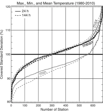
In Fig.1, the percentage of observed standard deviation which is covered by the model time series using a 24-h and 144-24-h forecast 24-horizon, respectively, is s24-hown for each station. For better readability, the stations are sorted in order of increasing percentage of covered standard deviation. The analysis is done for daily mean, maximum, and minimum temperatures, respectively. Due to the individual sorting, the three temperatures do not correspond to each other at a given location on the x-axis. It can be seen that the range of variation in mean and maximum temperature is captured well and very similar to each other, with almost all stations cov-ering at least 90% of the observed standard deviation. Interestingly, the covered standard deviation does not increase if the forecast horizon is extended to 144 h. For mean and maximum temperatures, the differences are negligible. For minimum temperature, the standard
de-Max., Min., and Mean Temperature (1980-2010)
0 100 200 300 400 500 600 Number of Station 80 90 100 110 120 Co v ered Standard De viation (%) min mean max 24 h 144 h
Fig. 1 Percentage of the observed (1980–2010) standard
devia-tion which is covered by model forecast data from 2008 to 2010. Model data of the first 24 and 144 forecast hours of each daily run are shown, respectively
viation even decreases which seems counter-intuitive. The effect is most likely caused by initial conditions and the model spin up to local conditions, which are weighted more if the forecast horizon is shorter.
About half the stations overestimate the standard deviation slightly, but mostly by less than 5%. The over-estimation of maximum temperature is 3–4% larger than for mean temperature at about 10% of all stations. The captured variation of daily minimum temperature is about 7% less than for mean and maximum values. Hence, over 90% of all stations underestimate the vari-ation of minimum temperature, indicating either a too short model time series or a problem in the prediction of minimum temperatures in the model itself.
To further investigate this, Fig.2is similar to Fig.1
but the observed standard deviation is computed only for the 3 years corresponding to the model data. About 200 more stations are considered in this analysis, as the criteria for 20 years of observations does not have to be met anymore. It can be seen that the underestimation in the variation of daily minimum temperature is the same as when compared to 30 years of observations. Hence, the problem can be attributed to the forecast model. Interestingly, there are also more stations that underestimate the variation of daily mean and maxi-mum temperatures. This could mean that, on average,
Max., Min., and Mean Temperatre (2008-2010) 0 200 400 600 800 Number of Station 60 70 80 90 100 110 120 Co v ered Standard De viation (%) mean max min
Fig. 2 Percentage of the observed (2008–2010) standard
devia-tion which is covered by model forecast data from 2008 to 2010. Model data of the first 24 h of each daily run are shown
more extreme events occurred in 2008–2010, as the model time series from this period leads to a larger overestimation of variance when compared to 30 years of observations.
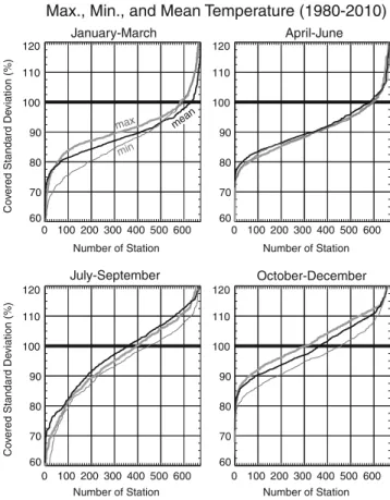
The results shown in Fig.1are very promising but could be caused by averaging over all seasons. Namely, a given station could significantly overestimate the vari-ance in summer and underestimate it in winter. Figure3
summarizes the analysis for groups of 3 months. It can be seen that the seasonal averaging has some positive effect. Interestingly, the second half of the year has more stations were the observed variance is overesti-mated by the model. Furthermore, the underestimation of the daily minimum temperature variance is only present in the cold season. It has to be mentioned again that due to the sorting of stations, no direct compar-isons between stations can be made, neither between variables nor between seasons.
3.2 Heating and cooling degree days
The representativeness of the model time series has been analyzed above, but it remains difficult to assess its value for a practical application. In the following, heating and cooling degree days are investigated as an example, as they are the basis of many practical
appli-Max., Min., and Mean Temperature (1980-2010)
0 100 200 300 400 500 600 Number of Station 60 70 80 90 100 110 120 Co v ered Standard De viation (%) 0 100 200 300 400 500 600 Number of Station 60 70 80 90 100 110 120 0 100 200 300 400 500 600 Number of Station 60 70 80 90 100 110 120 Co v ered Standard De viation (%) 0 100 200 300 400 500 600 Number of Station 60 70 80 90 100 110 120 January-March April-June July-September October-December mean
Fig. 3 Percentage of the observed 3-monthly (1980–2010)
stan-dard deviation which is covered by model forecast data from 2008 to 2010. Model data of the first 24 h of each daily run are shown
cations. Furthermore, degree days incorporate a more direct verification, namely the absolute temperatures have to be representative, not just the variance, in order to get a realistic degree-day sum.
3.2.1 Heating degree days
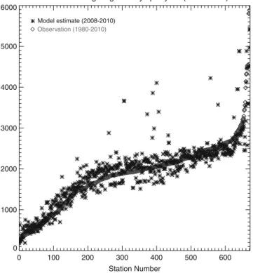
Figure4shows the mean yearly sum of heating degree days for every station. The observed values are sorted in increasing order, and the corresponding modeled values are plotted for every station, thus allowing direct comparisons. For the observed data, the yearly mean is computed from 20 to 30 years of daily observations depending on data availability of the station. For the model, the 3 years of the 24-h forecast horizon are used. It can be seen that the modeled values group nicely around the observations. The mean error over all stations is 0.07 heating degree days, which is perfect. Thus, there is no bias across all stations; but in practical applications, only some stations are of interest, and the errors will not cancel out in this way. The mean
Mean Heating Degree Days per year (1980-2010) 0 100 200 300 400 500 600 Station Number 0 1000 2000 3000 4000 5000 6000 Model estimate (2008-2010) Observation (1980-2010)
Fig. 4 Mean yearly heating degree days as observed from 1980 to
2010 and modeled with weather forecast data from 2008 to 2010
absolute and RMS error are 153 and 194 degree days, respectively.
Figure 5 shows a histogram of the absolute and relative error of the yearly mean heating degree days. The majority of stations have a relative error of less than 20% or about 250 heating degree days in absolute terms. It can be seen that the error distribution has a small negative preference, meaning that there are more stations where the forecast model overestimated
Heating Degree-Days (absolute error)
-600 -400 -200 0 200 400 600 Error (degree-days) 0 20 40 60
Stations per Bin
day1 only day 1-6
Heating Degree-Days (relative Error)
-60 -40 -20 0 20 40 60 Error (%) 0 50 100 150 day1 only day 1-6
Fig. 5 Histogram of absolute and relative error for the model
estimated climatological heating degree days. Shown are the results if the first 24 or the full 144 forecast hours for each day are used, respectively
temperature and hence underestimated the required heating. Section 3.2.3 will illustrate that a clear geo-graphical pattern of this bias exists. As mentioned in Section2.2, the model computed a 144-h forecast each day, resulting in six different forecasts for each day. Mean yearly cooling degree days as observed from 1980 to 2010 is presented in Fig.6; Figs.5and7illustrate the effect of extending the forecast horizon to 144 forecast hours. Surprisingly, the results are very similar. On one hand, the forecast skill decreases over time, leading to quite wrong forecasts. On the other hand, the larger forecast horizon captures more possible weather situ-ations and reducing the gap between 3 years of model data and 30 years of observations. However, the net effect seems to be relatively small.
3.2.2 Cooling degree days
Figure 6 presents yearly cooling degree days. Oppo-site to the heating degree days, this gives more room for error in warmer climates than in colder climates where almost no cooling is required. Across all stations, there is a small underestimation of the annual mean cooling degree days (−22). The absolute error is 88 cooling degree days, which is about half the error of the
Mean Cooling Degree Days per year (1980-2010)
0 100 200 300 400 500 600 Station Number 0 500 1000 1500 2000 2500 3000 Model estimate (2008-2010) Observation (1980-2010)
Fig. 6 Mean yearly cooling degree days as observed from 1980 to
Cooling Degree Days (absolute Error) -600 -400 -200 0 200 400 600 Error (Degree-Days) 0 20 40 60 80 100 120
Stations per Bin
day1 only day 1-6 -60 -40 -20 0 20 40 60 Error (%) 0 20 40 60 80 day1 only day 1-6 Cooling Degree Days (relative Error)
Fig. 7 Histogram of absolute and relative error for the model
estimated climatological cooling degree days. Shown are the results if the first 24 or the full 144 forecast hours for each day are used, respectively
heating degree days. This smaller error might be caused by the smaller error in daily minimum temperature during the summer, when most cooling is required, as opposite to the heating, which takes place in winter, when the error of minimum temperature is larger. The very warm and very cold climates are estimated with high accuracy, and most of the error is found for sta-tions having between 250 and 1,000 cooling degree days per year.
Figure7shows a histogram of the absolute and rela-tive error for the annual mean cooling degree days. The absolute error shows not only a narrower distribution than for heating degree days but also a negative pref-erence so that the model more often underestimates the required cooling. Even though, the absolute error for most stations is less than 150 degree days and thus better than for heating degree days, the relative error is significantly larger. This is mostly an arithmetic effect due to low degree-day totals at many stations. Again, the difference between the 24-h and 144-h forecast horizon is small. In regions where significant cooling is required, the relative error is around 5–10% for most stations which will be further analyzed next.
3.2.3 Geographical patterns
It is interesting to see if the model estimates have re-gional biases or if errors are randomly distributed over all climatic zones. Note that regional biases could be corrected with relative ease, as compared to randomly distributed biases.
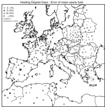
In Fig.8, the spatial distribution of the relative er-ror of yearly mean heating degree days is shown. A clear East–West difference can be observed with an underestimation in the East and an overestimation of the required heating in the West. A really homogenous
0 - 5% 5-10% 10-15% >15%
Heating Degree-Days - Error of mean yearly total
Fig. 8 Spatial distribution of the relative error of modeled mean
yearly heating degree days. Observation from 1980 to 2010 and weather forecast data from 2008 to 2010 were used
pattern exists in Poland and neighboring countries with errors below 5–10%. Equally good results are found in Denmark, Germany, the Netherlands, Belgium, and the UK; however, more outliers can be found. In France, an increase of the error towards the South can be observed. In Spain and northern Africa, no clear spatial patterns emerge, and the relative error can exceed 15%. However, heating in warm climates is relatively unimportant when compared to the amount of energy required for cooling. Hence, a good estimation of cool-ing degree days should be achieved in these climates.
Figure 9 shows the relative error of yearly mean cooling degree days. An East–West difference between overestimation and underestimation still exists but is less pronounced than for heating degree days. The warm climates of Northern Africa, Italy, Greece, Por-tugal, and Spain have a relatively homogenous pattern of small errors. In cooler climates such as the UK and Ireland, the relative error can exceed 20%. Also in Switzerland and France, errors exceeding 20% of the observed values are very frequent. However, the absolute cooling degree-day number is also low in these countries.
Using all model grid points, maps of annual mean heating and cooling degree days can be computed and are shown in Figs. 10 and 11, respectively. As these maps are based on model data, information is not lim-ited to land mass or regions with weather observations.
0 - 5% 5-10% 10-20% >20%
Cooling Degree-Days - Error of mean yearly total
Fig. 9 Spatial distribution of the relative error of modeled mean
yearly cooling degree days. Observation from 1980 to 2010 and weather forecast data from 2008 to 2010 were used
The maps should be used together with Figs.8and9to estimate the expected regional uncertainty and quality of the maps.
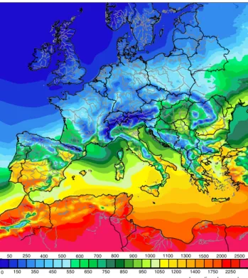
300 700 900 1100 1300 1500 1700 1900 2100 2400 2800 3300 3800 100 500 800 1000 1200 1400 1600 1800 2000 2200 2600 3000 3600 4000
mean yearly heating degree-days
Fig. 10 Mean yearly heating degree days as estimated from
numerical weather prediction data
150 350 450 550 650 750 850 950 1050 1200 1400 1750 2250 50 250 400 500 600 700 800 900 1000 1100 1300 1500 2000 2500
mean yearly cooling degree-days
0
Fig. 11 Mean yearly cooling degree days as estimated from
numerical weather prediction data
4 Discussion
The heating and cooling degree days are a common measure for the energy management of infrastruc-tures. While the climatological values of heating and cooling degree days are used for the initial planning of a building, the forecasted weather data could be used to manage the energy consumption. Müller (2011) showed that temperature forecasts with suitable post-processing provide a high accuracy, even for hourly time resolution.
The quality of estimated heating and cooling degree days is very satisfying, especially in considering local variations of temperature and errors of representative-ness between a model grid cell and an observation station. The model estimate might have a systematic regional bias as seen in Eastern Europe. However, already a coarse network of observations would show the bias and corrections to the forecast can be applied.
As shown by Müller (2011), temperature fore-casts can be significantly improved by statistical post-processing, which would also improve the estimation of heating and cooling degree days. However, as the model-derived estimates are intended to be used in locations where no observations are available, a post-processing depending on observational data is not rep-resentative or possible in practice.
5 Conclusions
An analysis of the suitability of 3 years of archived temperature forecasts as a surrogate for 30 years of real observations was carried out. For the 700 weather stations used in Central Europe, the model estimated standard deviations for daily mean and maximum tem-peratures were between 90 and 110%. The captured standard deviations for minimum temperatures were about 5% lower. A seasonal analysis reveals that this underestimation only occurs in the winter. Interest-ingly, when the observational period is shortened to the 3 years (2008–2010) of model data, the captured stan-dard deviation decreases in a way that overestimation occurs at fewer stations. This means that the model time series of 3 years is long enough to capture the stan-dard deviation of the 30-year observational period. In fact, an overestimation of about 5% exists for half the stations. Furthermore, the 2008–2010 subperiod had a larger standard deviation than the 1980–2010 period. Extending the forecast horizon of the model to 144 h yields six different forecasts for each day of the 3-year period. As the forecasts are not perfect, this adds more possible weather situations to the model data, which could be interpreted as a longer time series. However, the captured standard deviations are almost identical, regardless of the length of the forecast horizon.
An important measure used in engineering and agri-culture are degree days. Furthermore, degree days require accurate forecasts for realistic estimates and hence are a good verification tool. The comparison between modeled and observed degree days are very satisfying. Heating degree days can be estimated with a mean absolute error around 150 degree days. This corresponds to an error smaller than 20% for almost all stations and errors of only 5–15% for stations in cli-mates where heating is important. Esticli-mates for cooling degree days are even better. The mean absolute error over all stations is around 90 degree days. However, as annual totals are lower than for heating degree days, the relative error is larger and around 20–30%. But again, in climates where cooling degree days are important, the error is on the order of only 10–15%. Based on model data, which has been verified against the 30-year observational record, maps for heating and cooling degree days in Central Europe were computed. Based on the 700 verification locations, the regional uncertainty of the estimate could be quantified.
For some practical applications, model data can be used as a surrogate for long observational data records. This not only simplifies administrative difficulties of obtaining climate data but also opens the possibility to get relatively accurate estimates in places where no observations are available. It has to be noted that ap-plications focusing on extreme events could very likely not use such an approach.
Acknowledgements We would like to thank the NCDC in
Asheville, NC for providing the observational data used in this study. Furthermore, we would like to express our gratitude to the anonymous reviewers.
References
Allen JC (1976) A modified sine wave method for calculating degree days. Environ Entomol 5:388–396
Arnold CY (1974) Predicting stages of sweet corn development. J Am Soc Hortic Sci 99:501–505
van Asseldonk MAPM (2003) Insurance against weather risk: Use of heating degree-days from non-local stations for weather derivatives. Theor Appl Climatol 74:137–144 Colombo AF, Etkin D, Karney BW (1999) Climate variability
and the frequency of extreme temperature events for nine sites across Canada: implications for power usage. J Climate 12:2490–2502
Day T (2006) Degree-days: theory and application, TM, vol 41. The Chartered Institution of Building Services Engineers, London, UK.
Eto JH (1988) On using degree-days to account for the effects of weather and annual energy use in office buildings. Energy Build 12:113–127
Foster JE, Taylor PL (1975) Thermal-unit requirements for de-velopment of the Hessian Fly under controlled environ-ments. Environ Entomol 4:195–202
Janjic ZI (2003) A nonhydrostatic model based on a new ap-proach. Meteorol Atmos Phys 82:271–285
Janjic ZI, Gerrity JP, Nickovic S (2001) An alternative approach to nonhydrostatic modeling. Mon Weather Rev 129:1164– 1178
McVicker IFG (1946) The calculation and use of degree-days. J Inst Heat Vent Eng 14:252–299
Müller MD (2011) Effects of model resolution and statistical postprocessing on shelter temperature and wind forecasts. J Appl Meteor Climatol 50:1627–1636
Plett S (1992) Comparison of seasonal thermal indices for mea-surement of corn maturity in a prairie environment. Can J Plant Sci 72:1157–1162
Quayle RG, Diaz HF (1980) Heating degree-day data applied to residential heating energy consumption. J Appl Meteorol 19:241–246
Wilks DS, Wilby RL (1999) The weather generation game: a re-view of stochastic weather models. Prog Phys Geogr 23:329– 357