HAL Id: hal-00996779
https://hal.inria.fr/hal-00996779
Submitted on 26 May 2014
HAL is a multi-disciplinary open access
archive for the deposit and dissemination of
sci-entific research documents, whether they are
pub-lished or not. The documents may come from
teaching and research institutions in France or
abroad, or from public or private research centers.
L’archive ouverte pluridisciplinaire HAL, est
destinée au dépôt et à la diffusion de documents
scientifiques de niveau recherche, publiés ou non,
émanant des établissements d’enseignement et de
recherche français ou étrangers, des laboratoires
publics ou privés.
Optimizing IGP Link Weights for Energy-efficiency in a
Changing World
Joanna Moulierac, Khoa Phan
To cite this version:
Joanna Moulierac, Khoa Phan. Optimizing IGP Link Weights for Energy-efficiency in a Changing
World. [Research Report] RR-8534, INRIA. 2014, pp.21. �hal-00996779�
0249-6399 ISRN INRIA/RR--8534--FR+ENG
RESEARCH
REPORT
N° 8534
May 2014Optimizing IGP Link
Weights for
Energy-efficiency in a
Changing World
RESEARCH CENTRE
SOPHIA ANTIPOLIS – MÉDITERRANÉE
Energy-efficiency in a Changing World
Joanna Moulierac
∗ †, Truong Khoa Phan
† ∗Project-Teams COATI
Research Report n° 8534 — May 2014 — 18 pages
Abstract: Recently, saving energy for backbone networks has raised an increasing concern
for network operators. Since traffic load has a small influence on power consumption, the most common approach is to put unused links into sleep mode to save energy. To guarantee QoS, all traffic demands should be routed without violating capacity constraints. In this work, we consider to save energy with Open Shortest Path First (OSPF) protocol. From the perspective of traffic engineering, we argue that stability in routing configuration also plays an important role in QoS. In details, frequent changes in network configuration (link weights, slept and activated links) to adapt with traffic fluctuation in daily time cause network oscillation. We propose a novel optimization method of link weight so as to limit the changes in network configurations in multi-period traffic matrices. We formally define the problem and model it as Mixed Integer Linear Program (MILP). We then propose efficient heuristic algorithm that is suitable for large networks. Simulation results with real traffic traces on three different networks show that our approach achieves high energy savings and less pain for QoS (in term of less changes in network configuration).
Key-words: Robust Network Optimization, Energy-aware Routing, Green Networking, Traffic
Engineering.
∗Inria, France
Optimizing IGP Link Weights for Energy-efficiency in a
Changing World
Résumé : Depuis quelques années, les opérateurs rèseaux se sont plus particulièrement
intéressés à économiser de l’énergie dans leurs réseaux de coeur. Comme plusieurs études ont montré que la charge de trafic a une faible influence sur la consommation d’énergie des routeurs, une approche naturelle pour économiser l’énergie est de mettre en veille des liens peu utilisés. Pour garantir un certan niveau de qualité de service, toutes les requêtes doivent pouvoir être acheminées tout en respectant les contraintes de capacité de liens. Dans ce travail, nous étudions plus particulièrement cette problématique appliquée avec le protocole de routage OSPF (Open Shortest Path First). Du point de vue de l’ingénierie du trafic, nous pensons que la stabilité de configuration de routage est un paramètre important pour la qualité de service. En pratique, les changements trop fréquents de configuration de réseau (métriques de lien, liens on/off) ne sont pas souhaitables car ils peuvent causer d’importantes oscillations. Nous proposons dans ce papier une nouvelle méthode d’optimisation des métriques des liens de manière à limiter les changements de configurations réseau lorsque le trafic est dynamique (plusieurs matrices de trafic). Nous définissons formellement le problème et le modélisons comme un programme linéaire mixte en nombre Entier. Nous proposons ensuite une heuristique efficace qui convient pour les réseaux de plus grande taille. Les résultats de simulation avec des matrices de trafic réèlles sur trois réseaux différents montrent que notre approche permet d’obtenir des économies d’énergie intéressantes tout en préservant un certain niveau de qualité de service (car moins de changements de configurations réseau).
Mots-clés : Robust Network Optimization, Energy-aware Routing, Green Networking, Traffic
1
Introduction
Recent studies have shown that ICT is responsible for 2% to 10% of the worldwide power con-sumption [1, 2]. For example, the Global e-Sustainability Initiative estimated an overall network energy requirement for European telecommunication is around 35.8 TWh in 2020 [3]. As estima-tion, energy consumption of backbone networks can increase to 40% of the total network power requirements by 2017 [4]. Therefore, saving energy for backbone networks have become an active networking research area. While the traffic load has a marginal influence, the power consumption is mainly due to active elements on IP routers such as ports, line cards, base chassis, etc. [5]. Based on this observation, the energy-aware routing (EAR) approach aims at minimizing the number of used links while all the traffic demands are routed without any overloaded links [2, 6]. In fact, turning off entire routers can earn significant energy savings. However, it is difficult from a practical point of view as it takes time for turning on/off and also reduces life cycle of devices. Therefore, as in many existing works [7, 8], we assume to turn off (or put into sleep mode) only links to save energy.
Although green networking has been attracting a growing attention during the last years (see the surveys [9, 10]), we found a limited number of recent works that have been devoted to energy-aware traffic engineering [11, 12, 13, 14]. These works consider the most widely used Internal Gateway Protocol (IGP) in IP networks, namely the Open Shortest Path First (OSPF) protocol. This link state approach performs a local calculation of shortest paths based on a set of link weights. This avoids optimizing routing on a per-flow basis (like MPLS-TE) which can be complex when a large number of traffic demands is considered. In summary, these works try to find an OSPF weight setting that routes the traffic in a shortest path manner while it minimizes the number of active routers/links. Inactive network elements will be put into sleep mode to save energy.
To deal with traffic variation, daily time periods are characterized by different traffic levels (e.g. morning, afternoon and night) and in each period, a single traffic matrix is assumed to be accurately collected. As traffic matrices are considered independently, different sets of link weights are assigned for each traffic matrix. As assumed in existing works [11, 12, 13], as long as the network capacity is sufficient for handling all traffic demands, energy can be saved without causing service deteriorations to end users. However, from the view point of traffic engineering, the routing protocol can affect a lot on QoS. For instance, as explained in [15], we should avoid link weight changes as much as possible. First, we note that even a single weight change is disruptive for a network. The weight change has to be flooded in the network via control messages. The routers then recompute the shortest paths and update their routing tables. This may take seconds before all routers agree on the new shortest paths. Meanwhile, in this transient time, packets may arrive out of order, degrading the perceived QoS for end-user. We refer the reader to [16] for a detailed analysis of the stability issues in OSPF. Obviously, the more weight changes we try to flood simultaneously, the more chaos we introduce in the network. Therefore, we argue that it is necessary to take into account the stability of weight setting for the energy-aware traffic engineering problem. In summary, we make the following contributions: • We formally define and formulate the stable OSPF weight setting problem for multi-periods traffic matrices using MILP. In addition, we present a Γ-robust formulation so that even a single weight setting can fit for a range of traffic variation.
• We propose heuristic algorithms that are effective for large networks.
• Using real-life data traffic traces, we show energy savings achieved by our approaches. Moreover, our simulations show that the stable weight setting methods outperform existing approaches in term of less network reconfigurations in daily traffic variation.
4 Moulierac & Phan
The rest of this paper is structured as follows. We summarize related works in Section 2. We present the MILP and heuristic algorithms in Section 3 for optimizing OSPF weight setting. Then, our approaches to deal with traffic variation are introduced in Section 4. Simulation results are presented in Section 5. Finally, we conclude the work in Section 6.
2
Related Work
2.1
Energy-aware Routing (EAR)
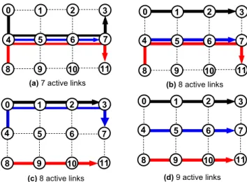
(a) 7 active links
0 10 5 1 2 3 11 6 8 9 0 10 5 1 2 3 4 11 6 7 8 9 10 5 1 2 4 11 6 7 8 9 (b) 8 active links (c) 8 active links 0 10 5 1 2 3 4 11 6 7 8 9 (d) 9 active links 4 7 0 3
Figure 1: Example of EAR and Γ-Robust network
As an example of EAR, we consider a network topology as a grid 3 × 4 (Fig. 1). Each link of the network has capacity 4 Gbps. There are three traffic demands: (0, 3), (4, 7) and (8, 11), all with volume 1 Gbps. The shortest path routing, as shown in Fig. 1d, uses 9 active links whereas the remaining 8 links can be put into sleep mode. However, since there are enough capacity to aggregate the three traffic demands as in Fig. 1a, EAR solution allows 10 links to sleep, thus energy consumption is further decreased. The problem of minimizing the number of active links under capacity constraints can be precisely formulated using Mixed Integer Linear Programming (MILP). However, this problem is known to be NP-Hard [17], and currently exact solutions can only be found for small networks. Thus, many heuristic algorithms have been proposed to find admissible solutions for large networks [17, 2].
From the view point of traffic engineering, MPLS-TE can be used to deploy energy-aware routing in a network. However, as we have argued, MPLS-TE is complex for large network with many traffic demands since we need to do configuration on a per-flow basis. Recently, a few works have been devoted to energy-aware traffic engineering using OSPF protocol [11, 12, 13]. These works try to optimize link weight setting so that the shortest path routing uses a minimum number of active links. An example on OSPF weight setting for energy-aware routing will be shown in Section 3.
Since traffic varies over time, these works [11, 12, 13] have to apply a large number of config-urations in daily time, one for each traffic matrix. This causes serious oscillation for a network as mentioned in Section 1. To the best of our knowledge, the closest papers to our work are from [7, 11, 18, 12, 13]. In [7], a limited number of configurations are applied to a network during
daily traffic variation. Meanwhile in [18], the authors have proposed a robust network model to deal with traffic variation. However, these work are not dedicated for OSPF protocol, and stabilizing link weight setting is not mentioned. In [11, 12, 13], the authors try to optimize the OSPF weight setting for each single traffic matrix. However, it may cause network oscillation as many network reconfigurations occur during multi-period traffic matrices. In our work, we focus on the stability of link weight setting in OSPF/ECMP protocol. Along with the exact model (MILP), we also propose efficient heuristic algorithms for large networks.
2.2
Γ-Robust Network Design
Over the past years, robust optimization has been established as a special branch of mathematical optimization allowing to handle uncertain data [19]. A specialization of robust optimization, which is particularly attractive by its computational tractability, is the so-called Γ-robustness concept introduced by Bertsimas and Sim [20]. Based on an observation that in real traffic traces, at a given time, only few of the demands are simultaneously at their peaks. Γ-robust network design allows to choose an integer parameter Γ ≥ 0 so that at most Γ traffic demands can be at their peak values simultaneously. Note that, the model only limits a number of traffic demands (but not exactly which ones) that can be at their peaks at the same time. Therefore, from a practical perspective, by varying the parameter Γ, different solutions can be obtained with different levels of robustness. This concept has already been applied to several network optimization problems [21, 18, 22].
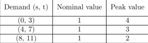
To better explain, we consider an example in Fig. 1. Again, we use a grid 3 × 4, each link has a capacity 4 Gbps (Fig. 1). There are 3 traffic demands, each has a nominal and peak values (in Gbps) as shown in Table 1.
Table 1: Traffic demand variation
Demand (s, t) Nominal value Peak value
(0, 3) 1 4
(4, 7) 1 3
(8, 11) 1 2
Assume that we choose Γ = 2, this means in the network, it is possible to have zero, one or two traffic demands that are at their peaks simultaneously. This forms a combination of seven possibilities (cases) as shown in Table 2: Q is a set containing demands that can be at their peak values.
It is easy to see that in Case 1, all traffic demands are at nominal values, hence as EAR, Fig. 1a is the best solution with only 7 active links. In Case 2, when (0, 3) is at peak (4 Gbps), solutions in Fig. 1b and Fig. 1d are feasible. However, Fig. 1b is the best solution since only 8 active links are used. Similarly, in Case 7, solutions in Fig. 1c and Fig. 1d are feasible and Fig. 1c is the best one. In summary, Table 2 shows the complete possibilities of traffic variation and the corresponding best solution when Γ = 2. However, since we just limit the number demands (but not any specific demands) to be deviated, a feasible solution should be the one that satisfies all the seven cases. Therefore, Fig. 1d is the only feasible solution for Γ = 2. It is also easy to check that, if we limit Γ = 1 (less robust), Fig. 1b is the best solution. From these examples, we can see that, depending on the desired robustness of a network, a single routing solution can be feasible for many traffic matrices. This is why we propose in Section 4.2 a robust model that can find a single network configuration for a range of traffic variation.
6 Moulierac & Phan
Table 2: Example of robustness: Γ = 2
Case Q Best solution Link load luv(Gbps)
1 {} Fig. 1a l0,4= l7,3= 1, l4,5,6,7= 3, (7 links) l8,4= l7,11= 1 2 {(0, 3)} Fig. 1b l0,1,2,3= 4, l4,5,6,7= 2, (8 links) l8,4= l7,11= 1 3 {(4, 7)} Fig. 1b or 1c l0,1,2,3= 1, l4,5,6,7= 4, (8 links) l8,4= l7,11= 1 (Fig. 1b) 4 {(8, 11)} Fig. 1a l0,4= l7,3= 1, l4,5,6,7= 4, (7 links) l8,4= l7,11= 2 5 {(0, 3), (4, 7)} Fig. 1b l0,1,2,3= 4, l4,5,6,7= 4, (8 links) l8,4= l7,11= 1 6 {(0, 3), (8, 11)} Fig. 1b l0,1,2,3= 4, l4,5,6,7= 3, (8 links) l8,4= l7,11= 2 7 {(4, 7), (8, 11)} Fig. 1c l0,1,2,3= 4, l4,0= l3,7= 3, (8 links) l8,9,10,11= 2
3
Optimizing weight setting for EAR
EAR routing can be applied to a network by setting an appropriate link weight setting. By assigning a high value of weight to a set of links, no traffic passes through them, thus we can put these links into sleep mode to save energy.
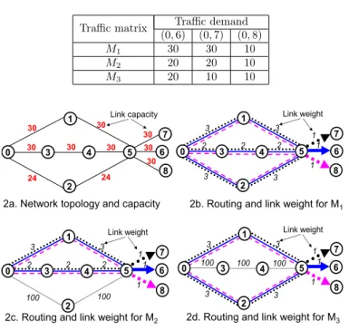
Table 3: Traffic matrices for OSPF/ECMP
Traffic matrix Traffic demand (0, 6) (0, 7) (0, 8) M1 30 30 10 M2 20 20 10 M3 20 10 10 2 0 1 8 7 6 5 4 3 30 30 30 30 30 24 24 30 30 30 Link capacity
2a. Network topology and capacity
2 0 1 5 4 3 3 2 Link weight 3 3 3 2 2 1 1 1 8 7 6 2 0 1 5 4 3 3 2 Link weight 3 100 100 2 2 1 1 1 8 7 6 2 0 1 5 4 3 3 100 Link weight 3 3 3 100 100 1 1 1 8 7 6
2c. Routing and link weight for M2 2d. Routing and link weight for M3
2b. Routing and link weight for M1
Figure 2: Example of OSPF/ECMP for EAR
To better explain, we consider an example of a network topology with capacity on links as shown in Fig. 2a. There are 3 traffic demands and we collect their values at 3 different periods,
leading to 3 traffic matrices M1, M2 and M3 (Table 3). The routing solutions in Fig. 2 follow OSPF/ECMP (Equal-cost multi-path) policy: when there are multiple shortest paths, traffic is equally splitted among these paths. As shown in Fig. 2b, the three traffic demands are splitted into 3 different paths from 0 to 5, each path carries (30 + 30 + 10)/3 = 70/3 < 24. So, this routing is feasible but zero link can sleep. When traffic decreases, we can have better solutions.
For example, 2 and 3 links are put in sleep mode for M2(Fig. 2c) and M3(Fig. 2d), respectively.
The problem of optimizing OSPF weight setting is known to be NP-hard [23], exact formulation and heuristic algorithm have been proposed.
3.1
Mixed Integer Linear Program
Based on [11] and to fit with our robust model (Section 4.B), we reformulate the OSPF weight setting problem for energy-aware routing as follows:
min ∑ (u,v)∈E xuv (1) s.t. ∑ v∈N (u) ( fst vu− f st uv ) = −1 if u = s, 1 if u = t, 0 else ∀u ∈ V, (s, t) ∈ D (2) ∑ (s,t)∈D Dst(fst uv+ f st vu) ≤ µCuvxuv ∀(u, v) ∈ E (3) 0 ≤ zust− f st uv≤ 1 − k t uv ∀(s, t) ∈ D; (u, v) ∈ E (4) fuvst − k t uv≤ 0 ∀(s, t) ∈ D; (u, v) ∈ E (5) 1 − ktuv≤ r t v+ wuv− rtu≤ (1 − k t uv)M ∀t ∈ Dt; (u, v) ∈ E (6) ktuv− xuv≤ 0 ∀t ∈ Dt; (u, v) ∈ E (7) wuv≥ (1 − xuv)wmax ∀(u, v) ∈ E (8) xuv+ wuv≤ wmax ∀(u, v) ∈ E (9) 1 ≤ wuv≤ wmax ∀(u, v) ∈ E (10) xuv, kuvt ∈ {0, 1}; f st uv, z st u ∈ [0, 1]; r t u≥ 0 (11)
where wmax is the maximum value of a link weight. M is a large enough constant, it can
be set M = 2wmax. Dt is a set containing all destination nodes. The objective function (1)
minimizes the power consumption of the network represented by the number of active links. Constraints (2) establish the classical flow conservation constraints. We consider an undirected link capacity model [24] in which the capacity of a link is shared between the traffic in both directions. Constraints (3) limit the available capacity of a link (where µ denotes the maximum
link utilization). The binary variable kt
uv = 1 if and only if the link (u, v) belongs to one of the
shortest paths from node u to node t. Constraints (4) are for ECMP routing. It makes sure that if kt
uv= 1 then the flow fvust destined to node t is equal to zut, which is the common value of the
flow assigned to all links outgoing from u and belonging to one of the shortest paths from u to t.
Constraints (5) force fst
uv= 0 for all links (u, v) that do not belong to a shortest path to node t.
The variable rt
urepresents the length of the shortest path from u to t. Constraints (6) compute
weight of the link (u, v) if it belongs to the shortest path from u to t. Constraints (7) force link
(u, v) to be on if it belongs to the shortest path from u to t. Note that, we do not force xuv= 0
when kt
uv= 0 because if (u, v) belongs another shortest path to t1 (in this case kuvt1 = 1 and xuv
should be equal to 1). The constraints (8)-(10) guarantee that if a link weight is equal to wmax,
8 Moulierac & Phan
3.2
Heuristic Algorithm
Finding optimal OSPF weight setting that deals with energy savings and/or traffic engineering issues is very challenging. We found in literature many work trying to solve this problem using heuristic approaches. For example, the authors in [23, 11] have proposed to use local search by iteratively modifying the OSPF weights so as to achieve the objective. Francois et al. [12] have used genetic algorithms to find the link weights for the joint-optimization of load-balancing and energy efficiency. As the traffic matrices are considered independently, these methods find different sets of link weights in the optimization process for each traffic matrix. Thus, the link weight settings can be different for each traffic matrix, thus we call these methods as freely changed weight setting.
Our goal in this work is not to compare with these heuristics to see which method can achieve a better energy efficient solution. In this work, we focus on a rather different objective. As presented in Section I, we should avoid weight changes as many as possible. For this reason, we propose in this paper methods to stabilize the OSPF weight setting (called stable weight setting), so as to reduce the slide effects when deploying energy-aware routing for a backbone network. To give an idea of energy savings, we have implemented a simple freely changed weight
setting algorithm (in Section 4.1.3) to compare with the stable weight setting approach.
4
How to deal with OSPF weight setting in a changing
world?
4.1
Stable Weight Setting
In this approach, multi-period traffic matrices are used to capture the daily traffic pattern. However, these traffic matrices are not considered independently. The idea is that, when changing from a high to a lower traffic matrix (traffic load is reducing), we only consider to sleep unused links. In addition, the weight setting of remaining links are unchanged. The reason is to limit changes in routing configuration and reduce network oscillations that affect QoS. As we add restriction, stable weight setting has less potential in savings energy than the freely changed
weight setting approach. For instance, as the example in Fig. 2, when traffic changes from M2
to M3, the stable weight setting can not have solution like Fig. 2d. It is because it needs both
to turn on and off links which causes serious chaos when shifting between multi-period traffic matrices. However, as we show in Section 5, using real traffic traces, the energy savings gap between stable weight and freely changed weight methods is quite small.
Since we try to stabilize the weight setting based on the previously used one, a question is how to find an initial weight setting that will be used for all the matrices of the multi-period traffic matrices. In fact, there are many ways to set link weights in practice. For instance, Cisco uses the inverse of link capacity [25]; or more complicated load-balancing traffic engineering methods can be found in [15, 11, 12]. Actually, the initial set of weight has an impact on the energy savings in daily time. We can use the freely changed weight method to find a good configuration for a traffic matrix. However, this configuration may not be good for subsequent traffic matrices and how to find a good starter for the whole day traffic variation is beyond the scope of this paper. In this work, the network operators are free to choose their own weight setting. Anytime they would like to start energy savings mode, the stable algorithm can be applied directly using the current weight setting configuration as the initial one. We propose an optimization formulation and heuristic algorithms for the stable weight setting method as follows:
4.1.1 Stable Weight MILP
The inputs are network topology G = (V, E), traffic matrix D and a set of current link weights W . The output is a routing solution that minimizes number of active links so that it satisfies constraints (2) - (11). Meanwhile, as the weight setting W should not be modified, following constraints should be added to the model (1) - (11):
wuv− wuv∗ ≥ (1 − xuv)(wmax− w∗uv) ∀(u, v) ∈ E (12)
wuv∗ − wuv ≥ (xuv− 1)wmax ∀(u, v) ∈ E (13)
We note w∗
uv as the current weight of the link (u, v). Constraints (12) - (13) are used to force
the new link weight wuv to be equal to w∗uv if the link (u, v) is still used in the new routing
solution. Otherwise, wuv is set to wmax and the link (u, v) is put into sleep mode.
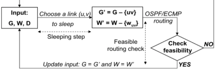
4.1.2 Stable Weight Heuristic
The stable weight setting problem is also very challenging for large networks. We propose in this section heuristic algorithms that can find feasible solution in an acceptable time. In brief, the heuristic algorithm includes sleeping step and feasible routing check step (Fig. 3).
Check feasibility Input:
G, W, D
Choose a link (u,v) to sleep G’ = G – {uv} W’ = W – {wuv} OSPF/ECMP routing NO
Mark the link (u, v) as already checked link
YES
Update input: G = G’ and W = W’
Sleeping step
Feasible routing check
Figure 3: Heuristic diagram
There are many criteria to choose a link (u, v) to sleep (see in [11, 2]). In this paper, we propose to choose the min load link to sleep since this approach has been successfully applied in literature [11, 17, 8, 2]. After the sleeping step, the feasible routing check step has inputs which
are a subgraph G′, a subset of link weights W′ and the same traffic matrix D. We perform
OSPF/ECMP routing for D on G′ and check if some links are overloaded. If yes, the routing is
not feasible, we mark the slept link as checked and go back to the sleeping step to find another link to make sleeping (the checked links will not be chosen). If the routing is feasible, we update the inputs and go back to the sleeping step to continue. This procedure is repeated until all links on the network are checked.
To deal with multi-period traffic matrices, we first sort the traffic matrices in non-increasing
order of traffic load, that is from Dn to D1. Then, we run the MILP or heuristic algorithm for
Dnto find a feasible network configuration (link weight setting, set of links to sleep). Given this
configuration as the inputs, we find new feasible configuration for Dn−1in which we consider only
to sleep links and the remaining links keep the same weight setting. This process is repeated
until we reach D1. Following the traffic variation of daily time, from a low to higher traffic
matrices (e.g. Di to Di+1), we simply apply the configuration that has been found (from Di+1
to Di). In this scenario, only slept links are woken up and the remaining links keep the same
10 Moulierac & Phan
4.1.3 Freely Changed Weight Heuristic
In order to compare the energy savings of the stable weight heuristic, we implemented a simple
freely changed weight heuristic algorithm. Using the same diagram as in Fig. 3, at the feasible
routing check step, we follow the idea of local search used in [23]. If the routing is infeasible,
instead of marking the link as “checked”, we continue the local search to increase weights for overloaded links (to direct traffic to other links) and repeat the feasible routing check step. The number of loops in the local search can be defined depending on how much time we need the heuristic to stop. In general, the longer the computation time is, the better the solution we get.
4.2
Γ-Robust Approach: One Network Configuration for All
We propose in this sub-section a method to find a single nework configuration with a set of active links and weight setting that is feasible for all the considered traffic matrices.
4.2.1 Robust MILP
Assume that each traffic demand has a nominal Dst and a deviated value bDst so as the peak
value is (Dst+ bDst). Given a parameter 0 ≤ Γ ≤ |D|, the robust model tries to find a feasible
routing at minimal energy costs, while the link capacity constraints are satisfied if at most Γ
traffic pairs simultaneously deviate from their nominal values Dst. Note that Γ = |D| amounts
to worst-case optimization where all demands are at peak values. The straightforward robust capacity constraint for a given Γ and an edge e ∈ E is:
∑ (s,t)∈D Dstfst e + max Q⊆D |Q|≤Γ { ∑ (s,t)∈Q b Dstfst e } ≤ µCexe ∀e ∈ E (14) where fst
e = fuvst+ fvust; Q is a subset containing demands that can be at peaks at the same time.
The constraints (14) is non-linear since it contains the max notation. A trivial way to make it linear is to explicitly write down all the possibilities of the constraints, that is:
∑ (s,t)∈D Dstfest+ ∑ (s,t)∈Qi b Dstfest≤ µCexe ∀Qi⊆ D; |Qi| ≤ Γ; e ∈ E (14′)
Obviously, the constraints (14′) is a combination of all possibilities of a subset Q
i which has
the size |Qi| ≤ Γ. Therefore, it is impossible to put all the constraints into the MILP model at
one time when the set of demand D is large. To overcome this problem, we apply the method Γ-robustness (introduced by Bertsimas and Sim [20]). The main idea of this method is to use LP duality to make a compact formulation, so that it is possible to solve the MILP. We present step-by-step the procedure to form the compact formulation as follows.
Assume that we know the value of fst
e (then they are constants), the maximum part of (14)
can be computed by the following ILP:
β(f, Γ) := max ∑ (s,t)∈D b Dstfst e z st e (15) s.t. ∑ (s,t)∈D zste ≤ Γ [πe] (16) zst e ∈ {0, 1} [ρste] (17)
where the primal binary variables zst
e denote whether or not fest is part of the subset Q ⊆ D.
As proposed by Bertsimas and Sim, we employ LP duality with the dual variables πe and ρste
corresponds to the constraint ∑(s,t)∈Dzst
e ≤ Γ and z
st
e ≤ 1, respectively. The LP duality for
β(g, Γ) is as follows: β(g, Γ) := min(Γπe+ ∑ (s,t)∈D ρst e ) (18) s.t. πe+ ρste ≥ bD st fest ∀(s, t) ∈ D (19) ρst e, πe≥ 0 ∀(s, t) ∈ D (20)
Since the constraints (18)–(20) are linear. A compact reformulation can be obtained by em-bedding them into (1)–(13). As a result, the robust stable weight setting can be compactly formulated as (1)–(2), (4)–(13) and replace (3) by:
∑ (s,t)∈D (Dstfest+ ρ st e) + Γπe≤ µxeCe ∀e ∈ E (21) πe+ ρste ≥ bD st fest ∀(s, t) ∈ D; ∀e ∈ E (22) ρste, πe≥ 0 ∀(s, t) ∈ D; ∀e ∈ E (23)
4.2.2 Robust Heuristic Algorithm
The main idea of the heuristic algorithm is similar to the diagram in Fig. 3. However, is is difficult to check routing feasibility since we do not know explicitly which traffic demands are at peak values. To deal with this problem, we use the ILP constraints (21)–(23) for the feasible routing
check step as they represent the robust capacity constraints. In details, consider a simplified
MILP of the robust weight setting in which we only keep constraints (11) (remove variables kt
uv, zst
u, rtu), and (21)–(23) with xe∈ {0, 1} and fest ∈ [0, 1] ∀(s, t) ∈ D; ∀e ∈ E. The OSPF/ECMP
routing on G′ with a set of link weight W′ implicitly satisfies the flow conservation constraint.
In addition, we have in hand a set of link weight W′, therefore all the constraints (2) – (10) are
not needed in the simplified ILP. When performing OSPF/ECMP routing for the subgraph G′
(after the sleeping step), we can get all the values of fst
e and xe(xe= 0 if fest = 0 ∀(s, t) ∈ D,
otherwise xe = 1). Given them as the inputs, the variables xe and fest in the simplified MILP
are now fixed, only ρst
e and πeremain variables. Since the simplified MILP is used only to verify
routing solution, we ignore the objective function and simply set it to min 0. To check routing
feasibility, we run the simplified MILP with inputs: G′, D, Γ, fst
e and xe, if a feasible solution is
returned, it means that the routing solution satisfies the robust capacity constraints. Then, we go back to the sleeping step and continue the algorithm as in Fig. 3.
5
Computational Evaluation
We solved the MILP models with IBM CPLEX 12.4 solver [26]. All computations were carried out on a 2.7 Ghz Intel Core i7 with 8 GB RAM. We consider real-life traffic traces collected from the SNDlib [27]: the U.S. Internet2 Network (Abilene) (|V | = 12, |E| = 15, |D| = 130), the Geant network (|V | = 22, |E| = 36, |D| = 387) and the Germany50 (|V | = 50, |E| = 88, |D| = 1595).
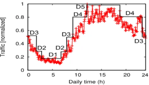
In our test instances, five traffic matrices (D1 − D5) are used to represent daily traffic pattern (Fig. 4). From the SNDlib, we collect the mean and max traffic matrices (all traffic demands are at their mean and maximum values). Since traffic load is low, we use the mean traffic matrix as D1. To achieve a network with high link utilization, we scale the max traffic matrix with a factor of 1.3, 1.5, 1.8 and 2.0, and they form D2 − D5, respectively. As a result, we represent D5 as the worst case scenario of highest traffic load. It is noted that, in realistic, even at peak
12 Moulierac & Phan 0 0.2 0.4 0.6 0.8 1 0 5 10 15 20 Traffic [normalized] Daily time (h) 24 D1 D2 D3 D2 D4 D4 D5 D3 D3
Figure 4: Daily traffic
hour, not all the traffic demands are at their maximum values as the case D5. In all test cases, as an approach of traffic engineering, we use a local search heuristic to find a set of link weights that minimize the maximum link load [23] for the traffic matrix D5. This weight setting is used as the initial one in the stable weight approaches.
5.1
Computation time
Table 4: Abilene network - optimal solutions Execution time (s)
D1 D2 D3 D4 D5
Stable weight MILP ≤ 5 ≤ 5 ≤ 5 ≤ 5 ≤ 5
Robust MILP 90
Freely changed weight MILP 95 874 100 12900 20700
Table 5: Geant network - heuristic solutions
Execution time (s)
D1 D2 D3 D4 D5
Stable weight 139 140 160 182 256
Robust stable weight 283
Freely changed weight 62 157 1596 2115 3600
Table 6: Germany network - heuristic solutions Execution time (s)
D1 D2 D3 D4 D5
Stable weight 468 1586 1787 2108 3108
Robust stable weight 3090
Freely changed weight 1739 3600 3600 3600 3600
For Abilene network, we can find optimal solution using the MILP for the three methods (stable, robust and freely changed weight). For larger network (e.g. Geant, Germany50), it is not possible to find even a feasible solution within 2 hours using the MILP, thus only the heuristic algorithms are used to find solutions for these large networks. The execution time of the freely changed weight heuristic is limited to one hour by varying the number of loops in the local search. For the robust stable weight, we run with different values of Γ and get an average running time.
It is clear that the stable weight and robust methods win a lot in running time. This is because these methods are based on an initial weight setting and we limit the change. Note that, we also
use an initial weight setting for the robust case to limit network reconfiguration when changing from the normal (currently used) mode to the energy-aware mode. Thus, solution search space is small and optimal solutions can be found quite fast. Similar observation can be found for the heuristic approaches (Tables 5 and 6): the stable weight and robust methods take less than 1 hour for all test cases, meanwhile the execution time of the freely changed weight reaches the time limit set to 1 hour.
0 1 1 2 3 4 5 6 7 8 # links ON # links OFF N u m b e r
Changing of traffic matrices in daily time
D3 → D2 D2 → D1 D1 → D2 D2 → D3 D3 → D4 D4 → D5 D5 → D4 D4 → D3 0 1 2 3 4 5 6 1 2 3 4 5 6 7 8 # links ON # links OFF # weight changes N u m b e r
Changing of traffic matrices in daily time
D1 → D2 D2 → D3 D3 → D4D4 → D5 D5 → D4 D4 → D3 D2 → D1 D3 → D2 0 1 2 3 4 5 1 2 3 4 5 6 7 8 # links ON # links OFF N u m b e r
Changing of traffic matrices in daily time
D3 → D2D2 → D1 D1 → D2D2 → D3D3 → D4D4 → D5D5 → D4 D4 → D3 0 5 10 15 20 25 30 1 2 3 4 5 6 7 8 # links ON # links OFF # weight changes N um be r
Changing of traffic matrices in daily time
D3 → D2D2 → D1D1 → D2D2 → D3D3 → D4D4 → D5D5 → D4D4 → D3 0 4 8 12 1 2 3 4 5 6 7 8 # links ON # links OFF N u m b e r
Changing of traffic matrices in daily time
D3 → D2D2 → D1 D1 → D2D2 → D3 D3 → D4 D4 → D5 D5 → D4 D4 → D3 0 10 20 30 40 50 60 70 1 2 3 4 5 6 7 8 # links ON # links OFF # weight changes N um be r
Changing of traffic matrices in daily time
D3 → D2 D2 → D1D1 → D2D2 → D3D3 → D4D4 → D5D5 → D4 D4 → D3
(a) Abilene: freely changed weight (b) Abilene: stable weight
(c) Geant: freely changed weight (d) Geant: stable weight
(f) Germany: stable weight (e) Germany: freely changed weight
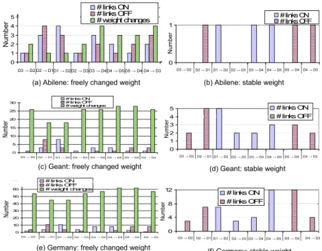
Figure 5: Changes in freely changed weight vs. stable weight methods
5.2
Stability of routing solutions
Fig. 5 shows changes in routing when shifting between periods of traffic during daily time. For the three tested networks, the stable weight approach always outperforms the freely changed weight. The former approach only allows to sleep links (resp. only wake up links) when changing from a high traffic matrix to a lower one (resp. from a low to a higher traffic matrix). However, for freely changed weight, there is no restriction, link can be turned on and off and also the weight setting of remaining links can be changed. For instance, in Abilene network, from D3 to D2, even the energy savings (and the number of active links) is unchanged, the solution allows one link to turn off, one link to turn on and two active links change their weights. Similar observation can be found for Geant and Germany networks (Fig. 5c - Fig. 5f). The larger the network we consider, the more chaos we introduce as more changes happen between multi-period traffic matrices.
14 Moulierac & Phan 0 10 20 30 1 2 3 4 5 6 7 8 9
Freely changed weight Stable weight E n e rg y sa vi n g s (% )
Traffic matrices in daily time
D3 D2 D1 D2 D3 D4 D5 D4 D3
(a) Abilene network
0 10 20 30 40 50 1 2 3 4 5 6 7 8 9
Freely changed weight Stable weight E n e r g y sa vi n g s ( % )
Traffic matrices in daily time
D3 D2 D1 D2 D3 D4 D5 D4 D3 (b) Geant network 0 10 20 30 40 50 1 2 3 4 5 6 7 8 9
Freely changed weight Stable weight E n e r g y sa vi n g s ( % )
Traffic matrices in daily time
D3 D2 D1 D2 D3 D4 D5 D4 D3
(c) Germany network
Figure 6: Energy savings in multi-period traffic matrices
5.3
Energy savings in daily time
5.3.1 Stable weight vs. freely changed weight
Follow the curve of daily traffic, we show energy savings of the three networks in Fig. 6. It is clear that energy savings is high when traffic load is low since more links can be put into sleep mode to save energy. To compare between stable weight and freely changed weight approaches, the latter one can save more energy because it is flexible to change the weight setting. This can be observed in D3, D4, D5 in Fig. 6b and D3, D5 in Fig. 6c. Abilene network is small and only a few links (from 1 to 4 links) can sleep, thus the solutions between the two methods are similar. It is noted that, in D4 (Fig. 6c), stable weight method even has better result. It is because we limit the number of loops so that the heuristic algorithm is finished after one hour. Thus, it is possible for the freely changed weight heuristic to stop before finding a better solution than the stable weight approach. It can happen when the network is large, the algorithm needs to do several loops to find a good solution.
5.3.2 Robust vs. stable weight approaches
0 5 10 15 20 25 30 35 40 45 0 5 10 15 20 energy savings (%) daily time (h) a Robust 24 Г = 0% Г = 1% Г = 2 → 3% Г = 4% Г = 8 → 100% Г = 5 → 7% Stable weight 0 5 10 15 20 25 30 0 5 10 15 20 energy savings (%) daily time (h) a Г = 0 → 7% Г = 8 → 9% Г = 10 → 13% Г = 14 → 100% Robust 24 Stable weight 0 5 10 15 20 25 30 35 40 45 0 5 10 15 20 energy savings (%) daily time (h) a Г = 0% Г = 1% Г = 2% Г = 3% Г = 4 → 6% Г = 7 → 100% Robust 24 Stable weight
(a) Abilene network (b) Geant network (c) Germany network
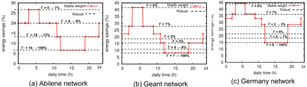
Figure 7: Robust weight vs. stable weight
Fig. 7 shows energy savings of the stable weight setting vs. the Γ−robustness (with different value of Γ) in daily time traffic variation. Simulation results confirm that the higher Γ is, the more robust, but the less power savings the solution is. Note that, when Γ = 100%, the robust model becomes the worst case of the deterministic - the case with D5 (all traffic demands are at their peak values). In all the three networks, the solutions do not change when Γ is large enough (e.g. Γ = 14% for Abilene network). It is because in real traffic, only a small fraction of the demands dominates the others in volume. Hence, when the values of Γ covers all of these
dominating demands, increasing Γ does not affect the routing solution and the percentage of energy savings remains the same. To give a visualized comparison, we also draw energy savings of the stable weight method in daily time. For instance, from Fig. 7a, if Γ = 9%, it is possible to have only one weight setting that gives feasible routing if at most 9% of traffic demands are at their peaks simultaneously. Moreover, this single weight setting allows to save a same amount of energy as when we apply the stable weight method for D2 or D3 matrices. Similar observations can be found for Geant (Fig. 7b) and Germany network (Fig. 7c). However, Geant and Germany networks are more sensitive with traffic variation, significant energy savings is found only with small Γ.
(a) Abilene network (b) Geant network (c) Germany network
0 20 40 60 80 100 0 20 40 60 80 100 Fraction of links (%) Link load (%) Freely changed weight
Stable weight 0 20 40 60 80 100 0 20 40 60 80 100 Fraction of links (%) Link load (%) Optimal freely changed weight
Optimal stable weight
0 20 40 60 80 100 0 20 40 60 80 100 Fraction of links (%) Link load (%) Freely changed weight
Stable weight
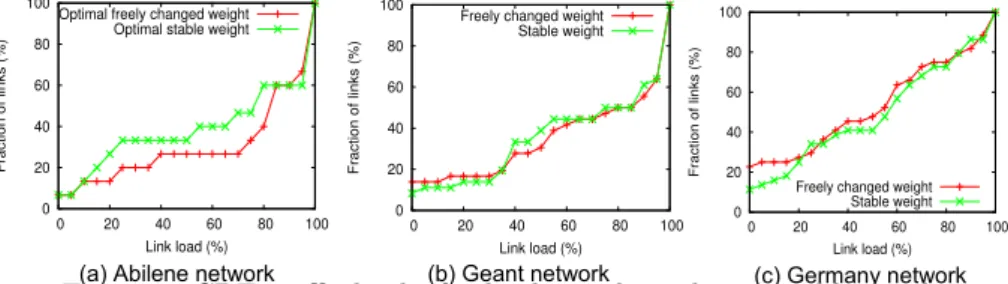
Figure 8: CDF traffic load - freely changed weight vs. stable weight
0 50 100 150 200 0 5 10 15 20 Link utilization (%) Daily time (h) Gamma = 1% - MLU (%) Gamma = 2% - MLU (%) Gamma = 100% - MLU (%) 0 50 100 150 200 0 5 10 15 20 Link utilization (%) Daily time (h) Gamma = 7% - MLU (%) Gamma = 13% - MLU (%) Gamma = 100% - MLU (%) 0 50 100 150 200 0 5 10 15 20 Link utilization (%) Daily time (h) Gamma = 1% - MLU (%) Gamma = 6% - MLU (%) Gamma = 100% - MLU (%)
(a) Abilene network (b) Geant network (c) Germany network
Figure 9: Maximum link utilization (MLU) of robust solution in daily traffic
5.4
Traffic load
5.4.1 Stable weight vs. freely changed weight
In the simulation, we set the maximum link utilization µ = 100%. Intuitively, EAR would affect the utilization of links as fewer links are used to carry traffic. In this subsection, we evaluate the impact of EAR on link utilization. We draw the cumulative distribution function (CDF) of link load of Abilene, Geant and Germany networks in Fig. 8. To test the worst case scenario, we use the highest traffic matrix (D5). Since we guarantee capacity constraints, no link is overloaded. Our goal is not load balancing, thus it is not easy to validate the freely changed weight and the
stable weight methods, which one is better. However, from Fig. 8a, the stable weight method is
slightly better, e.g. 60% of links have link utilization less than 80%, meanwhile it is only 40% of links for the freely changed weight method. This can be explained as the stable weight method uses an initial load-balancing link weight which is the one that minimizes the maximum link load.
16 Moulierac & Phan
5.4.2 Robust approach
For each value of Γ, we find a link weight setting that satisfies the capacity constraint if at most Γ demands are at peaks at the same time. However, we would like to test what will happen if we use a single robust network configuration while traffic is variated in daily time. Fig. 9 shows the maximum link utilization over all active links in the network for different values of Γ. Obviously, if we use Γ = 100%, we can find a single network configuration that is feasible (no overloaded link) for all-day traffic variation. However, the price of this solution is too expensive: e.g. only 6% of energy can be saved for the Abilene network (like the case D5). However we observe that, even with Γ = 1%, the maximum link utilization of the three networks is less than 200%. It means that if we carefully set the value of µ in the capacity constraints (e.g. µ = 50%), then the robust solution with Γ = 1% can be feasible for all-day traffic variation. Another good point we observe is that, if one network configuration fits for all is too greedy, a few robust configurations are also enough for the whole day traffic. For instance, in Abilene network, we can use 4 periods: 2h − 9h (Γ = 7%); 9h − 11h (Γ = 13%); 11h − 19h (Γ = 100% - D5 traffic matrix) and 19h − 2h (Γ = 13%). However, it may save less energy with respect to the stable weight approach as daily traffic is divided into 9 periods and we assume that traffic matrix is accurately collected for each period.
6
Conclusion
To the best of our knowledge, this is the first work considering the stability of routing solution in energy-aware traffic engineering using OSPF protocol. We argue that, in addition to capacity constraints, the requirements on routing stability also play an important role in QoS. Moreover, using real traffic traces in the simulations, we show that our stable weight and robust methods are able to save a significant amount of energy. For future work, we will focus on how to find a good initial weight setting. Moreover, efficient heuristic algorithms with different policies for sleeping links should be considered.
References
[1] Global action plan, http://globalactionplan.org.uk (2007).
[2] L. Chiaraviglio, M. Mellia, F. Neri, “Minimizing ISP Network Energy Cost: Formulation and Solutions”, IEEE/ACM Transaction in Networking 20 (2011) 463 – 476.
[3] R. Bolla, F. Davoli, R. Bruschi, K. Christensen, F. Cucchietti, S. Singh, “The Potential Impact of Green Technologies in Next-generation Wireline Networks: Is There Room for Energy Saving Optimization?”, IEEE Communications Magazine 49 (2011) 80 – 86. [4] C. Lange, “Energy-related aspects in backbone networks”, in: 35th European Conference on
Optical Communication, 2009.
[5] P. Mahadevan, P. Sharma, S. Banerjee, “A Power Benchmarking Framework for Network Devices”, in: International Conferences on Networking (IFIP NETWORKING), 2009, pp. 795–808.
[6] M. Gupta, S. Singh, “Greening of the Internet”, in: ACM Special Interest Group on Data Communication (SIGCOMM), 2003, pp. 19–26.
[7] L. Chiaraviglio, A. Cianfrani, E. L. Rouzic, M. Polverini, “Sleep Modes Effectiveness in Backbone Networks with Limited Configurations”, Computer Networks 57 (2013) 2931– 2948.
[8] F. Giroire, J. Moulierac, T. K. Phan, F. Roudaut, “Minimization of Network Power Con-sumption with Redundancy Elimination”, in: International Conferences on Networking (IFIP NETWORKING), 2012, pp. 247–258.
[9] R. Bolla, R. Bruschi, F. Davoli, F. Cucchietti, “Energy Efficiency in the Future Internet: A Survey of Existing Approaches and Trends in Energy-Aware Fixed Network Infrastructures”, IEEE Communication Surveys and Tutorials 13 (2011) 223 – 244.
[10] A. P. Bianzino, C. Chaudet, D. Rossi, J. Rougier, “A Survey of Green Networking Research”, IEEE Communication Surveys and Tutorials 14 (2012) 3 – 20.
[11] E. Amaldi, A. Capone, L. G. Gianoli, “Energy-aware IP Traffic Engineering with Shortest Path Routing”, Computer Networks 57 (2013) 1503–1517.
[12] F. Francois, N. Wang, K. Moessner, S. Georgoulas, “Green IGP Link Weights for Energy-efficiency and Load-balancing in IP Backbone Networks”, in: International Conferences on Networking (IFIP NETWORKING), 2013, pp. 1–9.
[13] M. Shen, H. Liu, K. Xu, N. Wang, Y. Zhong, “Routing On Demand: Toward the Energy-Aware Traffic Engineering with OSPF”, in: International Conferences on Networking (IFIP NETWORKING), 2012, pp. 232–246.
[14] A. Capone, C. Cascone, L. G. Gianoli, B. Sansò, “OSPF Optimization via Dynamic Network Management for Green IP Networks”, in: Sustainable Internet and ICT for Sustainability (SustainIT), 2013, pp. 1–9.
[15] B. Fortz, M. Thorup, “Optimizing OSPF/IS-IS Weights in a Changing World”, IEEE Journal on Selected Areas in Communications 20 (2002) 756–767.
[16] A. Basu, J. Riecke, “Stability Issues in OSPF Routing”, in: ACM Special Interest Group on Data Communication (SIGCOMM), Vol. 31, 2001, pp. 225–236.
[17] F. Giroire, D. Mazauric, J. Moulierac, B. Onfroy, “Minimizing Routing Energy Consump-tion: from Theoretical to Practical Results”, in: IEEE/ACM Green Computing and Com-munications (GreenCom), 2010, pp. 252–259.
[18] B. Addis, A. Capone, G. Carello, L. G. Gianoli, B. Sansò, “A Robust Optimization Approach for Energy-aware Routing in MPLS Networks”, in: International Conference on Computing, Networking and Communications (ICNC), 2013, pp. 567–572.
[19] A. Ben-Tal, L. E. Ghaoui, A. Nemirovski, “Robust optimization”, Princeton Series in Applied Mathematics, Princeton University Press, 2009.
[20] D. Bertsimas, M. Sim, “The Price of Robustness”, Operations Research 52 (2004) 35 – 53. [21] A. M. C. A. Koster, M. Kutschka, C. Raack, “On the Robustness of Optimal Network
Designs”, in: IEEE International Conference on Communications (ICC), 2011, pp. 1 – 5. [22] D. Coudert, A. Koster, T. K. Phan, M. Tieves, “Robust Redundancy Elimination for
Energy-aware Routing”, in: IEEE International Conference on Green Computing and Communica-tions (GreenCom), 2013, pp. 179–186.
18 Moulierac & Phan
[23] B. Fortz, M. Thorup, “Internet Traffic Engineering by Optimizing OSPF Weights”, in: An-nual Joint Conference of the IEEE Computer and Communications Societies (INFOCOM), Vol. 2, 2000, pp. 519–528.
[24] C. Raack, A. M. C. A. Koster, S. Orlowski, R. Wessäly, “On Cut-based Inequalities for Capacitated Network Design Polyhedra”, Networks 57 (2011) 141 – 156.
[25] www.cisco.com/c/en/us/support/docs/ip/open-shortest-path-first-ospf/7039-1.html [26] IBM ILOG, CPLEX Optimization Studio 12.4.
[27] S. Orlowski, R. Wessäly, M. Pióro, A. Tomaszewski,
SNDlib 1.0 - survivable network design library, Networks 55 (3) (2010) 276–286. URL http://sndlib.zib.de