Disentangling Distribution Effects and Nature of the Dynamics in Relaxation Measurements: the RMR Method

HAL Id: hal-00103094

https://hal.archives-ouvertes.fr/hal-00103094

Submitted on 3 Oct 2006

HAL is a multi-disciplinary open access archive for the deposit and dissemination of sci-entific research documents, whether they are pub-lished or not. The documents may come from teaching and research institutions in France or abroad, or from public or private research centers.

L’archive ouverte pluridisciplinaire HAL, est destinée au dépôt et à la diffusion de documents scientifiques de niveau recherche, publiés ou non, émanant des établissements d’enseignement et de recherche français ou étrangers, des laboratoires publics ou privés.

Dynamics in Relaxation Measurements: the RMR

Method

R. Sappey, E. Vincent, M. Ocio, J. Hammann

To cite this version:

R. Sappey, E. Vincent, M. Ocio, J. Hammann. Disentangling Distribution Effects and Nature of the Dynamics in Relaxation Measurements: the RMR Method. Journal of Magnetism and Magnetic Materials, Elsevier, 2000, 221, pp.87-98. �hal-00103094�

the Dynamics in Relaxation Measurements:

The RMR Method.

R. Sappey

, E. Vincent

, M. Ocio

, J. Hammann

Service de Physique de l'Etat Condense, CEA Saclay, 91191 Gif-sur-Yvette, France. b

Currently at the Center for Magnetic Recording Research, UCSD, 9500 Gilman Drive, La Jolla, CA, USA.

Submitted version

Abstract

We discuss here the nature of the low temperature magnetic relaxation in samples of magnetic nanoparticles. In addition to usual magnetic viscosity measurement, we have used the Residual Memory Ratio (RMR) method. This procedure enables us to overcome the uncertainties usually associated with the energy barrier distribution, thus giving a more detailed insight on the nature of the observed dynamics. A custom made apparatus coupling dilution refrigeration and SQUID magnetometry allowed measurements of very diluted samples at temperatures ranging between 60mK and 7K. Two types of particles have been studied: γ-Fe2O3 of moderate anisotropy, and

CoFe2O4 of higher anisotropy where quantum effects are more likely to occur. In both cases, the data cannot

simply be interpreted in terms of mere thermally activated dynamics of independent particles. The deviation from thermal activation seems to go opposite of what is expected from the possible effect of particle interactions. We therefore believe that it suggests the occurrence of quantum dynamics at very low temperatures.

Keywords: Magnetic nanoparticles; Quantum tunneling; Magnetic relaxation; Superparamagnetism;

PACS. 75.45.+J Macroscopic quantum phenomena in magnetic systems - 75.50.Tt Fine-particle systems - 75.60.Lr

Magnetic aftereffects

* _{Corresponding author. Tel.: 1-858-534-0852; fax: 1-858-534-0173.}

E-mail address: sappey@physics.ucsd.edu

1. Introduction

Magnetic nanoparticles, and more generally granular media, have long been investigated for both their original physical properties and their high potential for applications, as in magnetoresistive sensors and magnetic recording media. Compared to the parent bulk materials, thin-films structures possess interesting properties related to their small thickness. Magnetic nanowires and

nanoparticles, in which respectively two or three dimensions are in the nanometer range, tend to behave even more distinctly from the bulk. In the case of magnetic nanoparticles, an important consequence of the size reduction is the absence of domain walls: the exchange length becomes greater than the diameter of the particle, thus favoring a monodomain configuration. An important consequence for applications is the related increase in the coercive field. Another exciting effect of the

mesoscopic scale is the prediction of Quantum Tunneling of the Magnetization (QTM) [1,2,3]. This would be after the Josephson effect in the superconductors, another manifestation of quantum mechanics at a quasi-macroscopic scale, since the magnetic moment involved, sum of thousands of individual spins, could tunnel across the anisotropy energy barrier. Such behavior has been observed for a single barium ferrite nanoparticle by using micro-SQUIDs [4]. In most other studies, the samples are constituted of a huge number of magnetic nanoparticles. This largely complicates the data analysis: whether they are prepared by chemical synthesis, as those studied in the present work, or by physical methods, they inevitably present a significant size distribution, as well as some differences in their shape, surfaces or defects. Altogether, this leads to an averaging of most of their properties. In the case of the characterization of QTM, this distribution has been proven [5] to be a major obstacle for the characterization of QTM. Indeed, the most common experimental investigations rely on magnetic relaxation measurements, in which the so-called magnetic viscosity is the direct product of two a priori unknown quantities: the effective temperature (reflecting the nature of the dynamics) and the energy barrier distribution. One measurement is thus not enough, which is why we introduced a more complete relaxation measurement method, the “Residual Memory Ratio” (RMR) procedure [6]. In the second section of this article, we remind the reader of the principle of this method, and we show some numerical checks of its advantages on the standard viscosity measurements. The third section is a description of the samples on which we have made our measurements, while the fourth section presents the corresponding viscosity and RMR data. The fifth and last section will be devoted to the discussion of this data.

2. Principle and advantages of the Residual Memory Ratio (RMR) method

2.1. Limitations of the standard viscosity measurements

We consider an assembly of non-interacting magnetic nanoparticles, cooled down in a field to a temperature T. At an initial time t=0s, we zero the magnetic field, and measure the subsequent change in the magnetic moment as time goes by. Such relaxation measurements are shown in Fig.1. An important thing to note is that, in first approximation, the curves can be considered linear on a logarithmic scale of time, which we will discuss below.

1 10 100 1000 0 5 10 100 mK 500 mK 1 K

M - M

(10

emu)

time (s)

Fig.1. Example of relaxation curves as measured on one of our samples (γ-Fe2O3 nanoparticles) after switching off a 60 Oe magnetic field.

Let P(U) be the distribution of energy barriers, and ∆m(U) the variation of the average magnetic moment of all the particles having energy barrier U under the final magnetic field. We will use a generalized Néel-Brown expression of the relaxation time over a barrier U, by introducing an effective temperature T*(T). For thermally activated dynamics, T* is simply equal to T. For QTM, T* becomes

independent of T below a cross-over temperature [1].

We will assume that the relaxation time for an energy barrier U is given by a Néel-Brown expression:       − = ) ( exp )) ( , ( 0 _* * T T k U T T U B τ τ

in which τ0 is a microscopic attempt time, of

the order of 10-10s.

A simple integral form then gives the magnetic moment of the sample as a function of time:

∫

where the term in brackets represents the probability of reversal after the time t spent at the temperature T. Using the usual step function approximation [7] for the exponential term, one gets:

∫

where Uc can be understood as the typical

barrier energy relaxing after a time t. This expression stresses the little influence of the time in the relaxation processes: for t varying from 1s to 1000s and τ0=10-10 s, ln(t/τ0) only

varies from 23 to 30, approximately. This means that at a given temperature, even by waiting several decades in time, the explored energy barrier range is very limited. On the contrary, varying the temperature is very efficient way to scan different energy of barriers.

By differentiating the former expression, one gets the magnetic viscosity:

( )

At this stage, it may seem suitable to normalize S(T) by some quantity. This has often been done by dividing S(T) by the field-cooled

magnetization, because this quantity is the total amount of magnetization that is released during the whole relaxation process. However, it is clear from the above equation that, in order to obtain the quantity T*(T) of interest, S(T) should indeed be normalized to P(Uc) ∆m (Uc).

The RMR method (see below) is a practical way to solve this problem, hence we do not consider here any normalization for S(T). More importantly, this expression shows why the curves of Fig.1 are nearly linear in log(t): since Uc is a very slowly varying function of

time, S is roughly constant on a few decades of time as long as P(U)∆m(U) does not have brutal variations.

Another important thing to note is that S(T) is proportional not only to T*(T) (representing the nature of the dynamics), but also to the distribution of energy barriers P(U)∆m(U). To be able to distinguish between thermal and quantum dynamics on the basis of S(T) measurements only, it would be necessary to know P(U)∆m(U).

QTM dynamics is expected to be important in the low temperature region, where it must be disentangled from thermal processes affecting very small barriers. In low-field experiments, the small barriers correspond to the small size part of the particle distribution (~1-2nm), which is out of reach in electron microscopy measurements. In higher field experiments, the relaxation of larger particles (whose number is more accurately determined) can be brought in the time window of low-temperature measurements, but this case is complicated by the influence of the distribution in the angles between the easy-axes of the particles and the field [5], which impedes a simple correlation between the sizes and the barrier. In both cases, the anisotropy energies, most probably size-dependent, have to be known as well to be able to estimate the energy barriers.

This constitutes a severe limit to the interpretation of viscosity measurements.

0.0 0.1 0.2 0.3 0.4 0.5 0.6 0.0 0.2 0.4 0.6 0.8 1.0 1.2 P(U) ∆ m(U) α U -3 P(U) ∆ m(U) α U -1

P(U) ∆ m(U) = cste

P(U) ∆ m(U) α U

S

T ( K )

Fig.2. Illustration of the strong influence of the variations of P(U)∆m(U) on the dependence of the viscosity S on the temperature for thermally activated processes.

Fig.2 sketches the extreme variation that one gets in S(T) when P(U)∆m(U) is changed from 1/U3 to U. It is clear that the shape of S(T) is then varying considerably, hence its poor ability to selectively probe the nature of the observed dynamics: a leveling-off at low temperatures of S(T), very often attributed to QTM dynamics, is not necessarily related to a cross-over to a QTM regime. It can as well be due to a local 1/U variation of P(U)∆m(U) at low energy barrier.

Moreover, such variations are likely to occur: under an applied field, the distribution in switching fields typically yields this kind of very numerous low barriers [5], because of the usual distribution in the orientation of the anisotropy axes of the particles. Finally, let us note that it has also been shown that some magnetic oxide single nanoparticles can exhibit energy barrier distributions P(U) having 1/U variations because of the presence of surface spins disorder [8].

This is the reason why we developed a modified relaxation procedure, that allows us to overcome this difficulty, essentially by eliminating the sensitivity to P(U) )∆m(U).

2.2. The Residual Memory Ratio (RMR)

As we showed in a previous work [6], one can overcome this problem by using a modified viscosity procedure, which enables to eliminate P(U)∆m(U). The basic idea is that if the relaxation process is QTM, then the relaxation should not be sensitive to slight temperature variations. On the contrary, if the dynamics were thermally activated, one would expect that even a slight rise in temperature would greatly accelerate the relaxation, therefore altering the shape of the moment-versus-time curves: the relaxation rate will indeed be reduced after the pulse, as the relaxing particles have been rapidly brought closer to equilibrium. Our procedure is simply a way to quantify this, by doing a positive temperature pulse during the relaxation, and measuring the logarithmic slope at a certain time after the field change. We then form the ratio of this slope to the one measured without a temperature pulse, which is nothing else than the usual magnetic viscosity. We called it “Residual Memory Ratio” (RMR) because it sort of characterizes the memory of the state acquired under the initial magnetic field that remains after the temperature pulse has been applied.

An actual implementation of this procedure at 3K is reproduced in

Fig.3. In this example, the sample has been cooled in a field down to 3K.

The magnetic field has been set to zero at an initial time, and the sample magnetic moment is then measured. The first part of the plot (up to log(t)=2.5) is an isothermal relaxation, the same as for any viscosity measurement. After 500s, and for about 200s, the temperature is rapidly increased to 3.9K, and then lowered back to 3K for the rest of the relaxation. The dashed line simply reproduces the reference measurement, without a temperature pulse (standard magnetic viscosity).

1.0 1.5 2.0 2.5 3.0 3.5 -10 -5 0 if QTM x.T 0 (x = 1.3) T 0 = 3 K ∆

M

log [ time ( s ) ]

M (10

e.m.u.)

T ( K )

Fig.3 Illustration of the RMR method. Temperature and magnetic moment variations measured during an actual RMR procedure at 3K (dashed line: expectation for QTM).

One sees that, in this example, the temperature pulse has a very strong effect on the relaxation: the magnetic moment brutally decreases during the pulse, and then stays constant after the system is cooled down back to 3K. This behavior is characteristic of thermally activated dynamics, which translates to the fact that the ratio of the slope after the temperature pulse to the slope before is close to zero for a 30% change in temperature (x=1.3).

In the RMR procedure, the magnetic moment after the pulse depends on the time t, the temperature T0, and the pulse height x, in the

following manner: dU T U t t xT U t U m U P x T t M     − −     − ∆ =

∫

where t0 is the duration of the temperature

pulse, assumed perfectly square in this writing.

We define the RMR by:

, ) ( ) , ( ) ( 0 0 T S x T S x RMR ≡ with t x T t M x T S ln ) , , ( ) , ( 0 0 ∂ ∂ − =

the logarithmic slope measured after a heating pulse at x.T0 and S(T0) the usual magnetic

viscosity. Here, the use of a step approximation, gives a simple hint on the effect of the procedure:

( )

and we recognize here the product of the usual viscosity by a damping term, related to the relaxation that occurred during the time t0

spent at the temperature T0. In this formula, it

is clear that this damping term, which approximates RMR, is both extremely sensitive to T*(T) and totally insensitive to P(U).∆m(U) To be more quantitative, we performed some numerical evaluations of this quantity, by computing the previous expression of M(t,T0,x),

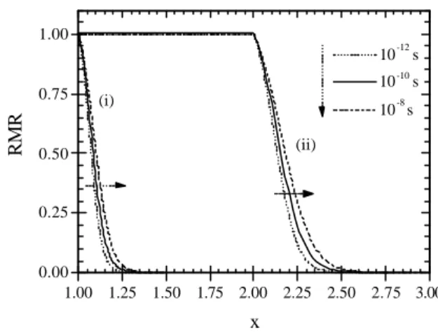
then calculating the logarithmic slopes at a given time, usually 1000s after the field change, and normalizing them by the slopes measured without a pulse to obtain RMR(x). We show the results of such calculations in Fig. 4, where two scenarii, thermal activation and QTM, have been considered. The case (i) correspond to the thermal activation scenario, for which T*(T)=T. Three calculated RMR curves are plotted, corresponding to three very different choices of P(U)∆m(U): 1/U5, U and U5. It is

obvious that the resulting variations in RMR are extremely small compared to the variations of S(T) showed in Fig.2. The corresponding RMR curves are indeed almost superimposed, thus emphasizing the main point of using this

procedure: step out of the unknown energy barrier distribution problem.

Let us now examine the quantum case (ii), where T*(T) becomes constant below a cross-over temperature of 1K, and a measurement temperature T0=0.5K is chosen.

The RMR is flat equal to 1 up to x=2. This is simply because the temperature pulse does not exceed the crossover temperature, and the relaxation rate is therefore not affected at all. At x=2, the temperature pulse begins to tackle the region of the crossover, and the residual relaxation rate after the pulse rapidly drops with the pulse height. That is why the calculated RMR shows this steep decrease after x=2. Moreover, the RMR is, as in case (i), quasi-insensitive to the three extreme variations of P(U)∆m(U) we considered. This shows that while RMR is very decoupled from P(U)∆m(U), it allows a clear distinction between QTM and thermal activation.

1.0 1.5 2.0 2.5 3.0 0.0 0.5 1.0 T * ( K ) T ( K ) ( i ) ( i i ) T₀ = 0.5 K T _cr = 1 K U U +5 U - 5 RMR x 0 1 2 0 1 2 ( i ) ( i i )

Fig. 4. Calculated RMR(x) for (i) thermally activated dynamics and (ii) quantum dynamics (in the plateau hypothesis with an arbitrary choice of Tcr=1K and

T0=0.5K). The corresponding effective temperatures are

plotted in the insert. Three choices of P(U)∆m(U) are represented.

We also performed numerous estimates of the sensitivity of RMR to some potentially not very well known quantities, such as the prefactor in the Néel-Brown expression of the relaxation time. The attempt time τ0is a slowly varying

function of the temperature, and we have checked the effect of such variations on the RMR.

In Fig. 5, we show how RMR weakly depends on the value of τ₀, since the curves, in both thermal activation (i) and QTM (ii) case, show little variation for τ0values ranging from 10-12 to 10-8 seconds. This shows that our procedure essentially probes the exponential term in the relaxation time, and is not very sensitive to the value of the attempt time.

1.00 1.25 1.50 1.75 2.00 2.25 2.50 2.75 3.00 0.00 0.25 0.50 0.75 1.00 (ii) (i) 10-12 s 10-10 s 10-8 s RMR x

Fig. 5. Variation of the calculated RMR in the thermal (i) and quantum (ii) cases for various very different values of the attempt time τ0.

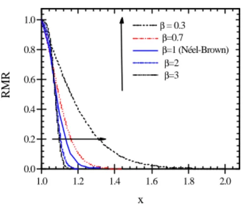
Another point that we wish to emphasize is the weak sensitivity of RMR to a departure from a Néel-Brown expression of the relaxation time for the activated dynamics. Some experimental results obtained on isolated monodomain magnetic nanoparticles showed a departure from this expression: the non-switching probability was fitted by exp[(-t/ τ)β], with β equals 1 for the Néel-Brown expression [9, 10]. The reported values of β are ranging from 0.3 to 7.

Fig. 6 shows the computed RMR for a few values of β, after the corresponding modification of the previous expression of m(t,T0,x).

1.0 1.2 1.4 1.6 1.8 2.0 0.0 0.2 0.4 0.6 0.8 1.0 β = 0.3 β=0.7 β=1 (Néel-Brown) β=2 β=3 RMR x

Fig. 6. Variation of the calculated RMR for various values of the parameter β.

One can see that the overall effect is small. In the case of β<1 (stretched exponential), the fall of RMR is smoother but RMR is already almost zero at x=1.6 in the extreme case

β=0.3. Moreover, the physical reason usually

invoked to explain this stretched exponential behavior is precisely the existence of a multi-valley energy landscape, for instance related to complex surface spin configurations. Actually, the RMR method already accounts for a barrier distribution, whatever its origin, and it does not seem clear to us that the use of β≠1 is justified in our calculations.

On the other hands, in the case β>1, the RMR falls off even faster than in the Néel-Brown case, and the contrast with a QTM-case RMR will not be affected.

After this review of the principle and virtues of the Residual Memory Ratio procedure, we will present some actual data acquired on two samples: one of moderate anisotropy (maghemite, γ-Fe2O3), and the other of high

anisotropy (cobalt ferrite, CoFe2O4) magnetic

nanoparticles.

3. Presentation of the samples

3.1. Maghemite (γ-Fe2O3)

The maghemite nanoparticles were chemically synthesized by following the protocol developed

by R. Massart [11] to prepare ferrofluids by coprecipitation. The sizes can be varied between 3 and 20 nm by tuning the temperature, the pH of the solution, or the proportions of the reactants. For typical diameters below 15 nm, the electrostatic repulsion linked to the surface charge avoids the aggregation of the particles that would result from the magnetic and Van der Waals interactions. The γ-Fe2O3 particles were then

embedded in a silica matrix by a room temperature polymerization process [12]. The X-ray diffraction patterns, as well as high-resolution TEM and Mössbauer spectroscopy confirmed that the particles were γ-Fe2O3. The

size distribution, determined after counting a sample of 440 particles on TEM micrographs, follows a lognormal law:

(

)

with a peak diameter d0=7nm and a standard

deviation

σ

The samples that we studied were extremely diluted (as low as 0.02% volume fraction), in order to minimize the interparticle interactions. Fig. 7 shows the zero-field cooled (ZFC) and field-cooled (FC) magnetic moments measured in 20Oe on a 0.021% volume fraction sample. We actually checked for a variety of concentrations, including all those mentioned in this article, that the FC and ZFC magnetization curves were very well superimposed when normalized to the volume fractions of magnetic nanoparticles. This clearly shows that magnetic interactions are indeed negligible.

Besides, magnetic hysteresis measurements at 1.9K yield an estimate of the anisotropy energy density K~2.105 erg/cm3, which is believed to allow a cross-over to a QTM regime below a few tenth of a Kelvin.

0 100 200 300 0.0

0.5 1.0

1.5 Zero Field Cooled (ZFC) Field Cooled (FC) H=20 Oe

M (10

emu )

T (K)

Fig. 7. Example of zero-field cooled (ZFC) and field-cooled (FC) magnetic moments measured for the maghemite sample (0.021% volume fraction).

3.2 Cobalt ferrite (CoFe2O4)

The Cobalt ferrite nanoparticles were prepared and characterized in a similar manner as the maghemite, by chemical coprecipitation. Their size distribution can be approximated by a lognormal law, with d0=5.3 nm and

σ

We show on Fig. 8 the ZFC-FC moments for a 0.012% sample, as well as one for the 2.3% sample of which we will present the relaxation data in section 4. One sees that there is a clear difference in shape, likely to be due to the non-negligible magnetic dipolar interactions in this more concentrated sample.

Finally, magnetic hysteresis measurements lead to K~4.106 erg/cm3, which roughly translate to a cross-over temperature of a few Kelvin, much higher than for the maghemite.

0 50 100 150 200 250 0.0 1.0 2.0 3.0 4.0 x_v=1.2 10-2 % x_v~2.3 % rescaled M/H ( 10 -6 cgs ) T ( K )

Fig. 8: ZFC and FC for two concentrations of CoFe2O4

particles. The 2.3% curve is rescaled for clarity.

4. Relaxation experiments: viscosity and RMR

4.1. Maghemite samples

4.1.1 Standard viscosity measurements

We first measured the relaxation properties by using the usual viscosity procedure, in two variants. The first one, that we will call “low-field”, is the following: the samples are cooled in a field of 60Oe, then the field is immediately switched to 0Oe and the magnetic moment is measured as a function of time. For γ-Fe2O3,

we also used a second procedure, that we will refer to as “high-field”, in which we prepare the samples by applying a –2000Oe field, strong enough to overcome all the energy barriers and put the magnetic moments of the particles to relax in the same hemisphere. We then sweep this field to some value H1,

between -100Oe and +1500Oe. Some particles relax during this step, and we wait 1 hour, mainly for damping the flux drift in the superconducting magnet. We then increase rapidly the field from H1 to H2=H1+46Oe by

using a copper coil, to trigger the relaxation processes that we want to analyze. The main

interest in using the “high-field” procedure is to reduce the energy barriers with the field, thus enabling us permitting to measure bigger particles. From estimates based on the value of the anisotropy energy density and the use of the Stoner-Wohlfarth model [13], the typical size of the particles that we see relaxing at 1 Kelvin would be 2nm with the “low-field” procedure. Under a magnetic field, it is possible to bring larger particles in the measurement window, and increasing the field allows us to scan an effective energy barrier distribution, which peaks for a certain value of the magnetic field. At the corresponding peak in the viscosity, the typical size of the relaxing particle is estimated to be around 9 nm, which is actually a little higher than the typical diameter 7nm.

Fig.9 shows the temperature dependence of the magnetic viscosity measured using the “low-field” procedure. Below 150mK , S(T) presents a striking upturn. It may be due to the presence of numerous small energy barriers, or to a quantum nature of the dynamics, or most likely to a combination of both as in a simple scenario of QTM one would not expect S(T) to increase back towards low temperatures.

0.0 0.2 0.4 0 20 40 S ( a . u . ) T ( K ) 0 1 2 3 4 5 0 200 400 600 800 S = d M / d ln(t) ( a.u. ) T ( K )

Fig.9. Magnetic viscosity as a function of the temperature for the maghemite sample after switching of a 60 Oe magnetic field (“low-field” procedure). The insert shows a detail of the upturn at very low temperature.

We then measured viscosity data using the “high-field” procedure, as shown on Fig.10. We also had to use a slightly less diluted sample (volume fraction 0.33%) to dominate a random background signal due to flux drifts in the superconducting magnet coupling to the SQUID pick-up coils.

0 500 1000 1500 0 2 4 6 8 0.1 K 0.3 K 1 K 3 K S ( 10 -4 emu/decade) H ( Oe )

Fig.10.Magnetic viscosity as a function of the final magnetic field for the maghemite sample at various temperatures. The dashed lines are guides for the eye.

All the measured curves S(H) show a maximum, related to the modulation of the energy barrier distribution by the magnetic field, which allows to scan the size distribution of the particles. The peak shifts towards higher fields as the temperature is lowered. At 100mK, we reach a different regime, and the curve peaks at a lower field. We found that this was due to some avalanches: the Zeeman energy released during the relaxation is enough to heat up the sample, thus generating more relaxation and even more heat. Careful measurements allowed us to ensure the reproducibility of such processes and we verified that, after waiting for one hour after the avalanche at 100mK, we were achieving a reproducible initial state before applying the 46Oe field variation and measuring the relaxation.

To be able to probe the nature of the dynamics, we then used the RMR method that has been discussed in Section 2. Fig. 11 shows the RMR data for the 0.041% volume fraction maghemite sample measured by using the “low-field” procedure. 1.0 1.5 2.0 2.5 3.0 0.0 0.5 1.0 0.06 K 0.1 K 0.5 K 1.0 K 2.0 K 3.0 K RMR x

Fig. 11. Measured RMR for a maghemite sample (0.041% volume fraction) using the “low-field” procedure. The solid line is the RMR predicted for thermally activated dynamics. The dashed lines are guides for the eye.

The RMR data at 3K and 2K fall very close to what is expected in the case of thermally activated dynamics. At lower temperatures, a clear departure from the thermal dynamics prediction is observed. These deviations are increasing with decreasing temperatures.

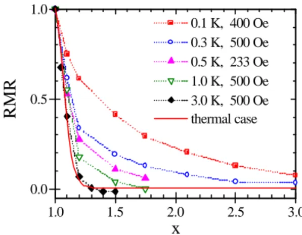
Fig. 12 shows the RMR measured using the “high-field” procedure for the 0.33% maghemite sample. The chosen values of the final field are close to those of the peaks in the viscosity curves of Fig.10. Then again the RMR at 3K is very close to the thermal prediction, but clearly departs from it when the temperature is lowered, in a very similar manner as for the “low-field” measurements. This is important to note, as we expect to probe very different sizes by using those two procedures: about 2nm diameter at 1K for the “low-field”, and about 9nm for the “high-field”, which means a factor roughly five in the

surface to volume ratios. This is a hint that those deviations are intrinsic to the nature of our particles, and probably not driven by their surface properties. Moreover, these deviations are fairly smooth compared to the RMR plateau of the QTM scenario curve of Fig. 4. In our opinion, this suggests a broad distribution of cross-over temperature, due for instance to a distribution in the anisotropy energy densities of the maghemite nanoparticles.

1.0 1.5 2.0 2.5 3.0 0.0 0.5 1.0 0.1 K, 400 Oe 0.3 K, 500 Oe 0.5 K, 233 Oe 1.0 K, 500 Oe 3.0 K, 500 Oe thermal case RMR x

Fig. 12 RMR measured using the “high-field” procedure for a maghemite sample (0.33% volume fraction). The dashed lines are guides for the eye.

4.2 Cobalt ferrite samples

4.1.2. Standard viscosity measurements

We measured the magnetic viscosity by using the “low-field” procedure previously introduced. Due to the lower relaxation signal (probably related to the high coercivity of those particles) we had to use a more concentrated sample, having 2.4% volume fraction of magnetic material. We also had to increase the fields for the “high-field” procedure, which yielded much higher flux drifts in the superconducting magnet, and prevented us from getting reproducible results. We will therefore present only the data obtained by using the “low-field” procedure. Fig. 13 shows the measured magnetic viscosity. It does not show the upturn we observed for the

maghemite sample, but the viscosity does not extrapolate to zero at low temperatures. Once again, this may mean either that the system crosses over to QTM like dynamics, or simply that many low energy barriers are present, in the form of small particles, surface spin configurations, etc. Applying the same logic as above, we then measured the RMR data to selectively sense the nature of the dynamics.

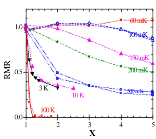
4.2.2. Residual Memory Ratio measurements

Our RMR data on the cobalt ferrite sample is reported on Fig. 14. Looking at the low temperature, we actually observe at 60mK and 100mK what we expect for QTM like dynamics: RMR stays flat equal to 1, even for temperature pulses as high as four or five times the initial temperature. At higher temperatures, RMR starts to fall off very rapidly initially, in a thermally activated fashion. But we observe here an effect that was not present in the

0 1 2 3 4 0 2 4 6 8 10 12 S (10 -6 emu / decade ) T ( K )

Fig. 13. Magnetic viscosity as a function of the temperature for the cobalt ferrite sample (2.4% volume fraction). The “low-field” procedure has been used.

maghemite samples: after this initial fast drop, the RMR does not fall to zero as we would expect from our simple model. On the contrary, it flattens off at about 0.2. We observed this effect up to relatively high temperature (over 10K), using a commercial SQUID magnetometer. As is shown on the graph, things eventually come back to normal at higher

temperatures: the 100K curve is very close to the prediction for thermal activation.

1 2 3 4 5 0.0 0.5 1.0 100 K 10 K 3 K _{500 mK} 200 mK 150 mK 100 mK 60 mK RMR X

Fig. 14. RMR results on the cobalt ferrite sample (2.4% volume fraction). The “low-field” procedure was used. The dashed lines are guides for the eye.

5. Discussion

The present data is obviously not compatible with the simplest case of independent thermally activated relaxation processes. Much more than the viscosity results, it is the RMR data that legitimates this first simple statement. We indeed observe two different kinds of strong deviations from this simplest case, for two different samples of very different anisotropy energy densities and concentrations. The cobalt ferrite sample shows a striking QTM-like plateau in its RMR below 150mK, but it is also a more concentrated sample, for which dipolar interactions are certainly not negligible anymore. On the other hand, it seems very difficult to attribute such deviations to the effect of magnetic interactions. In most interaction models (e.g. Dormann et al. [14]), the individual energy barrier of one given particle is enhanced by the dipolar interactions with neighboring particles, thus leading to some kind of collective freezing and to an increase in its energy barrier as the temperature is lowered. In spin-glasses, for example, the barriers are known to increase as the

temperature is lowered [15], and one would therefore expect to see the opposite deviation on RMR: during the temperature pulse, the barriers will be lowered and accordingly easier to overcome than if in the non-interacting case. The expected RMR would therefore fall faster then the curves we show for thermal activation, which is the opposite of what we observe. We actually did measure RMR data on a spin-glass sample CdCr1.7In0.3S4 at 12K, i.e. below

its freezing temperature of 16.7K. The results, presented in Fig. 15, show that the RMR is indeed falling faster than for the “no-interactions” thermal activation prediction

1.0 1.2 1.4 1.6 1.8 2.0 0.0 0.2 0.4 0.6 0.8 1.0 _CdCr 1.7In0.3S4 T=12K no-interactions prediction RMR x

Fig. 15. Measurement of RMR for a CdCr1.7In0.3S4

spin-glass sample at 12K. The deviations from the non-interacting thermal activation case are opposite to those we observe for the nanoparticles. The dashed lines are guides for the eye.

The RMR data we measured on the cobalt ferrite yields another issue. The RMR procedure assumes that the energy barrier distribution P(U)∆m(U) is temperature independent. In the cobalt ferrite sample, we do not understand why RMR levels-off at 0.2, up to relatively high values of x, in spite of a sharp “thermal activation” like initial decrease as seen in Fig. 14 at temperatures above 3K. One reason we may think of is that at very small values of x, we probe the dynamics in a “non-destructive” way, where the physical properties

of the particles are not changing much and P(U)∆m(U) is really independent of the temperature. On the contrary, at larger values of x, P(U)∆m(U) may start to be affected, because some physical properties are: the effective anisotropy energy density, or the magnetization, of the nanoparticles may vary due their small size and/or defects, since this is of course not expected in the bulk materials. It is then conceivable that the barriers should increase during the temperature pulse, thus preventing the RMR from dropping to zero as it should. We can therefore check our conclusions by only considering the data at small x. Following this idea, we analyzed the data by considering the initial angle (both RMR and x being dimensionless) of the curves with the horizontal. As shown in Fig. 16, a pure QTM behavior would then correspond to a zero degree angle, whereas the thermally activated dynamics would show up as an angle of roughly –80 degrees. 1.0 1.5 2.0 2.5 3.0 0.0 0.5 1.0 data thermal quantum RM R AN GLE (x<1.2) RMR x

Fig. 16. Principle of the “Initial-angle” analysis for the RMR data

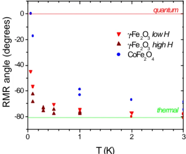
Using such a method, we can summarize the present data in Fig. 17, which clearly supports a crossover from thermally activated to QTM dynamics for both the maghemite and the cobalt ferrite. Interestingly enough, the behavior is not noticeably different between the

“low-field” and “high-field” procedures for the maghemite sample, in spite of the very different sizes of particles that we have in the measurement window (respectively 2nm and 9nm), which suggests an intrinsic origin to this quantum behavior. Last but not least, for the cobalt ferrite, this crossover happens at a much higher temperature than for the maghemite, which is in agreement with the much higher anisotropy energy density of the cobalt ferrite nanoparticles. 0 1 2 3 -80 -60 -40 -20 0 thermal quantum γ-Fe₂O₃ low H γ-Fe₂O₃ high H CoFe 2O4 RMR angle (degrees) T (K)

Fig. 17. Summary of the RMR data analyzed using the initial- angle analysis.

6. Conclusion

We have recalled how magnetic viscosity measurements are by essence mixing the nature of the dynamics with the distribution of energy barriers. We have developed and used as a complement the “Residual Memory Ratio” (RMR) method. This relaxation procedure enables us to eliminate the sensitivity to the energy barrier distribution, thus providing a reliable insight on the nature of the observed dynamics. By using a custom made apparatus coupling dilution refrigeration and SQUID magnetometry, we have performed measurements of very diluted samples at temperatures as low as 60mK. Two types of particles have been studied: γ-Fe2O3 of

moderate anisotropy, and CoFe2O4 of higher

anisotropy where quantum effects are likely to occur at higher temperatures. In both cases, the data showed a clear departure from the predictions for RMR in thermal activation regime.

For the cobalt ferrite, a QTM-like plateau is even reached in the RMR below 150mK, but at higher temperatures we do not fully understand the RMR for high values of x. The situation is probably more complicated than for the maghemite, as the higher volume fraction we used yields non-negligible magnetic dipolar interactions. Nevertheless, these deviations go the opposite way of what is expected from the effect of particles magnetic interactions, thus giving us confidence that the low temperature and low x data is still very supportive of QTM. In the case of the maghemite, the situation is even clearer because of the RMR does behave as expected in a thermal way at high temperatures and high x, and clearly deviates from the prediction for thermally activated dynamics at 100mK and below. Moreover, the same behavior is observed in the “high-field” and “low-field” procedures, thus showing an intrinsic origin to this behavior, and pointing to a smooth crossover to a QTM regime at very low temperatures.

Acknowledgments

This research was entirely performed at the Service de Physique de l’Etat Condensé (SPEC), CEA Saclay, France. We wish to thank P. Pari, P. Bonville L. Le Pape, and P. Forget for their scientific or technical assistance at the SPEC. The authors are also very grateful to F. Chaput and J.P. Boilot (PMC, Ecole Polytechnique, Palaiseau, France), D. Zins and S. Neveu (Laboratoire de Physico-Chimie Inorganique, Université Pierre et Marie Curie, Paris, France) for the preparation of the magnetic nanoparticles.

1

E.M. Chudnovsky and L. Gunther, Phys. Rev. Lett. 60 (1988) 661

2

M. Enz and R. Schilling, J. Phys. C 19 (1986) L711

3

G. Scharf, W.F. Wreszinski and J. L. Van Hemmen, J. Phys. A (1987) 4309

4

W. Wernsdorfer, E. Bonet Orozco, K. Hasselbach, A. Benoit, D. Mailly, O. Kubo, H. Nakano and B. Barbara, Phys. Rev. Lett. 79 (1997) 4014

5

B. Barbara, L.C. Sampaio, A. Marchand, O. Kubo and H. Takeuchi, J. Magn. Magn. Mater. 136 (1994) 183

6

R. Sappey, E. Vincent, M. Ocio, J. Hammann, F. Chaput, J.P. Boilot and D. Zins, Europhys. Lett. 37 (1997) 639

7

M. Uehara, B. Barbara, J. Physique 47 (1986) 235

8

R.H. Kodama, A.E. Berkowitz, E.J. McNiff Jr., and S. Foner, Phys. Rev. Lett. 77 (1996) 394

9

M. Lederman, S. Schultz and M. Oszaki, Phys. Rev. Lett. 73 (1994) 1986

10

W. Wernsdorfer, K. Hasselbach, D. Mailly, B. Barbara, A. Benoit, L. Thomas and G. Suran, J. Magn. Magn. Mater. 145 (1995) 33

11

R. Massart, IEEE Trans. Magn. 17 (1981) 1247

12

F. Devreux, J.P. Boilot, F. Chaput and A. Lecompte, Phys. Rev. A 41 (1990) 6901

13

E.C. Stoner and E.P. Wolhfarth, Philos. Trans. London Ser. A 240 (1948) 599

14

J.L. Dormann, L. Bessais and D. Fiorani, J. Phys. C 21 (1988) 2015

15

J. Hammann, M. Lederman, M. Ocio, R. Orbach and E. Vincent, Physica A 185 (1992) 278; E. Vincent, J. Hammann, M. Ocio, J.-P. Bouchaud and L. Cugliandolo, in "Complex Behaviour of Glassy Systems", Springer Lecture Notes in Physics Vol.492, Editor M. Rubi, (1997) 184 (preprint cond-mat/9607224).