HAL Id: halshs-00671378
https://halshs.archives-ouvertes.fr/halshs-00671378
Preprint submitted on 17 Feb 2012
HAL is a multi-disciplinary open access archive for the deposit and dissemination of sci-entific research documents, whether they are pub-lished or not. The documents may come from teaching and research institutions in France or abroad, or from public or private research centers.
L’archive ouverte pluridisciplinaire HAL, est destinée au dépôt et à la diffusion de documents scientifiques de niveau recherche, publiés ou non, émanant des établissements d’enseignement et de recherche français ou étrangers, des laboratoires publics ou privés.
Do We Follow Private Information when We Should?
Laboratory Evidence on Naive Herding
Christoph March, Sebastian Krügel, Anthony Ziegelmeyer
To cite this version:
Christoph March, Sebastian Krügel, Anthony Ziegelmeyer. Do We Follow Private Information when We Should? Laboratory Evidence on Naive Herding. 2012. �halshs-00671378�
WORKING PAPER N° 2012 – 07
Do We Follow Private Information when We Should? Laboratory
Evidence on Naive Herding
Christoph March
Sebastian Krügel
Anthony Ziegelmeyer
JEL Codes: C91, D82, D83
Keywords: Information Cascades, Laboratory Experiments, Naive Herding
P
ARIS-JOURDANS
CIENCESE
CONOMIQUES48, BD JOURDAN – E.N.S. – 75014 PARIS TÉL. : 33(0) 1 43 13 63 00 – FAX : 33 (0) 1 43 13 63 10
www.pse.ens.fr
Do We Follow Private Information when We Should?
Laboratory Evidence on Na¨ıve Herding
∗Christoph March†, Sebastian Kr¨ugel‡ and Anthony Ziegelmeyer§
This version: January 26, 2012
Abstract
We investigate whether experimental participants follow their private information and contradict herds in situations where it is empirically optimal to do so. We consider two sequences of players, an observed and an unobserved sequence. Observed players sequentially predict which of two options has been randomly chosen with the help of a medium quality private signal. Unobserved players predict which of the two options has been randomly chosen knowing previous choices of observed and with the help of a low, medium or high quality signal. We use preprogrammed computers as observed players in half the experimental sessions. Our new evidence suggests that participants are prone to a ‘social-confirmation’ bias and it gives support to the argument that they na¨ıvely believe that each observable choice reveals a substantial amount of that person’s private information. Though both the ‘overweighting-of-private-information’ and the ‘social-confirmation’ bias coexist in our data, participants forgo much larger parts of earnings when herding na¨ıvely than when relying too much on their private information. Unobserved participants make the empirically optimal choice in 77 and 84 percent of the cases in the human-human and computer-human treatment which suggests that social learning improves in the presence of lower behavioral uncertainty.
1
Introduction
With the help of a large meta-dataset covering 13 experiments on social learning games, Weizs¨acker (2010) investigates whether participants follow others and contradict their private information in situations where it is empirically optimal to do so. Weizs¨acker finds that participants are quite unsuccessful in learning from others. The average participant follows others only in situations where the evidence conveyed by their observable choices is so strong that the private information is wrong more than twice as often as it is correct. Economic experiments on social learning games have repeatedly concluded that Bayesian rationality organizes well most of participants’ choices except for an inflated tendency to follow private information (among others, N¨oth and Weber, 2003; Goeree, Palfrey, Rogers, and McKelvey, 2007). By estimating the value of the available actions, the meta-study additionally shows that participants forgo substantial parts of earnings when falling prey to the ‘overweighting-of-private-information’ bias.
∗
The first author gratefully acknowledges financial support from the European Research Council.
†
Corresponding author: Paris School of Economics, 48 Boulevard Jourdan, 75014 Paris, France. Email:
‡
Max Planck Institute of Economics, IMPRS “Uncertainty”, Kahlaische Strasse 10, D-07745 Jena, Germany. Email: [email protected].
§
Max Planck Institute of Economics, Strategic Interaction Group, Kahlaische Strasse 10, D-07745 Jena, Germany. Email: [email protected].
The bulk of Weizs¨acker’s meta-dataset consists of experimental treatments that implement the stripped-down model of information cascades developed by Bikhchandani, Hirshleifer, and Welch (1992, henceforth BHW). In this simple social learning environment, a sequence of participants each in turn choose one of two options with each participant observing all of her predecessors’ choices. Induced preferences over the two equally likely options are common, and participants receive independent and equally strong private binary signals about the correct option. According to Bayesian rationality, once the pattern of signals leads to two identical choices not canceled out by previous ones, all subsequent participants should ignore their signals and follow the herd. Though of interest, the experimental evidence on social learning behavior provided by the existing literature is too restrictive. Of particular concern is the coarseness of the social learning environment which favors the emergence of the ‘overweighting-of-private-information’ bias.1
In this paper, we investigate whether participants follow their private information and contradict herds in situations where it is empirically optimal to do so. To address this complementary issue, our social learning game relies on a richer information structure than BHW’s stripped-down model. Following Ziegelmeyer, Koessler, Bracht, and Winter (2010), we consider two sequences of players, an observed and an unobserved sequence. Observed players sequentially predict which of two options has been randomly chosen with the help of a medium quality private signal (quality equals 14/21). At the end of each decision period, the choice of one observed is made public knowledge. In a matched pairs design, unobserved players guess which of the two options has been randomly chosen knowing previous public choices and with the help of a low, medium or high quality signal (quality equals 12/21, 14/21 or 18/21 respectively). Their choices remain private.
Our laboratory experiment uses an expanding strategy method-like procedure that allows us to detect herding behavior directly, allows participants to gain experience with many decision nodes, and generates a large dataset (see also Cipriani and Guarino, 2009). In the first part of each session, the signal’s quality for the unobserved is fixed at the beginning of each of the three rounds, each player observes only one signal realization and makes only one choice. Each participant earns 0.4 (0.1) Euro for each correct (wrong) guess. The second part of each session is identical to the first part except that i) all unobserved make one choice in each decision period (8 choices in total); ii) all seven observed make one choice in decision period 1 and one choice is randomly selected to be made public, the remaining six observed make one choice in decision period 2 and one choice is randomly selected to be made public, and so on till decision period 7 where the remaining observed makes a last choice; and iii) for each participant, only one randomly selected choice is paid in each round. The third part of each session is identical to the second part except that each choice is made for both realizations of the private signal. Players are informed of the payoff-relevant realization of their private signal after having made their last choice. Finally, the fourth part of each session is identical to the third part except that i) there are six rounds; ii) unobserved make their choices for each quality of the private signal and they are informed of the payoff-relevant quality of their private signal at the end of each round; and iii) for each participant, only one randomly selected choice is paid and each participant earns 12 (3) Euro for a correct (wrong) guess.
A second novelty of our design is the use of preprogrammed computers as observed players in three out of the six experimental sessions. Unobserved players, on the other hand, are always embodied by
1
In situations where predecessors’ choices do not point in any direction or point in the same direction as private information, following private information seems the only reasonable choice. In these situations, the few experimental choices not in line with private information have been understood as resulting from confusion. Moreover, in situations where an option is favored by exactly one choice over the other option and private information points in the opposite direction, Bayesian rationality is silent about the optimal choice. Note that about one third of the data in Weizs¨acker’s meta-dataset stem from N¨oth and Weber (2003) which considers two privately known signal precisions. However, the predictions in this variant of BHW’s stripped-down model closely match the original ones.
human participants. Though the computers’ strategy is not revealed to the unobserved participants, the latter face lower behavioral uncertainty in the computer-human treatment than in the human-human treatment and, no matter how big the contradicting herd is, it is always beneficial for them to follow their high quality signal. Our dataset contains 1,827 choices from 21 observed participants, 8,712 choices from 24 unobserved participants in the human-human treatment, and 8,712 choices from 24 unobserved participants in the computer-human treatment. Given the experimental choices of the observed participants, the estimation of the empirical value of actions leads to the conclusion that following the high quality signal is also the empirically optimal action for the unobserved participants in the human-human treatment no matter how big the contradicting herd is.
The richness of our dataset enables us to measure the success of social learning both in situations where it is empirically optimal to follow others (and contradict private information) and in situations where it is empirically optimal to follow private information (and contradict the herd).2 We infer
that, conditional on being endowed with a low or medium quality signal and observing a contradicting herd of size at least 2, participants make the empirically optimal choice in 75 percent of the cases. In contrast, conditional on being endowed with a high quality signal and observing a contradicting herd of size at least 2, unobserved participants choose optimally in only 56 percent of the cases. In the latter situations, the evidence conveyed by the observable choices is so weak that the private information is correct more than twice as often as it is wrong. Our new evidence therefore suggests that participants are prone to a ‘social-confirmation’ bias and it gives support to the argument that they na¨ıvely believe that each observable choice reveals a substantial amount of that person’s private information (Eyster and Rabin, 2010). Though both the ‘overweighting-of-private-information’ and the ‘social-confirmation’ bias coexist in our data, participants forgo much larger parts of earnings when herding na¨ıvely than when relying too much on their private information. Finally, compared to the human-human treatment, we observe slightly less na¨ıve herding and slightly more overweighting-of-private-information in the computer-human treatment. Overall, unobserved participants make the empirically optimal choice in 77 and 84 percent of the cases in the human-human and computer-human treatment which suggests that social learning improves in the presence of lower behavioral uncertainty.
The next section describes the experimental design and practical procedures. Section 3 derives the relevant theoretical predictions. Section 4 presents our experimental results. Section 5 concludes. The supplementary material contains a translated version of our instructions.
2
The Experiment
In our information cascade experiment participants make binary decisions in sequence encumbered solely by state-of-Nature uncertainty, and they may condition their decisions both on private signals about the state of Nature and on some earlier decisions. Participants make informational inferences in many analogous situations distinguished by either the history of previous choices, the quality or the realization of the private signal. The experimental setting therefore allows participants to gain extensive experience with the combination of private and public information while offering at the same time the unique chance to carefully study social learning behavior at the individual level.
Our setting builds upon three main ingredients.
2
We rely on a modified version of Weizs¨acker’s (2010) counting technique to estimate the value of contradicting private information.
Observed and Unobserved Players
The experimental social learning game involves observed and unobserved players. Each repetition of the game begins with the random selection of one of two options which remains hidden to the players. The latter obtain independent private signals that reveal information about which of the two options has been randomly selected. Binary private signals for observed are of medium quality whereas the signal quality for unobserved is either low, medium or high. Players choose in sequence one of the two options, and the monetary payoff is larger for a correct prediction than for an incorrect prediction. Once all choices have been submitted in a given decision period (but the last one), the choice of one observed is made public knowledge. The choices of unobserved remain private. Participant keep the same role of observed or unobserved during the entire experimental session.
Increasing Reliance on the Strategy Method
Our experiment consists of four parts with later parts relying more on the strategy method than earlier ones. In each repetition of the game, 7 observed and 8 unobserved make choices over 8 decision periods.
In the first part of the experiment, participants gain direct-response experience with the social learning game. Each player is endowed with only one realization of the private signal and makes exactly one choice in each of the three repetitions of the game. Concretely, observed obtain a single draw from an urn containing 14 balls indicative of the randomly selected option and 7 balls indicative of the other option (hereafter, simply correct and incorrect balls). Unobserved obtain a single draw from an urn containing 14 (18 and 12) correct balls and 7 (3 and 9) incorrect balls in the first (second and third) repetition, respectively. In each of the first seven decision periods, one observed and one unobserved chooses one of the two options. In the last decision period, only the remaining unobserved makes a choice. Assignments to decision periods are random. From the second decision period on, players may condition their choices on the choices made by observed in previous decision periods. Participants receive 0.4 Euro for a correct prediction and 0.1 Euro otherwise.
The second part of the experiment is identical to the first one except that each unobserved makes 8 choices and each observed makes between 1 and 7 choices in each of the three repetitions of the game. In the first decision period, all 15 players choose one of the two options. The choice of one observed is randomly selected to be made public at the beginning of the next period and this player stops from making predictions. In the second decision period, all remaining 14 players choose one of the two options. The choice of one observed is randomly selected to be made public at the beginning of the next period and this player stops from making predictions. And so on, until the last decision period where all unobserved choose one of the two options. For each participant, only one randomly selected prediction is paid in each repetition.
The third part of the experiment is identical to the second one except that each choice is made for both realizations of the private signal. Players are informed of the payoff-relevant realization of their private signal after having made their last choice.
Finally, the fourth part of the experiment collects the largest number of contingent choices per repetition of the game. Though observed make on average the same number of contingent choices as in the previous part, unobserved choose one of the two options for each quality and realization of the private signal in each decision period. They are informed of the payoff-relevant quality and realization of their private signal after having made their last choice. Other differences with the previous part include the six repetitions of the game and the fact that participants receive 12 Euro for a correct
prediction and 3 Euro otherwise.3
Observed as Computers or Humans
We use preprogrammed computers as observed players in half the experimental sessions. Unobserved, on the other hand, are always embodied by human participants. In sessions where unobserved se-quentially learn from computers, they do so without knowing the computers’ strategy. The third main ingredient of our experiment serves two purposes. First, we facilitate social learning for the un-observed in sessions where they observe the choices of computers since the latter behave in a simple deterministic way as they adopt the Bayesian rational strategy (see Section 3.2.1). This exogenous variation in behavioral uncertainty enables us to check one of Weizs¨acker’s (2010) conclusion accord-ing to which participants make worse informational inferences in situations where public information is less clear. Second, in sessions where computers act as observed players, we can perfectly identify the empirically optimal action for unobserved at each decision node.
2.1 Treatments and Procedures
The experiment consists of the Computer-Human and Human-Human treatments. The two options from which one was randomly selected at the beginning of a repetition were labeled ‘BLUE’ and ‘GREEN’. Option ‘BLUE’ had a 11/20 probability to be selected and option ‘GREEN’ had a 9/20 probability to be selected. We conducted three sessions in each treatment. Most participants were students at the Friedrich Schiller University of Jena, and a few were students at the University of Ap-plied Sciences Jena. The experimental sessions took place at the Experimental Laboratory of the Max Planck Institute of Economics (ELMPIE) in Jena, and participants were invited using the ORSEE recruitment system (Greiner, 2004). Each session in the Computer-Human and Human-Human treat-ment involved 9 and 16 participants respectively, one participant being randomly selected to serve as the experimental assistant.
At the start of each session in the Human-Human treatment, experimenters demonstrated the option-selection procedure to small groups of participants. An experimenter shuffled a deck of 20 cards and laid them down on a table with the back of the cards facing the assistant. 11 cards had a blue front and 9 cards had a green front. The assistant then picked 1 card out of the 20 cards, the front color of the picked card determining the randomly selected option. Experimenters also showed to participants how the order of predictions was randomly determined in the first part of the experiment.
After the two demonstrations, paper instructions for part 1 were distributed and participants were given time to read them once at their own pace. Instructions were then read aloud, participants learned about their role (observed or unobserved ), and they answered a few control questions. Experimenters checked participants’ answers, and they explained mistakes privately to participants whenever needed. After that, part 1 was ran following the “balls and urns” procedure of Anderson and Holt (1997). In each of the three repetitions of the social learning game, participants were asked to fill in a form with the realization of their private signal, the choices they observed and the choice they made, and, once known, the option selected at random by the assistant.
The second part of the session was computerized. Electronic instructions detailed the course of
3Even in the last part of the experiment, our setting relies only on the partial strategy method. Indeed, for relatively
long decision-making sequences, the implementation of the full strategy method seems impractical in information cascade experiments. Participants would have to submit hundreds of predictions without ever becoming familiar with the environment. Moreover, long decision-making sequences are preferable since the main regularity observed in cascade experiments is the correlation of length and strength of laboratory herds (K¨ubler and Weizs¨acker, 2005).
the second part, and illustrations were provided concerning the random draw of the private signal, the implementation of choices and the feedback at the end of each repetition. A short summary of the instructions was read aloud. After that, the three repetitions of part 2 were ran.
The third and fourth parts of the session were conducted similarly to the second one except that short paper instructions replaced the electronic instructions. Participants were then asked to report their month and year of birth, their gender, and their academic major. Finally, participants privately retrieved their earnings.
Sessions in the Computer-Human treatment followed the same procedure except for the presence of preprogrammed computer algorithms. At the end of the session, participants had the possibility to earn 10 additional Euro by correctly identifying the strategy of computer algorithms.4
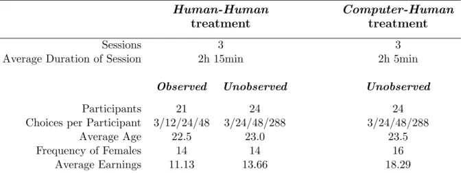
Table 1 summarizes our experimental treatments.
Human-Human Computer-Human
treatment treatment
Sessions 3 3
Average Duration of Session 2h 15min 2h 5min
Observed Unobserved Unobserved
Participants 21 24 24
Choices per Participant 3/12/24/48 3/24/48/288 3/24/48/288
Average Age 22.5 23.0 23.5
Frequency of Females 14 14 16
Average Earnings 11.13 13.66 18.29
Notes: In each column, the number of choices per participant is reported for the four different parts separately. In the last three parts, averages are reported for observed.
Earnings are stated in Euro and they include a show-up fee of 5 Euro which corresponds to twice the usual amount due to lengthy sessions. Earnings in the Computer-Human treatment do not include the 10 Euro earned by correctly identifying the strategy of computer algorithms.
Table 1: Experimental Design
3
Theoretical Considerations
In this section, we provide a formal description of our social learning game and the predictions of a series of behavioral models. First, we consider the full rationality model. The standard predictions are mainly derived to describe the behavior of the computer players in the Computer-Human treatment as the latter follow the Bayesian rational strategy. Second, we extend the standard approach by allowing noisy optimizing behavior while maintaining the internal consistency of rational expectations. The quantal response equilibrium approach has been considered in past studies as a first good approxima-tion to actual behavior in experimental social learning games (see especially Goeree, Palfrey, Rogers, and McKelvey, 2007), and we agree that the introduction of a random component in decision-making is a reasonable starting point. Still, the existing experimental literature has also established that the main regularities observed in laboratory cascades are not captured in a fully satisfactory way by the
4One pilot session was conducted in each treatment. We do not include these two pilot sessions since their structure
quantal response equilibrium. We therefore extend noisy best reply with rational expectations in two directions. On the one hand we allow for disequilibrium beliefs as argued by K¨ubler and Weizs¨acker (2004), and on the other hand we consider an equilibrium approach with non-Bayesian updating of beliefs. In the last part of this section, we illustrate the two final approaches to show that both have the potential to capture the full diversity of experimental regularities.
3.1 A Rich-Information Social Learning Game
There are two payoff-relevant states of Nature (henceforth states)—state B and state G, and two possible actions—“predict state B” simply denoted by B and “predict state G” simply denoted by G. Nature chooses state B with probability p = 11/20. The finite set of players is {1, . . . , N } with generic element n. For all players, action B has vN-M payoffs u (B, B) = 1 and u (B, G) = 0, and action G has vN-M payoffs u (G, B) = 0 and u (G, G) = 1.5
Nature moves first and chooses a state which remains unknown to the players. Each player is then endowed with a private signal which corresponds to the realization of a random variable, denoted by ˜sn, with support S = {b, g}, and whose distribution depends on the state. Conditional on the
state, private signals are independently distributed across players. In state B (resp. state G), player n receives signal b (resp. signal g) with probability p < qn < 1 and signal g (resp. signal b) with
probability 0 < 1 − qn < 1 − p. We refer to qn as player n’s signal quality. There are two groups
of players. Observed receive private signals of medium quality qn = 14/21 meaning that the signal
indicates the true state of Nature in two thirds of the cases. Private signals of unobserved have quality qn∈ {12/21, 14/21, 18/21}.
Time is discrete and, in each period t = 1, 2, . . . , T , k ≤ N players simultaneously choose an action. The action of exactly one observed is then publicly revealed at the beginning of the next decision-making period. The observed whose action is made public does not act in any subsequent period. Accordingly, players who act in period t ∈ {1, . . . , T } observe the history ht= (a1, . . . , at−1) ∈
Ht= {B, G}t−1where aτ is the action which is public in period τ ∈ {1, . . . , t − 1} and h1 = ∅. Payoffs
are realized at the end of period T such that observed receive the payoff from the action which is made public and unobserved receive the payoff from their action in exactly one randomly chosen period. Since payoff externalities are absent and we abstract from social preferences the game is similar to a social learning game where each player is randomly assigned to exactly one period and makes a once-in-a-lifetime decision.
For each player a belief for period t is given by the mapping µt: {b, g}×Ht→ [0, 1] where µt(sn, ht)
denotes the conditional probability assigned to state B given signal sn ∈ {b, g} and observed history
ht ∈ Ht. A behavioral strategy for period t is a mapping σt(sn, ht) : {b, g} × Ht → [0, 1] where
σt(sn, ht) denotes the probability that the player takes action B given signal sn and history ht. We
say that player n follows private information at history ht when taking action B with sn = b or
taking action G with sn = g. Alternatively, player n contradicts private information at history ht
when taking action B with sn= g or taking action G with sn= b.
3.2 Predictions
3.2.1 Perfect Bayesian Rationality
We first assume that players are Bayes-rational, and that Bayesian rationality and the structure of the game are commonly known. Under these assumptions the game has a unique rationalizable
5
Assuming well-behaved non-expected utility maximizers does not significantly alter the predictions of our behavioral models.
outcome. In period 1, observed follow private information. Consequently, in period 2, observed follow private information only if the history is G and they choose action B independently of their private information if the history is B. Hence, after action B is revealed at the beginning of period 2, an information cascade starts in which all subsequent observed choose action B.6 In a cascade, the
beliefs of two players are identical when endowed with the same private signal. A similar reasoning implies that an information cascade in which all observed choose G starts at history GG. More generally, a B-cascade (resp. G-cascade) starts after one public B (resp. two G) not canceled out by previous public actions. The only history which does not lead to an information cascade is the history GBGB . . . GB, and the probability that no cascade has started by period 2k + 1 decreases exponentially.
Unobserved with signal quality qn = 12/21 follow private information only in the first period
and in odd periods following history GB . . . GB, and otherwise they choose the action which has been publicly revealed most frequently. Obviously, unobserved with signal quality qn= 14/21 behave
similarly as observed. Finally, unobserved with signal quality qn = 18/21 follow private information
at all histories.
Notice that Bayes-rational players have a correct perception of the expected value of each action which implies that they follow (contradict) private information provided their belief is indicative of the same action as their signal with probability at least (at most) 1/2.
3.2.2 Almost Bayesian Rationality
We now derive predictions for the quantal response equilibrium model (McKelvey and Palfrey, 1995, 1998). We rely on the common logit specification given by
σtλ(sn, ht) =
h
1 + eλ (1 − 2 µt(sn,ht))i
−1
where λ ≥ 0 denotes players’ sensitivity to payoff differences. Choices are random if λ = 0, they become more responsive to beliefs as λ increases and players best respond to beliefs as λ → ∞.7
Assuming that the sensitivity to payoff differences is commonly known, player n’s belief at history ht with signal sn is given by
µt(sn, ht) = 1 + 1 − p p Pr (˜sn= sn| ˜ω = G) Pr (˜sn= sn| ˜ω = B) Y τ <t P sτ∈S Pr (sτ | G) στλ(aτ | sτ, hτ) P sτ∈S Pr (sτ | B) στλ(aτ | sτ, hτ) −1
where sτ and aτ are respectively the signal realization and the action of an observed whose action has
been made public. The dynamics of beliefs and choices have the following properties: First, each public action conveys a noisy signal about the state of Nature as σtλ(sn, ht) strictly increases with µt(sn, ht).
Actions reveal less information the noisier choice probabilities are (the smaller λ is). Second, since each action conveys some information each player is more likely to contradict than to follow private information after observing a large number of similar choices which point in the opposite direction of private information. Accordingly, “cascades” emerge and they do so no sooner than predicted by perfect Bayesian rationality. Even unobserved with high signal quality become more likely to contradict private information. Third, since no action is chosen with certainty (0 < σλt (sn, ht) for
each sn, qn, ht) a cascade once started is broken with strictly positive probability in each subsequent
period. Players who break a cascade are more likely to have a contradictory signal. Fourth, the
6Information cascades only develop in the observed sequence. 7
longer a cascade the more likely players are to contradict private information. Fifth, cascades are self-correcting meaning that after the break of an incorrect cascade the new cascade which emerges is often a correct one.8 Finally, players have a correct perception of the available information meaning that players contradict private information with probability at least 1/2 if and only if the expected payoff from contradicting is larger than the expected payoff from following private information.
3.2.3 Limited Bayesian Rationality
So far we assumed that players’ behavioral strategies are commonly known (or can be derived from commonly known traits). In general, a player’s belief with signal snat history ht is given by
µt(sn, ht) = 1 + 1 − p p Pr (sn| G) Pr (sn| B) Y τ <t P sτ Pr (sτ | G) ˆστ(aτ | sτ, hτ) P sτ Pr (sτ | B) ˆστ(aτ | sτ, hτ) −1
where Pr (˜sn= b | B) = Pr (˜sn= g | G) = qn and ˆστ(aτ | sτ, hτ) are the choice probabilities for signal
sτ and history hτ assessed by player n. If strategies are commonly known these probabilities coincide
with probabilities στ(aτ | sτ, hτ) where (with a slight abuse of notation) στ(B | sτ, hτ) = στ(sτ, hτ)
and στ(G | sτ, hτ) = 1 − στ(sτ, hτ).
The formation of correct beliefs through iterative reasoning is highly demanding from a cognitive point of view. We now discuss the dynamics of beliefs and choices under limited strategic thinking. We consider the level-k model (Stahl and Wilson, 1995) according to which each player is one of a (potentially infinite) number of types (L0, )L1, L2, . . .. Although players are heterogeneous, each
player’s type is drawn from a common distribution. Type Lk anchors its beliefs in a non-strategic
type L0 which captures instinctive responses to the game and adjusts them via thought-experiments
with iterated best responses. Concretely, type Lk noisy best responds to a belief formed under the
assumption that other players are of type Lk−1. We assume that the structure of the game and
quantal response functions are iteratively know up to level k for type Lk. Finally, we assume that
type L0 noisy best responds to private beliefs only.9
Consider first the case where players best respond to beliefs. L0 players ignore public information
and best respond to private information. L1 players therefore believe that each action perfectly
reveals the underlying signal and they form beliefs according to a counting rule.10 It is easy to see
that observed L1 players and unobserved L1 players with signal quality qn ∈ {12/21, 14/21} mimic
the behavior of Bayes-rational players. However, the beliefs of L1 players increase (decrease) with
the number of public B (G) choices which eventually leads unobserved L1 with high signal quality
qn = 18/21 to contradict private information. The latter is not true for Lk players such that k > 1.
Indeed, beliefs and choices of L2players are the same for all signal qualities as those of Bayes-rational
players.
Under noisy best reply, L0 players follow private information with probability at least 1/2, but
they occasionally make mistakes. Accordingly, L1 players infer from each public action a signal which
is noisier than the underlying private signal which leads them to form beliefs according to a counting rule with discounting. L1 players now follow private information (with probability at least 1/2) at
more histories. Contrary to almost Bayes-rational players, L1 players’ beliefs become extreme more
8See Goeree, Palfrey, Rogers, and McKelvey (2007) for a more precise characterization of the social learning outcome
in quantal response equilibrium.
9Assuming that L
0 players choose randomly implies that L1 respond to private beliefs and the subsequent analysis
carries over with the type hierarchy shifted upwards by one level.
10
quickly. For higher types differences are more subtle. For instance, L2 players correctly infer that the
second observed action conveys less (more) information if it matches (differs from) the first action. However, if the first three observed actions match they infer too little information from the third action assuming wrongly that the third player did not take into account the reduced information conveyed by the second action.
Notice that Lk players have an incorrect perception of the expected value of actions unless an
arbitrarily large fraction of the population is of type Lk−1.
3.2.4 Non-Bayesian Rationality
In the above behavioral models players update probabilities in a Bayesian way. However, individu-als exhibit considerable heterogeneity in the way they revise their expectations in light of the same information (see for instance Delavande, 2008). March (2011) shows that in social learning environ-ments where knowledge about others and the information structure has to be acquired, alternative updating rules may be payoff-enhancing.
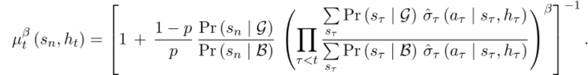
We here discuss the dynamics of beliefs and choices under an alternative model where players update beliefs in a non-Bayesian way.11 Player n of type β > 0 forms beliefs according to
µβt (sn, ht) = 1 + 1 − p p Pr (sn| G) Pr (sn| B) Y τ <t P sτ Pr (sτ | G) ˆστ(aτ | sτ, hτ) P sτ Pr (sτ | B) ˆστ(aτ | sτ, hτ) β −1 .
Players are Bayesian with β = 1, they underweight public relative to private information if β < 1, and overweight public relative to private information if β > 1. Types are drawn from a common distribution W . We assume that the distribution is commonly known such that assessed choice probabilities ˆστ(a | sτ, hτ) =
R∞
0 σ
β
τ(a | sτ, hτ) W (dβ) are correct averages across the distribution.
In period 1, all types follow private information. In later periods, behavior is characterized by a cutoff β∗(ht, qn) such that players of type β < β∗(ht, qn) follow private information of quality qn
at history ht whereas players of type β > β∗(ht, qn) contradict private information of quality qn at
ht. In particular, players with sufficiently small β < 1 follow private information even with the low
signal quality also at histories other than h1 = ∅ or ht= GBGB . . . GB. On the other hand, players
with sufficiently large β > 1 contradict private information even with the high signal quality at some histories. Since the cutoff is strictly increasing in the correctness of the signal, players respond to incentives but not perfectly so.
In general, whenever the (observed) population contains a sufficient mass of underweighters in-formation cascades start later, but each action conveys more inin-formation and beliefs become more extreme. Hence, even underweighters may eventually contradict private information with the high signal quality. In fact, non-Bayesian players may contradict private information less often than Bayes-rational players when endowed with a signal of low or medium quality and after short sequences of identical choices, and, at the same time, they may follow private information more often than Bayes-rational players when endowed with a high signal quality and after long sequences of identical choices.
3.3 Illustrations
Figure 1 and 2 plots the expected payoff of contradicting private information, mean pay|contradict, against the probability to contradict private information, prop contradict, in the level-k and
non-11
Bayesian equilibrium model, respectively.12 The expected payoff of contradicting private information is calculated under the assumption that observed adopt the Bayesian rational strategy (as they do in the Computer-Human treatment). Each marker reflects a distinct situation (sn, qn, ht) which occurs
with strictly positive probability. Green (blue, red) markers illustrate predictions for the medium (low, high) signal quality. Situations where the number of observed actions not favored by the signal minus the number of observed actions favored by the signal is strictly greater than 2 are highlighted with darker markers.
For both figures, the left panel corresponds to λ = 4 and the right panel corresponds to λ = 15. Figure 1 illustrates the predictions in the level-k model. The first, second, third and fourth row shows the predicted choice probabilities for L∞, L0, L1 and L2 players. Figure 2 illustrates the predictions
in the non-Bayesian equilibrium model. The first, second, third and fourth row shows the predicted choice probabilities for non-Bayesian players with β = 1/3, β = 2/3, β = 3/2, and β = 3.
Figure 1 shows that L∞ as well as L2 players with a sufficiently large λ respond appropriately
to the underlying incentives. In contrast, L0 players as well as L1 and L2 players with sufficiently
small λ suboptimally follow private information when endowed with a private signal of low or medium quality. Finally, L1 players na¨ıvely herd when endowed with a high quality signal as they contradict
private information if sufficiently many actions are observed which point in the opposite direction of their private signal.
Figure 2 shows that β < 1 players suboptimally follow private information with the low and me-dium signal quality. In contrast, β > 1 players suboptimally contradict private information with the high signal quality.
In summary, the level-k model and the non-Bayesian equilibrium model have the potential to predict a variety of regularities at the aggregate level. They may predict overweighting of private information with a low or a medium quality signal as well as na¨ıve herding with the high signal quality. Notice that only the non-Bayesian equilibrium model predicts the occurrence of both phenomena at the individual level assuming that sufficiently many players underweight public information (which is not the case in our illustration). Of course, the two behavioral models are fully specified only once the distribution of types is known. With the help of our large experimental dataset, we aim at reliably uncovering the type distributions of those two models.
4
Results
We first examine some aggregate properties of our data, and then we measure how successful parti-cipants are in learning from others.
4.1 Descriptive Statistics
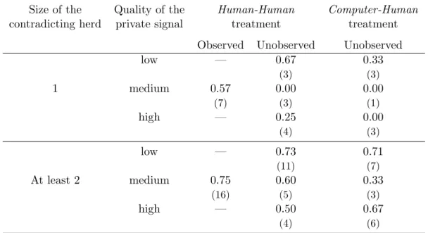
We start by presenting some summary statistics concerning the experimental choices in the first part of the experiment. Table 2 reports the proportion of herding choices when the size of the majority of previous choices against the private signal either equals one or is strictly greater than one. A majority of previous choices which point in the opposite direction of the private signal is called a contradicting herd. In line with the existing literature, observed give too much weight to their private information relative to the information conveyed by previous choices. Though the size of the contradicting herd
12For a given history h
t, when endowed with the realization of the private signal g and b the expected
pay-off of contradicting private information is given by mean pay|contradict (sn= g, ht) = Pr (B | sn= g, ht) and
ææ ææ ææ ææ ææ ææ æ æ æ æ ææ ææ ææææææ æ æ ææ L¥ 0 0.25 0.5 0.75 1 0 0.25 0.5 0.75 1 prop_contradict ææ æ æ æ æ æ æ æ æ ææ æ æ æ æ æ æ æ æ ææææææ æ ææ æ L¥ 0 0.25 0.5 0.75 1 0 0.25 0.5 0.75 1 æ æææ ææ ææææ æ æ æ æ æ æ æ æ æ æ ææææææ æ ææ æ L0 0 0.25 0.5 0.75 1 0 0.25 0.5 0.75 1 prop_contradict ææ ææ æ æ æ ææ æ æ æ æ æ æ æ æ æ æ æ ææææææ æ ææ æ L0 0 0.25 0.5 0.75 1 0 0.25 0.5 0.75 1 æææ æ æ æ ææ æ æ ææ ææ æ æ ææ æ æ æææææææ æ æ æ L1 0 0.25 0.5 0.75 1 0 0.25 0.5 0.75 1 prop_contradict ææ æ æ æ æ æ æ æ æ ææ æ æ æ æ æ æ æ æ ææææææ æ æ æ æ L1 0 0.25 0.5 0.75 1 0 0.25 0.5 0.75 1 ææææ æ æ æ æ æ æ ææ æ æ æ æ æ æ æ æ æææææææ æ æ æ L2 0 0.25 0.5 0.75 1 0 0.25 0.5 0.75 1 mean_payÈcontradict prop_contradict ææ æ æ æ æ æ æ æ æ ææ æ æ æ æ æ æ æ æ ææææææ æ ææ æ L2 0 0.25 0.5 0.75 1 0 0.25 0.5 0.75 1 mean_payÈcontradict
Figure 1: Predicted Probability to Contradict Private Information in the Level-k Model
ææææ æ æ æ æ æ æ ææ ææ æ æ æ æ æ æ ææææææ æ ææ æ Β = 1 3 0 0.25 0.5 0.75 1 0 0.25 0.5 0.75 1 prop_contradict ææ æ æ æ æ æ æ æ æ ææ æ æ æ æ æ æ æ æ ææææææ æ ææ æ Β = 1 3 0 0.25 0.5 0.75 1 0 0.25 0.5 0.75 1 ææ ææ æ æ æ æ æ æ ææ æ æ æ æ æ æ æ æ æææææææ ææ æ Β = 2 3 0 0.25 0.5 0.75 1 0 0.25 0.5 0.75 1 prop_contradict ææ æ æ æ æ æ æ æ æ ææ æ æ æ æ æ æ æ æ ææææææ æ ææ æ Β = 2 3 0 0.25 0.5 0.75 1 0 0.25 0.5 0.75 1 ææ ææ æ æ æ æ æ æ ææ æ æ æ æ æ æ ææ ææææææ æ æ æ æ Β = 3 2 0 0.25 0.5 0.75 1 0 0.25 0.5 0.75 1 prop_contradict ææ æ æ æ æ æ æ æ æ ææ æ æ æ æ æ ææ æ ææææææ æ æ æ æ Β = 3 2 0 0.25 0.5 0.75 1 0 0.25 0.5 0.75 1 ææ æ æ æ æ ææ ææ ææ æ æ æ æ æ ææ æ æææææ æ æ æ æ æ Β = 3 0 0.25 0.5 0.75 1 0 0.25 0.5 0.75 1 mean_payÈcontradict prop_contradict ææ æ æ æ æ æ ææ æ ææ æ æ æ æ æ ææ æ æææææ æ æ æ æ æ Β = 3 0 0.25 0.5 0.75 1 0 0.25 0.5 0.75 1 mean_payÈcontradict
Figure 2: Predicted Probability to Contradict Private Information in the Non-Bayesian Equilibrium Model
equals at least two, observed follow the herd in only 75 percent of the cases. When endowed with a private signal of medium quality, unobserved always herd less than observed (in both treatments). Even with a low quality signal unobserved never fully herd, and herding behavior is again comparable in both treatments. Still, the most surprising result is the large proportion of herding choices when unobserved are endowed with a high signal quality and they observe a contradicting herd of size at least two. In the latter cases, unobserved usually do not understand the value of the available information in the Computer-Human treatment.
Few experimental choices have been collected in the first part of the experiment since this part essentially served the purpose of letting participants gain experience with the social learning task (we collected 72 and 135 choices in the Computer-Human and Human-Human treatment, respect-ively). Moreover, a substantial proportion of choices seem to be the consequence of confusion. For example, observed contradict private information in about 13 percent of the cases where the majority of previous choices points either in no direction or in the same direction as the private signal. All remaining statistical analyzes rely exclusively on experimental choices made in the last three parts of the experiment.
Size of the Quality of the Human-Human Computer-Human
contradicting herd private signal treatment treatment
Observed Unobserved Unobserved
low — 0.67 0.33 (3) (3) 1 medium 0.57 0.00 0.00 (7) (3) (1) high — 0.25 0.00 (4) (3) low — 0.73 0.71 (11) (7) At least 2 medium 0.75 0.60 0.33 (16) (5) (3) high — 0.50 0.67 (4) (6)
Table 2: Proportion of Herding Choices in the First Part of the Experiment (number of observations in parentheses)
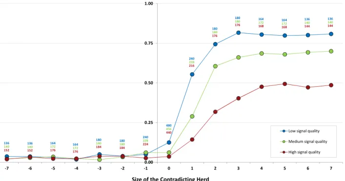
Figure 3 and 4 plots the size of the contradicting herd against the estimated probability of contra-dicting private information in the Computer-Human and Human-Human treatment, respectively.13 Probabilities have been obtained by estimating a logit regression model for each treatment and each role separately (Appendix 1 reports the regression results). The dependent variable is a dummy variable which takes value one if the choice contradicts private information and zero otherwise, and the explanatory variables are interaction effects between dummies for the sizes of the contradicting herd (from -7 to 7) and dummies for the signal qualities (we also included the dummy observed in the Human-Human treatment). The numbers of observations for each signal quality are shown on top of the regression lines.
Figure 3 confirms that unobserved when endowed with a private signal of low or medium quality fall prey to the ‘overweighting-of-private-information’ bias in the Computer-Human treatment. The
13
Note that contradicting herds of negative size are majorities of previous choices which point in the same direction as the private signal.
0.50 0.75 1.00 136 140 144 240 228 216 180 180 176 180 180 176 164 172 168 164 172 168 136 140 144 0.00 0.25 ‐7 ‐6 ‐5 ‐4 ‐3 ‐2 ‐1 0 1 2 3 4 5 6 7 Size of the Contradicting Herd Low signal quality Medium signal quality High signal quality 136 140 152 164 172 176 164 172 176 180 180 184 180 180 184 240 228 224 480 456 440 136 140 152
Figure 3: Estimated Probability to Contradict Private Information in the Computer-Human Treatment
0.50 0.75 1.00 77 73 79 ‐‐‐ 480 520 512 283 291 287 257 243 221 220 157 195 181 198 83 145 141 158 53 153 149 156 28 85 81 87 13 0.00 0.25 ‐7 ‐6 ‐5 ‐4 ‐3 ‐2 ‐1 0 1 2 3 4 5 6 7 Size of the Contradicting Herd Low signal quality Medium signal quality High signal quality Observed 75 79 73 ‐‐‐ 159 163 156 30 151 155 162 57 205 195 202 93 253 235 220 163 293 309 289 265 512 551 83 87 81 14
Figure 4: Estimated Probability to Contradict Private Information in the Human-Human Treatment
probability to contradict private information increases with the size of the contradicting herd until it reaches a plateau at about 0.8 for the low quality and 0.7 for the medium quality. Accordingly, unobserved do not sufficiently herd in situations where it is optimal to do so. Most remarkably, the tendency of unobserved to herd na¨ıvely when endowed with a private signal of high quality is also confirmed. As with lower signal qualities, the probability to contradict private information increases with the size of the contradicting herd, and it reaches one half. Though a contradicting herd of size
5 is not stronger evidence against private information than a contradicting herd of size 2, unobserved seem to believe that every imitative choice is informative to some extent.
Figure 4 shows that unobserved make similar choices in the Human-Human treatment than in the Computer-Human treatment, and that observed seem more willing to herd than unobserved who are endowed with the medium signal quality. Additionally, the comparison of the left half of the two figures suggests that unobserved doubt more the correctness of their private signal when the latter is confirmed by human choices than when it is confirmed by computer choices.
In summary, we observe the cascade phenomenon systematically reported in social learning exper-iments. Laboratory cascades occur among observed participants. Also in line with the existing literature, we find that observed are more willing to follow a contradicting herd the bigger the herd is. From the perspective of perfect Bayesian rationality, observed behave as if they discount the evidence conveyed by choices which are not part of an information cascade and they do not fully discount the evidence conveyed by cascade choices. The relative frequency with which they engage in cascade behavior equals the one usually reported in the literature, and this frequency is almost identical in the first part and the last three parts of the experiment (0.75 and 0.77 for contradicting herds of size at least 2, respectively). Thus, observed choices elicited under the direct-response and the (partial) strategy method are comparable.
Moreover, the qualitative behavior of observed and unobserved participants is similar when the latter are endowed with a weak or medium signal quality. However, unobserved with a medium signal quality exhibit an even stronger ‘overweighting-of-private-information’ bias than observed, and even more so in the Computer-Human treatment. This behavioral difference between the two groups of participants might result from the mistaken disposition of some unobserved to distinguish weak quality from medium quality choices when observing contradicting herds of size at least 2.
Finally, unobserved participants herd na¨ıvely when endowed with a high signal quality. In the Human-Human treatment, the majority of high quality choices disregard the private signal and follow others as soon as the contradicting herd reaches a size of 4.
4.2 The Success of Social Learning
Choice frequencies are reliable indicators of the success of social learning only in the Computer-Human treatment. And even in the latter treatment, it remains unknown how large are the parts of earnings that participants forgo when they rely too much on private signals of weak or medium quality or when they herd na¨ıvely with high signal quality. Building on Weizs¨acker (2010), we now measure how successful participants are in learning from others. To do so, we first assess the value of the available actions for unobserved participants which incidentally provides additional information on the behavior of observed participants. Once the value of actions is available, we determine the extent to which unobserved participants respond to the underlying incentives in situations where they should contradict weak or medium quality signals and in situations where they should follow the high quality signal.
4.2.1 The Value of Contradicting Private Information
In the Computer-Human treatment, the expected value of contradicting private information in period t when endowed with private signal snof quality qn∈ {12/21, 14/21, 18/21} and observing history ht
is given by
mean payCH|contradict(sn, qn, ht) =
1 +1−pp qn 1−qn Y τ <t qOσ∗(aτ|b,hτ)+(1−qO) σ∗(aτ|g,hτ) (1−qO) σ∗(aτ|b,hτ)+qOσ∗(aτ|g,hτ) −1 if sn= b 1 +1−pp qn 1−qn Y τ <t (1−qO) σ∗(aτ|b,hτ)+qOσ∗(aτ|g,hτ) qOσ∗(aτ|b,hτ)+(1−qO) σ∗(aτ|g,hτ) −1 if sn= g,
where σ∗ is the Bayesian rational strategy and qO= 14/21 is the signal quality of the observed players
(products in the above equation are assumed equal to one in the first period).
In the Human-Human treatment, we rely on a modified version of Weizs¨acker’s (2010) counting technique to estimate the expected value of contradicting private information.14 Accordingly,
mean payHH|contradict(sn, qn, ht) =
1 +1−pp qn 1−qn Y τ <t qOP r(aˆ τ|b,hτ,B)+(1−qO) ˆP r(aτ|g,hτ,B) (1−qO) ˆP r(aτ|b,hτ,G)+qOP r(aˆ τ|g,hτ,G) −1 if sn= b 1 +1−pp qn 1−qn Y τ <t (1−qO) ˆP r(aτ|b,hτ,G)+qOP r(aˆ τ|g,hτ,G) qOP r(aˆ τ|b,hτ,B)+(1−qO) ˆP r(aτ|g,hτ,B) −1 if sn= g,
where ˆP r (aτ | sn, hτ, ω) is the relative frequency with which action aτ is chosen across all observed
choices where the private signal is sn, the history is hτ and the state of Nature is ω ∈ {B, G}
(products in the above equation are assumed equal to one in the first period). The empirical value of contradicting private information in the Human-Human treatment is a consistent estimate of the true expected value of contradicting private information whatever the behavioral model of observed players. Still, the precision with which mean payHH|contradict(sn, qn, ht) estimates the underlying expected
value depends on the number of observations with identical (sn, qn, ht). When few observations are
available, the estimate might be far from its expected value. But relying only on situations (sn, qn, ht)
with many observations implies that relatively few values of mean payHH|contradict(sn, qn, ht) are
available. Unless otherwise specified, statistical analyzes which use the expected value of contradicting private information in the Human-Human treatment exclude situations which appear in two or less distinct repetitions of the social learning game (for a total of 36 repetitions).15
We now compare the incentives to contradict private information for the unobserved participants in the two treatments. Table 3 summarizes the distribution of the empirical value of contradicting private information for each signal quality, simply denoted by mpc, in each treatment. The two dis-tributions are largely comparable for each signal quality which confirms that the behavior of observed participants is reasonably close to the behavior of (almost) Bayes-rational players. As expected, the incentives to follow private information with a high signal quality are quite substantial and more so in the Computer-Human treatment. In contrast, when endowed with a low or medium signal quality unobserved should contradict private information in some situations.
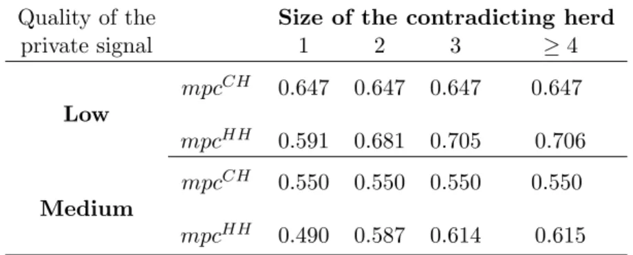
To better appreciate the benefits associated with contradicting low or medium quality private information when observed choices point in the opposite direction, Table 4 reports the median values of mpc as a function of the size of contradicting herds. Contrary to the Computer-Human treatment, incentives to follow others increase with the size of the contradicting herd in the Human-Human treatment, until the herd size equals 4. This observation confirms that observed participants do
14See Ziegelmeyer, March, and Kruegel (2011) for details. 15
The qualitative insights of our data analyzes do not change when the requirement on the precision of the estimate is strengthened. The results of those robustness checks are available from the authors upon request.
Quality of the Percentile private signal 1% 5% 10% 25% 50% 75% 90% 95% 99% mpcCH 0.186 0.186 0.235 0.235 0.380 0.647 0.711 0.711 0.711 Low mpcHH 0.183 0.183 0.190 0.209 0.424 0.681 0.706 0.715 0.715 mpcCH 0.133 0.133 0.170 0.170 0.379 0.550 0.550 0.621 0.621 Medium mpcHH 0.116 0.130 0.135 0.149 0.318 0.526 0.615 0.626 0.657 mpcCH 0.048 0.048 0.064 0.064 0.120 0.289 0.289 0.353 0.353 High mpcHH 0.042 0.047 0.050 0.070 0.145 0.322 0.347 0.358 0.389
Table 3: Empirical Value of Contradicting Private Information in Each Treatment
not systematically engage in cascade behavior after few contradicting choices but almost always do so after many contradicting choices. For contradicting herds larger than two, incentives advise to contradict private information. However, the expected gain from contradicting medium quality private information is small which indicates that low quality choices are more appropriate to identify the ‘overweighting-of-private-information’ bias.
Quality of the Size of the contradicting herd
private signal 1 2 3 ≥ 4 mpcCH 0.647 0.647 0.647 0.647 Low mpcHH 0.591 0.681 0.705 0.706 mpcCH 0.550 0.550 0.550 0.550 Medium mpcHH 0.490 0.587 0.614 0.615
Table 4: Median Empirical Value of Contradicting Private Information and Size of the Contradicting Herd in Each Treatment
4.2.2 Overweighting of Private Information and Na¨ıve Herding
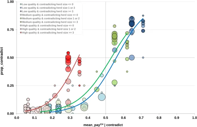
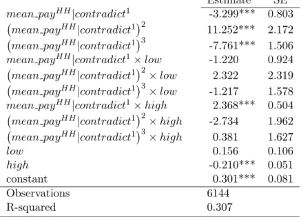
Figure 5 and 6 plots the empirical value of contradicting private information against the proportion of choices which contradict private information in the Computer-Human and Human-Human treat-ment, respectively. For each situation (restricted to situations which appear in at least three distinct repetitions of the game in the Human-Human treatment), the figures contain a bubble with x-value the empirical value of contradicting private information and y-value the proportion of choices which contradict private information, and the bubble’s size reflects the number of observations. Each figure also includes a regression line for each signal quality (details about the regressions are to be found in Appendix 2).16
16
Only choices made in the fourth part of the experiment are included. Regression analyzes show an absence of significant behavioral change in the course of the experiment. Details are available from the authors upon request.
0.50 0.75 1.00 p rop _ co ntradict
Low quality & contradicting herd size <= 0 Low quality & contradicting herd size 1 or 2 Low quality & contradicting herd size >= 3 Medium quality & contradicting herd size <= 0 Medium quality & contradicting herd size 1 or 2 Medium quality & contradicting herd size >= 3 High quality & contradicting herd size <= 0 High quality & contradicting herd size 1 or 2 High quality & contradicting herd size >= 3
0.00 0.25
0.0 0.1 0.2 0.3 0.4 0.5 0.6 0.7 0.8 0.9 1.0
p
mean_payCH| contradict
Figure 5: Proportion of Choices which Contradict Private Information in the Computer-Human Treatment
0.50 0.75 1.00 p rop _ co ntradict
Low quality & contradicting herd size <= 0 Low quality & contradicting herd size 1 or 2 Low quality & contradicting herd size >= 3 Medium quality & contradicting herd size <= 0 Medium quality & contradicting herd size 1 or 2 Medium quality & contradicting herd size >= 3 High quality & contradicting herd size <= 0 High quality & contradicting herd size 1 or 2 High quality & contradicting herd size >= 3
0.00 0.25
0.0 0.1 0.2 0.3 0.4 0.5 0.6 0.7 0.8 0.9 1.0
p
mean_payHH| contradict
Figure 6: Proportion of Choices which Contradict Private Information in the Human-Human Treatment
When endowed with a private signal of low or medium quality, unobserved participants respond reasonably well to the underlying incentives in each treatment.
In the Human-Human treatment, the average participant follows private information only in situations where it is optimal to do so. Both the blue and green regression lines are basically S-shaped lines through (0.5, 0.5). We can never reject the hypothesis that participants exhibit a correct perception of the value of contradicting private information since the vertical distance between the regression line and (0.5, 0.5) is not significant (p-value equals 0.348 and 0.914 with low and medium quality). Moreover, participants use their information with identical success in situations where they should follow others than in situations where they should follow their private signal. In situations where the empirical value of contradicting private information is strictly larger than 0.5, the relative frequency of optimal choice is 0.794 and 0.703 with a low and medium signal quality, respectively. In situations with similar incentives but where the empirical value of contradicting private information is strictly smaller than 0.5, the relative frequency of optimal choice is 0.776 and 0.713 with a low and medium signal quality, respectively.17
In the Computer-Human treatment, participants follow others with more than probability 0.5 in situations where the empirical value of contradicting private information is larger than 0.560 and 0.532 with a low and medium signal quality, respectively. The vertical distance between the regression line and (0.5, 0.5) is significantly different from zero with a low signal quality (p-value equals 0.002) which confirms the existence of the ‘overweighting-of-private-information’ bias. However, we cannot reject the hypothesis that participants exhibit a correct perception of the value of contradicting private information with medium quality (p-value equals 0.208). The slight tendency of participants to mistakenly discount the evidence conveyed by the predictions of computers is confirmed by their relative success of learning from others. In situations where the empirical value of contradicting private information is strictly larger than 0.5, the relative frequency of optimal choice is 0.755 and 0.607 with a low and medium signal quality, respectively. In situations with similar incentives but where the empirical value of contradicting private information is strictly smaller than 0.5, the relative frequency of optimal choice is 0.888 and 0.879 with a low and medium signal quality, respectively.18 To our surprise, participants are less successful in following computer than human choices in situations where it is empirically optimal to do so.
The fact that participants assess the expected value of actions only imperfectly is confirmed by a series of regression analyzes. These analyzes control for the value of contradicting private information to determine whether non payoff-relevant aspects of the situation influence participants’ behavior. We find that, when endowed with a private signal of low or medium quality, unobserved contradict private information to a larger extent the bigger the size of the contradicting herd though the empir-ical value of contradicting private information is kept constant (details are available from the authors upon request). In conclusion, participants mistakenly adopt a sort of counting rule as they do not discount sufficiently the evidence conveyed by late cascade choices.
17In situations where they should follow others, the range of the empirical value of contradicting private information
is ]0.500, 0.715] and ]0.500, 0.657] with a low and medium signal quality, respectively (see Table 3). Thus, the mirrored range below 0.5 which corresponds to situations with relatively weak incentives to follow private information is [0.285, 0.500[ and [0.343, 0.500[ with a low and medium signal quality, respectively. In all situations where the empirical value of contradicting private information is below 0.5, the relative frequency of optimal choice is 0.862 and 0.874 with a low and medium signal quality, respectively.
18
In situations where they should follow others, the range of the empirical value of contradicting private information is ]0.500, 0.711] and ]0.500, 0.621] with a low and medium signal quality, respectively (see Table 3). Thus, the mirrored range below 0.5 which corresponds to situations with relatively weak incentives to follow private information is [0.289, 0.500[ and [0.379, 0.500[ with a low and medium signal quality, respectively. In all situations where the empirical value of contradicting private information is below 0.5, the relative frequency of optimal choice is 0.943 and 0.949 with a low and medium signal quality, respectively.
In contrast, when endowed with a private signal of high quality, unobserved participants respond rather badly to the underlying incentives in each treatment. Both figures show that once the size of the contradicting herd is big enough the average participant follows others though incentives clearly advise to follow private information. Our analysis of the social learning success establishes that participants forgo large parts of their earnings when herding na¨ıvely. Indeed, in each treatment, unobserved herd na¨ıvely on average in situations where the empirical value of contradicting private information approximately equals 1/3: In such situations, the evidence conveyed by the observable choices is so weak that the private information is correct more than twice as often as it is wrong. In situations with identical incentives but in the absence of big contradicting herds, participants largely follow private information whatever the quality of the private signal.
5
Conclusion
Since the seminal paper of Anderson and Holt (1997), the economic literature on experimental social learning games investigates whether participants are capable of making rational inferences in con-trolled settings. Notwithstanding the tendency to overweight private information relative to public information, the literature concluded that participants generally use their information efficiently and follow others only in warranted situations.
Our results severely undermine the robustness of this conclusion. We show that participants forgo large parts of earnings by following others in situations where they should contradict them. Our new evidence therefore suggests that participants are prone to a ‘social-confirmation’ bias and it gives support to the argument that they na¨ıvely believe that each observable choice reveals a substantial amount of that person’s private information. At the aggregate level, participants’ behavior seems best describe by a counting rule which discounts the early cascade choices and does not fully discount the late cascade choices.
Thanks to the large amount of data collected at the individual level, we have classified the social learning behavior of each of our unobserved participants. Though a substantial fraction of parti-cipants (almost) always follow their private information, we also find a substantial fraction of social-conformists who follow contradicting herds of any size (details are available from the authors upon request). Clearly, some unobserved participants drew opposite conclusions from the same evidence. Further experimental work on social learning should dig deeper into this heterogeneity in informational inferences.
Appendix 1: Regression Results for Figure 3 and 4
Human-Human treatment Computer-Human treatment
Observed Unobserved Unobserved
Estimate SE Estimate SE Estimate SE
Low Quality × Size = −7 — — -2.876*** 0.500 -3.266*** 0.671 Size = −6 — — -3.283*** 0.579 -3.266*** 0.671 Size = −5 — — -2.419*** 0.351 -3.459*** 0.505 Size = −4 — — -2.281*** 0.368 -3.983*** 0.557 Size = −3 — — -2.469*** 0.444 -2.944*** 0.526 Size = −2 — — -1.897*** 0.319 -3.207*** 0.626 Size = −1 — — -1.934*** 0.325 -2.944*** 0.418 Size = 0 — — -1.132*** 0.226 -1.946*** 0.266 Size = 1 — — 0.683*** 0.191 0.218 0.283 Size = 2 — — 1.229*** 0.312 1.069*** 0.345 Size = 3 — — 1.628*** 0.356 1.494*** 0.378 Size = 4 — — 1.776*** 0.371 1.417*** 0.408 Size = 5 — — 1.784*** 0.358 1.379*** 0.407 Size = 6 — — 1.906*** 0.474 1.396*** 0.404 Size = 7 — — 2.022*** 0.533 1.442*** 0.449 Medium Quality × Size = −7 — — -3.651*** 0.718 -3.821*** 0.750 Size = −6 (omitted) — -3.332*** 0.597 -3.526*** 0.618 Size = −5 (omitted) — -2.626*** 0.384 -3.320*** 0.570 Size = −4 -4.025*** 1.061 -2.786*** 0.451 -3.738*** 0.603 Size = −3 -3.818*** 1.032 -2.725*** 0.479 -4.078*** 0.746 Size = −2 -3.264*** 0.521 -2.321*** 0.354 -3.367*** 0.512 Size = −1 -2.402*** 0.330 -1.995*** 0.314 -2.727*** 0.558 Size = 0 -1.895*** 0.338 -1.605*** 0.295 -2.727*** 0.435 Size = 1 -0.849*** 0.208 -0.587*** 0.189 -0.898*** 0.215 Size = 2 0.912*** 0.264 0.470** 0.225 0.429 0.333 Size = 3 1.432*** 0.450 1.077*** 0.344 0.668 0.362 Size = 4 1.587** 0.628 0.926*** 0.348 0.782** 0.355 Size = 5 1.526** 0.669 1.144*** 0.384 0.755** 0.378 Size = 6 1.705** 0.809 1.183*** 0.422 0.814** 0.400 Size = 7 — — 1.192*** 0.429 0.847** 0.389 High Quality × Size = −7 — — -3.150*** 0.730 -3.905*** 0.573 Size = −6 — — -2.721*** 0.486 -3.381*** 0.678 Size = −5 — — -2.579*** 0.439 -3.761*** 0.600 Size = −4 — — -2.526*** 0.430 -3.761*** 0.600 Size = −3 — — -2.677*** 0.432 -3.230*** 0.542 Size = −2 — — -2.303*** 0.401 -3.230*** 0.658 Size = −1 — — -2.193*** 0.380 -3.593*** 0.700 Size = 0 — — -2.038*** 0.393 -3.277*** 0.557 Size = 1 — — -1.395*** 0.308 -1.786*** 0.383 Size = 2 — — -0.659** 0.300 -0.762*** 0.293 Size = 3 — — -0.162 0.293 -0.391 0.314 Size = 4 — — 0.076 0.318 -0.095 0.311 Size = 5 — — 0.154 0.331 -0.024 0.320 Size = 6 — — 0.023 0.353 -0.111 0.337 Size = 7 — — 0.178 0.365 -0.056 0.328 Observations 1720 8640 8640 Log pseudo-likelihood -664.32 -3742.56 -3041.86
Notes: Robust standard errors clustered at the individual level. Two variables were omitted from the regression for the observed since the latter always followed private information.