Volatility Models : from GARCH to Multi-Horizon Cascades

HAL Id: halshs-00390636

https://halshs.archives-ouvertes.fr/halshs-00390636

Submitted on 2 Jun 2009

HAL is a multi-disciplinary open access

archive for the deposit and dissemination of

sci-L’archive ouverte pluridisciplinaire HAL, est

destinée au dépôt et à la diffusion de documents

Volatility Models : from GARCH to Multi-Horizon

Cascades

Alexander Subbotin, Thierry Chauveau, Kateryna Shapovalova

To cite this version:

Alexander Subbotin, Thierry Chauveau, Kateryna Shapovalova. Volatility Models : from GARCH to

Multi-Horizon Cascades. 2009. �halshs-00390636�

Documents de Travail du

Centre d’Economie de la Sorbonne

Volatility Models : from GARCH to Multi-Horizon Cascades

A

S

T

C

K

S

Volatility Models:

from GARCH to Multi-Horizon Cascades

∗

Alexander Subbotin

_{Thierry Chauveau}

Kateryna Shapovalova

May 15, 2009

∗_{The authors thank Patrick Artus for help and encouragement in preparing this work. The} usual disclaimers apply.

†_{University of Paris-1 (Panth`eon-Sorbonne) and Higher School of Economics. E-mail:} alexander.subbotin@univ-paris1.fr

Abstract

We overview different methods of modeling volatility of stock prices and exchange rates, focusing on their ability to reproduce the empirical properties in the corresponding time series. The properties of price fluctu-ations vary across the time scales of observation. The adequacy of different models for describing price dynamics at several time horizons simultane-ously is the central topic of this study. We propose a detailed survey of recent volatility models, accounting for multiple horizons. These mod-els are based on different and sometimes competing theoretical concepts. They belong either to GARCH or stochastic volatility model families and often borrow methodological tools from statistical physics. We compare their properties and comment on their practical usefulness and perspec-tives.

Keywords: Volatility modeling, GARCH, stochastic volatility, volatil-ity cascade, multiple horizons in volatilvolatil-ity.

J.E.L. Classification: G10, C13.

R´esum´e

Nous pr´esentons diff´erentes m´ethodes de mod´elisation de la volatilit´e des prix des actions et des taux de change en prˆetant une attention particuli`ere `a leur capacit´e `a reproduire les pro-pri´et´es empiriques des s´eries temporelles. Nous montrons que l’´echelle de temps d’observation a une influence sur les propri´et´es des variations des prix. Le th`eme de cette ´etude est de discuter de la capacit´e des mod`eles de volatilit´e `a d´ecrire simultan´ement la dynamique des prix `a plusieurs ´echelles de temps. Nous effec-tuons une analyse d´etaill´ee des mod`eles de volatilit´e r´ecents qui tiennent compte d’horizons multiples. Ces mod`eles sont fond´es sur des concepts th´eoriques diff´erents et quelquefois en concur-rence. Ils appartiennent `a des familles de mod`eles GARCH ou volatilit´e stochastique, les deux groupes empruntant souvent des outils m´ethodologiques de la physique statistique. Nous com-parons leurs propri´et´es et concluons sur leur utilit´e pratique et les perspectives d’utilisation qu’ils ouvrent.

Mots cl´es: mod´elisation de la volatilit´e, GARCH, volatilit´e stochastique, cascade de volatilit´e, horizons multiples dans la volatilit´e.

1

Introduction

Modeling stock prices is essential in many areas of financial economics, such as derivatives pricing, portfolio management and financial risk follow-up. One of the most criticized drawbacks of the so-called “modern portfolio theory” (MPT), including the diversification principle of Markowitz (1952) and the cap-ital asset pricing model by Sharpe (1964) and Lintner (1965), is the non-realistic assumption about stock price variability. Clearly, stock returns are not iid dis-tributed Gaussian random variables, but alternatives to this assumption are numerous, sometimes complicated and application-dependent. In this paper we review empirical properties of stock price dynamics and various models, pro-posed to represent it, focusing on the most recent developments, concerning mainly multi-horizon and multifractal stochastic volatility processes.

The subject of this study is the variability of stock prices, referred to as volatility. Usually introduction of scientific terminology aims at making a gen-eral concept more precise, but this is rather an example of the contrary. De-pending on the context and the point of view of the author, the term “volatility” in finance can stand for the variability of prices (in this sense we used it above), an estimate of standard deviation, financial risk in general, a parameter of a derivative pricing model or a stochastic process of particular form. We will continue using it in the most general sense, that is as a synonym of variability. Before reviewing volatility models, we examine in more detail the evolution of the notion itself. This will help for a better understanding of the logic of the evolution of the corresponding models.

One of the first interpretations of the term “volatility” is due to the fact that the name of variability phenomenon itself has been identified with the most elementary method of its quantitative measurement - standard deviation of stock returns. This interpretation is logically embedded in the concept of MPT, also called mean-variance theory, because under its assumptions these two parameters contain all relevant information about stock returns, distributed normally1_{. Note that in Markowitz (1952) risk is modeled statically: returns}

on each stock are characterized by constant volatility (variance or standard deviation) and covariances with the returns on other assets. So volatility can be seen as synonym for standard deviation, or as an estimate of a constant parameter in the simplest model of stock returns. This definition of volatility has deep roots and is still widely used among asset management professionals.

The appearance in 1973 of the option pricing models by Black and Scholes (1973) and Merton (1973) led to significant changes in the understanding of volatility. A continuous-time diffusion (geometric Brownian motion) is used to model stock prices:

dSt

St

= µdt + σdWt (1)

with Stthe stock price, µ the drift parameter and Wta Brownian motion. The

parameter σ is called volatility because it characterizes the degree of variability. Since the log-returns, computed from stock prices that follow equation (1), are normally distributed, this model is also called a log-normal diffusion.

Very soon it became obvious that equation (1) poorly describes reality. Its parameters unambiguously define option prices for given exercise dates and

strikes, so that volatility parameter can be inferred from observations of option prices by using the inverse of the Black-Scholes formula. An estimate obtained in this way is called implied volatility as opposed to historical volatility, mea-sured as the standard deviation of returns. Contrary to the predictions of the Black and Scholes model empirical results show that implied volatility varies for option contracts with different parameters. This phenomenon is known as volatility smile. Its name is due to a characteristic convex form of the plot of the estimate of σ as function of the option exercise price.

The above remark does not mean that implied volatility is useless. It has been shown that it contains information about future variability of returns and thus it is often used in forecasting. In derivatives pricing implied volatility is important because it allows to extrapolate the observed market data, e.g. option prices, for the evaluation of other financial instruments, e.g. over-the-counter options (see Dupire, 1993, 1994; Avellaneda et al., 1997). Despite these partial successes, a more adequate model than log-normal diffusion could still be useful in both derivatives pricing and asset management applications. In Merton (1973) volatility parameter is already allowed to vary in time. Even earlier Mandelbrot (1963) points to the empirical properties of stock returns that to not correspond to the log-normal diffusion model and proposes a wider class of Levy-stable probability distributions. Further developments in the led to the understanding of volatility as a stochastic process and not merely as a parameter, even time-varying.

The meaning of the term “volatility” in finance has come full circle: from a general term for variability phenomenon to a statistical estimate, then a model parameter and finally a stochastic process, which again is supposed to charac-terize the whole structure of the stock price variability. More technically, the modern understanding of volatility can be characterized as a time structure of conditional second-order moments in the distribution of returns. In the simplest case of log-normal diffusion this structure is described by one parameter and in more complicated cases, by a separate stochastic process.

This paper starts with an overview of empirical properties of volatility, the so-called “stylized facts”. Then we briefly discuss traditional approaches to its modeling - conditional heteroscedasticity and stochastic volatility, that re-produce empirical properties to some extent. Though many models are good enough to describe separate stylized facts, we show that none of them is quite sufficient to represent the whole structure of stock price variability. In particu-lar, most traditional models do not allow for representing returns dynamics on multiple time horizons (e.g. from minutes to days and months) simultaneously, which is important both practically and theoretically. Stylized facts themselves have features specific to the frequency, at which price dynamics is observed. We analyze and compare recently proposed models of conditional heteroscedasticity and stochastic volatility, based on the multi-horizon approach, and discuss the main unsolved problems, related to them.

detailed survey on the subject see Cont (2001).

• Excessive volatility. The observed degree of variability in stock prices can hardly be explained by variations in fundamental economic factors. In particular, returns of large magnitude (positive and negative) are often hard to explain by arrival of new information about future cash flows (Cutler et al., 1989).

• Absence of linear correlations in returns. Stock returns, computed over sufficiently long time periods (several hours and more) display in-significant linear correlation. This results is in accordance with the stock market efficiency hypothesis by Fama (1970) and the main results of MPT, using martingale measures.

• Clustering of volatility and long memory in absolute values of returns. Time series of absolute values of returns is characterized by important autocorrelation, and the autocorrelation function (ACF) decays slowly with time lags (slower than geometric decay). Long periods of high and low volatility are observed (Bollerslev et al., 1992; Ding et al., 1993; Ding and Granger, 1996).

• The link between the trading volume and volatility. Volatility of returns is positively correlated with the trading volume, and the latter time series displays the same long memory properties as in the absolute returns (Lobato and Velasco, 2000).

• Asymmetry and leverage in the dynamic structure of volatil-ity. Positive and negative returns of the same magnitude, observed over the past period, have different effects on current volatility (asymmetry). Current returns and future volatility are negatively correlated (leverage). Presence of the leverage effect implies the asymmetry but the inverse does not hold (Black, 1976).

• Heavy tails in the distribution of returns. Unconditional probability distribution of daily returns is characterized by heavy tails, i.e. high prob-ability of observing extreme values, compared to the normal distribution (Mandelbrot, 1963; Fama, 1965).

• The form of the probability distribution of returns varies across time intervals, over which returns are computed(Ghashghaie et al., 1996; Arneodo et al., 1998). Distributions of log-returns over long time intervals are relatively close to the normal law, while returns over short time intervals (5 - 30 minutes) have very heavy tails.

Among these stylized facts we shall be particularly interested in the proper-ties related to the ACF of returns and the form of the probability distribution of returns and their magnitudes. We start with a definition of the above-mentioned long memory phenomenon in terms of ACF.

A stationary stochastic process Xtwith finite variance has long memory (or

long-range dependence) if its autocorrelation function C(τ ) = corr(Xt, Xt−τ) at

τ → ∞ decays with the time lag according to the power low (i.e. at hyperbolic speed):

where 0 < d < 1₂ and where L(·) is some continuous function that for ∀x > 0 and τ → ∞ satisfies L(xt)L(t) → 1. The process has short memory if its ACF decays

exponentially (with geometric speed), so that:

∃A > 0, c ∈ (0, 1) : |C(τ)| ≤ Acτ (3)

In this definition the technical condition, imposed on the function L(·), im-plies that for infinite lag τ this function changes infinitely slowly. Notice that the definition refers to the theoretical ACF of the time series model and not to its sample estimate. As we will see, in many cases the sample ACF has prop-erties, similar to those implied by definition (2), but the theoretical ACF does not satisfy this definition.

Alternatively, long memory can be characterized by the power law divergence of the spectral density of the time series Xtat the origin:

Ψx(u) ∼ cΨ|u|−α (4)

with Ψx(·) - spectral density function, α - scaling parameter and cΨ- a constant.

To illustrate the empirical properties of returns we use two types of stock index data: high frequency (intraday) observations over a relatively short time period (French CAC40 index) and daily observations for very long time pe-riod (Dow Jones Industrial Average Index, DJIA). We will see that the main empirical patterns are similar for these very different examples.

The return at time t ∈ 1 . . . T over the interval τ is defined as the change in the logarithm of price S:

rt= ln(St) − ln(St−τ). (5)

As a measure of volatility we take the magnitude of return |rt|. Note that

similar results could be obtained for squared returns and, most generally, for |rt|α (Bollerslev et al., 1992; Ding et al., 1993; Ding and Granger, 1996), but

for α = 1 the long memory properties are more pronounced (Ding et al., 1993; Ghysels et al., 2006; Forsberg and Ghysels, 2007).

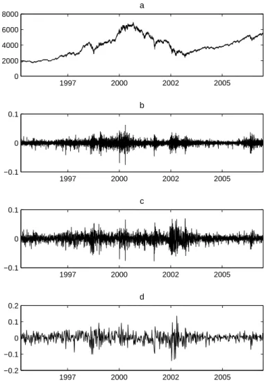
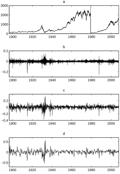
Figures 1 and 2 represent the time series of index values and returns, com-puted over different time intervals. For the CAC40 index we compute 15-minutes, daily and weekly returns, and for the DJIA index - daily, monthly and quarterly returns. On both data sets the phenomenon of volatility cluster-ing can be easily identified: long-lastcluster-ing and persistent periods of returns with high magnitude (positive and negative) alternate with low volatility periods. High volatility is rarely observed on up-going market trend. Large fluctuations are characteristic of trend reversals and slumps.

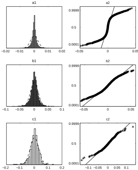
Now consider the form of the probability distribution of returns, computed over different time intervals (Figures 3 and 4). For 15-minutes returns on the CAC40 index the distribution is clearly leptokurtic: the deviation from the nor-mal curve in the tails is significant. As the frequency of observations is reduced this deviation decreases. This can be interpreted as an effect of the central limit theorem, though the the adequacy of hypotheses underlying its various forms is

Figure 1: Returns on the CAC40 Index 1997 2000 2002 2005 0 2000 4000 6000 8000 a 1997 2000 2002 2005 −0.1 0 0.1 b 1997 2000 2002 2005 −0.1 0 0.1 c 1997 2000 2002 2005 −0.2 −0.1 0 0.1 0.2 d

Source: Euronext, CAC40 index from 20/03/1995 to 29/12/2006 at 15-minutes intervals, 100881 observations. the figure shows a: index values; b: 15-minute returns, 100880 observa-tions; c: daily returns, 2953 observaobserva-tions; d: weekly returns, 590 observations.

Figure 2: Returns on the DJIA Index 1900 1920 1940 1960 1980 2000 0 1000 2000 3000 a 1900 1920 1940 1960 1980 2000 −0.2 0 0.2 b 1900 1920 1940 1960 1980 2000 −0.4 −0.2 0 0.2 c 1900 1920 1940 1960 1980 2000 −0.5 0 0.5 d

Source: Dow Jones Indexes, daily values of the DJIA index from 26/05/1896 to 10/10/2007, 28864 observations. The figure shows a: index values (for visualization purposes the values of index are reset to 100 at the beginning of the period and then again at 01/01/1979); b: daily returns, 28863 observations; c: monthly returns, 2953 observations; d: quarterly returns, 444 observations.

Figure 3: Probability Distribution of Returns on the CAC40 Index −0.02 −0.01 0 0.01 0.02 a1 −0.05 0 0.05 0.0001 0.5 0.9999 a2 −0.1 −0.05 0 0.05 0.1 b1 −0.05 0 0.05 0.0001 0.5 0.9999 b2 −0.2 −0.1 0 0.1 0.2 c1 −0.1 −0.05 0 0.05 0.1 0.0001 0.5 0.9999 c2

Source: Euronext, values of index CAC40 from 20/03/1995 to 29/12/2006 at 15-minutes intervals, 100881 observations. The figure shows a1: histogram of the distribution density and its log-normal approximation for 15-minutes returns, 100880 observations; a2: probability plot for the same data, i.e. empirical cumulative distribution function (cdf), compared with the theoretical normal cdf (if the normal distribution perfectly approximates the empirical distribution, all points are on the diagonal straight line); b1,2: the same for daily returns, 2953 observations; c1,2: the same for weekly returns, 590 observations.

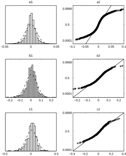
Figure 4: Probability Distribution of Returns on the DJIA Index −0.05 0 0.05 a1 −0.1 −0.05 0 0.05 0.1 0.0001 0.5 0.9999 a2 −0.2 −0.1 0 0.1 0.2 b1 −0.2 −0.1 0 0.1 0.2 0.0001 0.5 0.9999 b2 −0.5 0 0.5 c1 −0.4 −0.2 0 0.2 0.4 0.0001 0.5 0.9999 c2

Source: Dow Jones Indexes, daily values of the DJIA index from 26/05/1896 to 10/10/2007, 28864 observations. The figure shows a1: histogram of the distribution density and its log-normal approximation for daily returns, 28863 observations; a2: probability plot for the same data, i.e. empirical cumulative distribution function (cdf), compared with the theoretical normal cdf (if the normal distribution perfectly approximates the empirical distribution, all points are on the diagonal straight line); b1,2: the same for monthly returns, 2953 observations; c1,2: the same for quarterly returns, 590 observations.

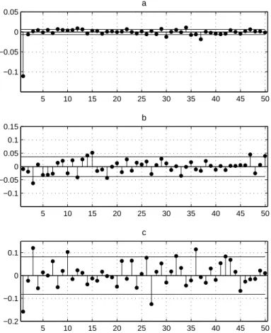
Figure 5: Sample ACF for the Returns on the CAC40 Index 5 10 15 20 25 30 35 40 45 50 −0.1 −0.05 0 0.05 a 5 10 15 20 25 30 35 40 45 50 −0.1 −0.05 0 0.05 0.1 0.15 b 5 10 15 20 25 30 35 40 45 50 −0.2 −0.1 0 0.1 c

Source: Euronext, values of index CAC40 from 20/03/1995 to 29/12/2006 at 15-minutes intervals, 100881 observations. The figure shows a: ACF for 15-minutes returns, 100880 ob-servations; b: the same for daily returns ,2953 obob-servations; c: the same for weekly returns, 590 observations. Horizontal solid lines show confidence intervals for autocorrelations, computed under assumption that returns are normal white noise.

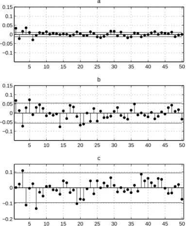
Figure 6: Sample ACF for the Returns on the DJIA Index 5 10 15 20 25 30 35 40 45 50 −0.1 −0.05 0 0.05 0.1 0.15 a 5 10 15 20 25 30 35 40 45 50 −0.1 −0.05 0 0.05 0.1 0.15 b 5 10 15 20 25 30 35 40 45 50 −0.2 −0.1 0 0.1 c

Source: Dow Jones Indexes, daily values of the DJIA index from 26/05/1896 to 10/10/2007, 28864 observations. The figure shows a: ACF for daily returns, 28863 observations; b: the same for daily returns ,2953 observations; c: the same for quarterly returns, 590 observa-tions. Horizontal solid lines show confidence intervals for autocorrelations, computed under assumption that returns are normal white noise.

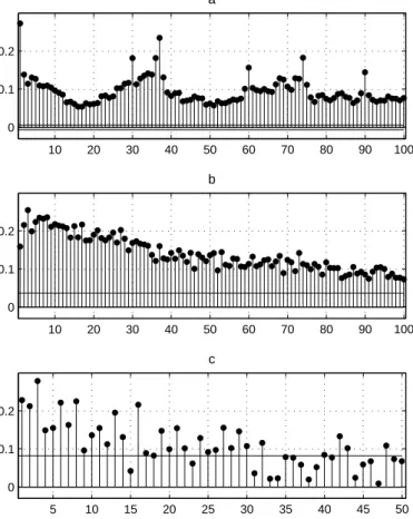
Figure 7: Sample ACF for the Magnitudes of Returns on the CAC 40 Index 10 20 30 40 50 60 70 80 90 100 0 0.1 0.2 a 10 20 30 40 50 60 70 80 90 100 0 0.1 0.2 b 5 10 15 20 25 30 35 40 45 50 0 0.1 0.2 c

Source: Euronext, values of index CAC40 from 20/03/1995 to 29/12/2006 at 15-minutes intervals, 100881 observations. The same as on Figure 5, but instead of returns their absolute values are used.

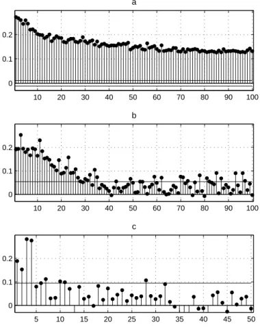
Figure 8: Sample ACF for the Magnitudes of Returns on the DJIA Index 10 20 30 40 50 60 70 80 90 100 0 0.1 0.2 a 10 20 30 40 50 60 70 80 90 100 0 0.1 0.2 b 5 10 15 20 25 30 35 40 45 50 0 0.1 0.2 c

Source: Dow Jones Indexes, daily values of the DJIA index from 26/05/1896 to 10/10/2007, 28864 observations. The same as on Figure 6, but instead of returns their absolute values are used.

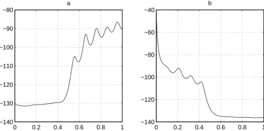
Figure 9: Sample Spectrum Density Function for the Returns on the CAC40 Index and their Magnitudes

0 0.2 0.4 0.6 0.8 1 −140 −130 −120 −110 −100 −90 −80 a 0 0.2 0.4 0.6 0.8 1 −140 −120 −100 −80 −60 −40 b

Source: Euronext, values of index CAC40 from 20/03/1995 to 29/12/2006 at 15-minutes intervals, 100881 observations. the figure shows a: pseudospectrum for 15-minutes returns, 100880 observations; b: pseudospectrum for absolute values of returns. The spectral density is estimated by the eigenvectors of the correlation matrix method with maximum lag 10 (Marple, 1987, p.373-378). On the X-axis: normalized frequencies (in radians per sample length), on the Y-axis: pseudospectrum values in decibels.

Figure 10: Sample Spectrum Density Function for the Returns on the CAC40 Index and their Magnitudes

0 0.2 0.4 0.6 0.8 1 −110 −100 −90 −80 −70 −60 −50 a 0 0.2 0.4 0.6 0.8 1 −120 −100 −80 −60 −40 −20 0 20 b

returns. However, a relatively small number of observations at this frequency (590) does not allow a precise judgment about the distribution of extreme val-ues in returns. For the DJIA case we have a larger sample (2953 observations). As in the previous case, extreme negative returns are observed much more fre-quently than the normal probability model predicts. For monthly returns the deviation in tails is smaller, but the size of the sample is not sufficient for final conclusions.

We find that, as the time horizon of returns increases, the distribution ap-proaches to the normal law, but this convergence is very slow. Indeed, monthly logarithmic returns are obtained by summing up more than six hundred 15-minutes returns, so if assumptions of the classical central limit theorem were satisfied, the distribution would have been very close to Gaussian. But fat tails do not disappear even at that horizon. As we will show later, the question of whether a sufficiently long horizon, at which returns are normal, exists is im-portant for building models of volatility at multiple horizons. Clearly, a strict empirical answer to this question cannot be obtained: if such horizon exists, it should be very long (longer than 3 month), but we do not dispose of sufficiently long samples to accurately carry out normality tests at such horizons. In fact, the DJIA time series is the longest time series currently available in financial economics.

The analysis of the dependence structure in returns confirms the intuitions from the visual observation of time series profiles. First, autocorrelations in returns are weak at all frequencies (Figures 5 and 6). We only notice significant positive autocorrelation between consecutive 15-minutes returns, which are in-duced by the microstructure effects, falling out of the scope of this study (see Zhou, 1996, for details). For the CAC40 index we also record small negative autocorrelation in consecutive weekly returns, which can probably be explained by the “contrarian” effect3_{, and positive correlation for lag 3 in weekly returns,}

which is probably a statistical artifact. For the returns on DJIA index no sig-nificant autocorrelations in returns are found.

The ACF computed for the absolute values of returns presents a big con-trast (Figures 7 and 8). For magnitudes of returns on CAC40 positive auto-correlations are persistently significant up to very large lags at all frequencies of observation (15-minutes, daily and even weekly). Thus, at a 100-days lag correlations in daily volatilities are still significant, and for weekly returns they vanish no sooner than at lag 30 weeks (more than half of a year). The form of ACF can hardly be described by exponential decay, which characterizes the ARMA (autoregressive moving average) models. This illustrates long-range de-pendence in volatility. Daily volatilities of DJIA index display even stronger autocorrelations - they are still significant at 100-days lag and exceed 10% level. Autocorrelations in weekly absolute returns disappear at lags over 35 weeks, and in quarterly absolute returns - at 4 quarters. So long-range dependence can be observed both in high-frequency and in daily observations of volatility.

Figures 9 and 10 show the estimated spectrum of fluctuations of returns and their absolute values (data are taken at the highest available frequency).

cies (in radians per sample length) are shown on the X-axis and pseudospectrum values in decibels are on the Y-axis. The spectrum of fluctuations in returns’ magnitudes (volatility) has a peak at frequency close to zero, so that a signif-icant part of the variation in volatility corresponds to the fluctuations, whose duration is comparable with the sample length. This observation also character-izes long memory: if the ACF decays at linear speed, the longest fluctuations’ “cycle”4 _{that can be observed equals the length of the sample.}

Our empirical results illustrate the presence of long memory in volatility time series and the non-Gaussian character of the distribution of returns, especially at high observation frequencies. In the next section we explain how these properties can be reproduced by the models proposed in financial literature.

3

ARCH/GARCH Family of Volatility Models

and Extensions

The key feature of the models proposed for stock price dynamics, has always been their capacity to reproduce the empirical properties of volatility in finan-cial time series, and above all, the phenomenon of volatility clustering. It is appropriate to start the survey with autoregressive conditional heteroscedastic-ity (ARCH) models, used for the first time by Engle (1982) to represent inflation and later by Engle and Bollerslev (1986) for stock and FX market data. Returns in the ARCH model are represented as the sum of their conditional expectation and a Gaussian5 _{disturbance of varying magnitude:}

rt= E(rt|It−1) + σtǫt (6)

with εt ∼ iid N(0, 1), It the information set at date t, defined as the natural

filtration of the price process, and σt the magnitude of the disturbance term,

satisfying:

σt2= α0+ α1r2t−1+ . . . + αqrt−q2 (7)

with α0> 0, αi≥ 0 for ∀i > 0 andPqi=1αi< 1. The parameter q specifies the

depth of memory in the variance of the process.

A natural extension of ARCH is the generalized ARCH model (GARCH), first proposed in Bollerslev (1986) and widely used until know in the context of volatility forecasting (for example, see Bollerslev, 1987; Bollerslev et al., 1992; Hansen and Lunde, 2005). The model reads:

σt2= α0+ q X i=1 αirt−i2 + p X i=1 βiσ2t−i= α0+ α(L, q)r2t+ β(L, p)σ2t (8)

with Ln _{the lag operator of order n and a(L, n) the operator of the form}

Pn

i=1aiLi, applied to a time series. So a(L, q)Xt stands for

Pq

i=1aiXt−i and

equation (8) can be rewritten:

[1 − α(L, q) − β(L, p)] rt2= α0+ [1 − β(L, p)]¡rt2− σt2¢ , (9)

4

In this context the term “cycle” is used in stochastic sense rather than in strict determin-istic sense.

which corresponds to an ARMA model for the squared returns with parameters max{p, q} and p because E(r2

t− σ2t|It−1) is an iid centered variable. To provide

for the stability of the process, i.e. finite variation of the disturbances σtεt, all

roots of the equations α(Lq) = 0 and 1 − α(Lq) − β(Lp) = 0 must lie outside

the unit circle. For GARCH(1,1) this constraint takes a simple form α + β < 1. Sufficient and necessary conditions of strict stationarity, ergodicity and existence of moments of the GARCH-models are studied in Ling and McAleer (2002a,b). GARCH models reproduce volatility clustering, observed empirically in fi-nancial time series (this is why volatility clustering is sometimes called GARCH-effect). The theoretical ACF of the process GARCH(1,1) decays at geometric speed, given by the sum α + β. The closer this sum gets to unity, the more per-sistent autocorrelations are. In practice the estimates of α + β are often close to unity (Bollerslev et al., 1992). So the sample ACF for GARCH(1,1) is hard to distinguish from the long memory case, for which property (2) is verified.

The parameters of ARCH/GARCH models are usually estimated by the maximum likelihood method. The log-likelihood function for the Gaussian error case reads: ln L = −1₂ T X t=1 ¡2 ln σt+ ε2t ¢ (10) If the normality assumption is violated, a quasi-maximum likelihood (QML) estimation procedure is possible (the prefix “quasi” means that statistical infer-ence is made under possible model misspecification). QML estimates of param-eters are consistent under finite variance of disturbances (i.e. if α + β < 1) and asymptotically normal if the fourth moment of disturbances is finite (Ling and McAleer, 2003).

The main drawback inherent to GARCH(1,1) is that its memory is not long enough, because the ACF decreases too fast, though possibly from high values of autocorrelation. When α + β is not very different from one, GARCH(1,1) degenerates to a process, called integrated GARCH by Engle and Bollerslev (1986). This model is non-stationary and implies permanent (non-vanishing) effect of initial conditions on the price dynamics and thus can hardly pretend to correctly represent reality.

An alternative approach consists in using processes, whose theoretical prop-erties imply the presence of long memory. An early example of such process is the fractal Brownian motion of Mandelbrot and Van Ness (1968). It is a continuous-time Gaussian process with zero drift, whose ACF has the form:

C(τ ) = E(WtHWt−τ) = 1 2¡|t| 2H + |t − τ|2H − |τ|2H¢ , (11) where WH

t denotes a fractional Brownian motion with parameter H ∈ (0, 1) at

time t ∈ [0, T ], t ∈ ℜ, such as 0 ≤ τ ≤ t ≤ T . The spectral density of the process reads:

Ψ(x) = 4σ2cHsin2(πx) ∞

X

In the ARCH/GARCH framework the fractionally integrated process pro-posed in Granger and Joyeux (1980); Hosking (1981) is a discrete analogue of the fractional Brownian motion and it is defined by:

(l − L)dXt= εt (13)

with εt∼ iid N(0, σ2ε) and operator (l − L)d, 0 < d < 1 is an infinite series of

the below form:

(l − L)d= ∞ X i=0 Γ(i − d) Γ(−d)Γ(k + 1)L i_{, (14)}

where Γ(·) stands for the Gamma-function. The spectral density of the process reads: Ψ(x) = σ 2 ε ¡4 sin2_(πx)¢d cHsin 2_(πx) ∞ X i=−∞ (|x + i|)−2H−1 (15) with −1 2 ≤ x ≤ 1 2. For |d| < 1

2 the process has stationary dynamics with

hyperbolic decay of the ACF, thus displaying long memory.

Fractional Brownian motion was proposed as a model of price dynamics in Mandelbrot (1971) and later in many studies that aimed at estimating the parameter H in (11) empirically (see Mandelbrot and Taqqu, 1979)). But taking this approach means to accept the presence of long-range correlations in returns themselves and not only in their magnitudes. As shown in Heyde (2002), to generate long-range dependence in magnitudes of returns the memory parameter of the process must satisfy 3

4 ≤ H ≤ 1, which clearly contradicts empirical

evidence.

As follows from the above discussion, models that straightforwardly exhibit long-range dependence in magnitudes of returns rather than in returns them-selves could be more realistic. One of the most popular models of this kind is fractionally integrated GARCH (FIGARCH) proposed in Baillie et al. (1996) and Bollerslev and Mikkelsen (1996). The process for the variance of returns is given by:

[1 − β(L, p)] σ2t = α0+£1 − β(L, p) − φ(L)(1 − L)d¤ r2t (16)

with φ(L) = [1 − α(L, q) − β(L, p)] (1 − L)−1_{. If d tends to one the model}

degenerates to IGARCH, discussed above.

A large number of other models, belonging to the GARCH family, were pro-posed to improve the forecasting power of GARCH(1,1). Among these models, the GARCH-in-mean first proposed by Engle et al. (1987) supposes that ex-pected return increases with volatility and thus takes into account the effect of the varying risk premium. Other models include the effects of asymmetry and leverage, introduced in section 2. Among the most influential models we can mention the GJR model (from Glosten-Jagannathan-Runkle), proposed in Glosten et al. (1992), the exponential GARCH with leverage effect, in addition eliminating some undesirable constraints on the values of parameter estimates (Nelson, 1991) and generalized quadratic ARCH (GQARCH) by Sentana (1995). Non-linear extensions of GARCH (often called NGARCH) have also been pro-posed. They generalize the form of dependence of current variance on past observations of returns. This class includes models where volatility switches between “high” and “low” regimes (Higgins and Bera, 1992; Lanne and

Saikko-of ARCH-models uses 330 various specifications. A more detailed description of some of them can be found in Morimune (2007). Derivatives pricing under the GARCH-like dynamics of the underlying asset is discussed in Duan (1995); Ritchken and Trevor (1999); Barone-Adesi et al. (2008).

Among all extensions including the jump component in the price dynamics is of particular importance (Bates, 1996; Eraker et al., 2003). This generates fat tails in the distribution of returns, a property that is characteristic of empirical data. As early as in 1960s, Mandelbrot proposed to use stable Levy processes (power law processes with infinite variance) for this purpose (Mandelbrot, 1963). The properties of long memory processes, in which innovations are generated by Levy processes, are studied in Anh et al. (2002). Chan and Maheu (2002) proposed a rather general model, in which the intensity of price jumps is modeled by an ARMA process and volatility exhibits GARCH-effect.

All the above-mentioned extensions of GARCH are defined in discrete time. A continuous-time analogue of GARCH(1,1) was first studied by Drost and Werker (1996). They establish a link between GARCH and stochastic volatility models, which are are discussed in the next section. It is important that the estimates of the parameters of the discrete time GARCH(1,1) in, obtained for arbitrary chosen frequency of observation, can be converted to the parameters of a continuous process. This result is related to the time aggregation property of GARCH models that will be discussed in section 6. Continuous-time GARCH models with innovations driven by jump processes are described in Drost and Werker (1996) and more recently in (Kl¨uppelberg et al., 2004).

Portfolio management and basket derivatives pricing applications motivate the study of multi-dimensional conditional heteroscedasticity models, account-ing for correlations between assets. The first model of this kind, called con-stant conditional correlation model (CCC), was developed by Bollerslev (1990). The returns on each asset follow a one-dimensional GARCH process and con-ditional correlations are constant. So any concon-ditional covariance is defined as the product of a constant correlation by the time-varying independent stan-dard deviation of returns. The main advantage of CCC is the simplicity of estimation and interpretation. The main drawback is the absence of interde-pendence in conditional volatilities of assets. Besides, it does not account for leverage, asymmetry and, clearly, for possible changes in correlations. A more general model with constant correlations, introducing asymmetry, is studied in Ling and McAleer (2003). Engle (2002) further generalized CCC, allowing for GARCH-like dynamics in correlations. The model was named DCC, standing for dynamic conditional correlations. The dynamics of correlations in DCC is similar for all assets. This constraint is weakened in Billio et al. (2006).

4

Stochastic Volatility Models

Conditional heteroscedasticity models have only source of randomness. The variance of the returns process is some function of its past realizations (for ex-ample, a linear combination of lagged squared returns). An alternative approach

The first stochastic volatility model was proposed in Taylor (1982). It as-sumes that log-volatility is an AR(1) process:

rt= µσtεt

ln σt2= φ ln σt−12 + νt,

(17) where µ is some positive constant, included in the model to get rid of the con-stant term in the volatility process, and φ is the autoregression parameter that determines memory in volatility. The properties of the autoregressive stochas-tic volatility (ARSV) models were studied by Andersen (1994); Taylor (1994); Capobianco (1996). In particular, under the constraint of the log-volatility pro-cess being stationary, the distribution of returns is fat-tailed and symmetric Bai et al. (2003). Returns are uncorrelated (but clearly not independent). The ACF for returns and squared returns decays at geometric speed, a characteristic of ARMA models.

Stochastic volatility have become popular in applications, related to pricing and hedging of financial derivatives. The returns are always given by a relation analogous to (1) where volatility is given by σt = f (Xt). Usually Xtis an Ito

process, so the whole model reads: dS(t) S = µdt + σdW (t) σt= f (Xt) dXt= θ(ψ − Xt)dt + g(Xt)dBt < W, B >t= ρt (18)

with θ and ψ two constant parameters, f (·) and g(·) two continuous functions, verifying some regularity conditions (depending on the concrete specification), and ρ the correlation parameter, used to model the dependence between two Brownian motions that drive the price dynamics. Hull and White (1987) use the specification f (Xt) = Xt with θ < 0, µ = 0 and g(Xt) = νXt, which

corresponds to the geometric Brownain motion for volatility. This model allows for easy derivation of closed-form formulas for option prices, but its properties are far from being realistic: the variance of returns is not bounded because the volatility process is not stationary.

An alternative specification proposed in Scott (1987) uses an Ornstein-Uhlenbeck (OU) process for volatility, taking f (Xt) = Xt, g(Xt) = ν, so that,

after a shock, volatility converges to its long-term average ψ at speed θ with “volatility of volatility” ν. Another possibility is the exponential OU model (Stein and Stein, 1991) with f (Xt) = exp Xt and g(Xt) = ν, which is a

con-tinuous time analogue of ARSV(1) . Perhaps, the most popular is the Heston (1993) model, where f (Xt) = √Xt, g(Xt) = ν√Xt. In this case volatility is

represented by a Cox-Ingersoll-Ross (CIR) model (see Cox et al., 1985). The logic of the evolution of stochastic volatility models echoes the logic of GARCH extensions. Harvey and Shephard (1996) and later Jacquier et al. (2004) include the leverage effect in ARSV, letting two innovations in (17) be negatively correlated (in a continuous model of the form (18) this corresponds to the choice of ρ < 0). A stochastic volatility model with the effect of volatil-ity on expected return, analogous to GARCH-M, is proposed in Koopman and

model by means of non-Gaussian processes. Instead of Brownian motion distur-bances are generated by Levy processes (see Barndorff-Nielsen and Shephard, 2001; Eraker et al., 2003; Chernov et al., 2003; Duffie et al., 2003).

Various methods were proposed to incorporate long memory. Breidt et al. (1998); Harvey (1998) build discrete-time models with fractional integration, Comte and Renault (1998) propose a continuous time model with fractional Brownian motion. Chernov et al. (2003) considers models, in which stochas-tic volatility is driven by various factors (components). Such models generate price dynamics with slow decay in sample ACF, a characteristic of long mem-ory models, though the data generating processes themselves do not possess this property (LeBaron, 2001a). In Barndorff-Nielsen and Shephard (2001) long memory effect is produced by superposition if an infinite number of non-negative non-Gaussian OU processes, which incorporates long-range dependence simulta-neously with jumps. Besides, long-range dependence in stochastic volatility can be achieved using regime-switching models (So et al., 1998; Liu, 2000; Hwang et al., 2007).

Multi-dimensional extensions of stochastic volatility models are also avail-able. Their comparative surveys can be found in Liesenfeld and Richard (2003); Asai et al. (2006); Chib et al. (2006). For some particular cases, notably for the Heston (1993) model, the problem of the optimal dynamic portfolio allocation is solved (Liu, 2007). Finally, similar to the GARCH literature, methods of deriva-tives pricing are developed for the case, when the underlying asset has stochastic volatility (Heston, 1993; Hull and White, 1987; Henderson, 2005; Maghsoodi, 2005).

Notice that realizations of volatility process, defined by models of type (17) and (18), are not observable (with reservations, discussed below), so that for their estimation we have to use returns and their transformations. Estimation methods can either be based on the statistical properties of returns (efficient method of moments, quasi-maximum likelihood method, etc.) or on building linear model for squared returns. A detailed survey of these methods can be found in Broto and Ruiz (2004).

The interest in SV models especially increased in recent years because an unobservable variable volatility turned to be an “almost observable” one. This occurred thanks to the availability of the intraday stock quotations, making possible precise non-parametric estimation of volatility. The concept of realized volatility (RV), defined as the square root of the sum of squared intraday returns (Andersen et al., 2001; Barndorff-Nielsen and Shephard, 2002b; Andersen et al., 2003): ˆ σRVt = Ã PM −1 i=1 r2t,δ M − 1 !12 (19) with ˆσRV

t realized volatility of returns, ri,δ logarithmic returns on the time

in-terval [i, i + δ] c δ = τ (M − 1)−1_{, τ the length of period, over which volatility}

is computed (for example, one day) and M the number of price observations, available for that period. If in formula (19) we omit squared root and

normal-turns at high frequencies, induced by market microstructure effects (also called microstructure noise, see Biais et al., 2005)). Methods of correction of real-ized variance for this noise and of the optimal choice of sampling frequency were proposed in (Bandi and Russel, 2008) and partially in some earlier stud-ies. But the simplest method, most frequently used in practice, is to compute returns over sufficiently long time intervals, where correlations are negligible, but short enough to benefit from the information, contained in high-frequency data. A survey of the properties of realized volatility and its use in the context of stochastic volatility models is given in McAleer and Medeiros (2008).

A alternative non-parametric estimation of volatility can be obtained by aggregation of artificially computed returns, corresponding to the difference between the maximal Ht,i and the minimal Lt,i values of stock price over K

intervals of time length [i, i + ∆], onto which a time period of interest τ is divided (Alizadeh et al., 2002; Christensen and Podolskij, 2007; Martens and van Dijk, 2007): ˆ σRRt = 1 4 ln 2 M −1 X i=1 (ln Ht,i− ln Lt,i) , (20) where ˆσRR

t is called realized range estimate. Clearly, the length of interval

∆ must be chosen so as to contain several observations of prices. Statistical properties of the estimates, obtained in this way, can sometimes be better than those of realized variance. Another complement to realized variance is provided by the estimates with the process of bipower variation, which in particular allows estimation of the input of the jump component to the integrated variance (Barndorff-Nielsen and Shephard, 2002c; Woerner, 2005).

One of the main challenges in building volatility models has always been its forecasting (Andersen and Bollerslev, 1998; Andersen et al., 1999; Christof-fersen and Diebold, 2000; Granger and Poon, 2003; Martens and Zein, 2004; Hansen and Lunde, 2005; Ghysels et al., 2006; Hawkes and Date, 2007). The development of non-parametric methods of estimation with intraday returns al-lowed, on the one hand, to increase the quality of forecasts, based on the time series of historical prices, compared to implicit volatility methods, based on op-tions prices calibration (Martens and Zein, 2004) and, on the other hand, made it possible to compare various SV models, taking non-parametric estimate of volatility for its actually observed values (Brooks and Persand, 2003; Corradi and Distaso, 2006).

5

Aggregation of Returns in Time

In section 2 we compared returns on stock indices CAC40 and DJIA, computed from observations at different frequencies. We showed that the form of the probability distribution of returns changes across frequencies of observation. At the same time dynamic properties of volatility, such as long memory in absolute returns and absence of linear correlations in returns themselves, are common for time series, corresponding to different frequencies. A series of practically impor-tant questions arises in this context. In what way the long memory phenomenon is related to the properties of returns at different horizons? Can volatility mod-els, calibrated on data of some frequency, reproduce the properties of returns

horizons for the same time series of stock prices, and if yes, how to reconcile the results?

The answer to the first question was largely given by Mandelbrot and Van Ness in 1968. They pointed out that for some class of stochastic processes, their properties eswtablished on short horizons allow to completely describe the properties at longer horizons. A process Xt is called self-affine if there exists a

constant H > 06_{, such as for any scaling factor c > 0 random variables X} ctand

cH_X

t are identically distributed:

Xct L

= cHXt (21)

Fractal Brownian motion, defined through the form of its ACF in (11) is an example of self-affine process. When the condition 1

2 < H < 1 is verified, this

process possesses long memory, and for H = 1

2 it is a standard Brownian motion

with independent increments.

Notice that in general self-affinity with H > 1

2 does not imply presence of

long-range dependence and vice versa. As a counter-example we can evoke L-stable processes, verifying self-similarity condition (21), whose increments are independent and generated by stationary random variables whose probability distribution satisfies P (X > x) ∼ cx−α_{, with 0 < α < 2. These processes have}

discontinuous paths and thus are helpful to represent heavy tails in returns. Thus two very different phenomena - long-range dependence and extreme fluc-tuations - can be observed within the class of the self-affine processes.

Intuitively, saying that a probability distribution is L-stable means that the form of distribution does not change (i.e. is invariant upto a scaling parameter) when independent random variables, following this probability law, are summed up. In particular, the normal distribution is L-stable and Brownian motion is an example of an L-stable process. It is the only L-stable process with continuous trajectory and independent increments. As explained above, the independence property is lost for fractional Brownian motion. But random variables with heavy tails (infinite variance) can also be used to generate self-affine processes. A generalization of the class of self-affine processes is the class of multifractal processes, for which the self-affinity factor is no longer constant, so that the aggregation property reads:

Xct L

= M (c)Xt (22)

with M (·) - independent of X positive random function of scaling factor c, such as M (xy)= M (x)M (y) for ∀x, y > 0. For strictly stationary (i.e. stationary inL distribution) processes the following local scaling rule is verified:

Xt+c∆t L

= M (c) (Xt+∆t− Xt) (23)

In the multifractal case we can define a generalized Hurst exponent as H(c) = logcM (c) and rewrite (22) in the form:

with c(q) and ζ(q) deterministic functions. The function ζ(q) is particularly important and is called scaling function. Substituting q = 0 in 25, it is straight-forward to notice that that the constant term in this function must be equal to one. For a self-affine process, which can also be called monofractal, the scaling function is linear and can be written ζ(q) = Hq − 1. Applying H¨older inequality to (25) we can show that ζ(q) is always concave and that it becomes linear when t → ∞. This implies that a multifractal process can only be defined for a finite time horizon, because beyond some horizon monofractal properties must prevail.

Alternatively (see Castaing et al., 1990) a multifractal process can be defined through the relation between the probability density functions of the increments of the process, computed for time intervals of different lengths l and L, such as L = λl, λ > 1. This relation reads:

Pl(x) =

Z

G(λ, u)e−u_P

L(e−ux)du (26)

with Pl(·) the probability density function of the increments δlXt of the

pro-cess Xt at time horizon l, so that x = δlXt = Xt+l− Xt (remember that for

stationary processes δlXt L

= Xl). So if Xtis the logarithm of stock price, then

the increments of the process represent returns at different time horizons. The function G(λ, u), whose form depends exclusively on the relation between the lengths of two horizons, is called a self-similarity kernel. In the simplest case of a self-affine process it takes the form:

G(λ, u) = δ(u − H ln λ) (27)

with δ(·) the Dirac function7_{. In this monofractal case one point is enough to}

describe the evolution of the distributions, since Pland PLare different only by

the scaling factor. This explains the degenerated form of (27).

In the general multifractal case equation (26) has a simple interpretation. The distribution Pl is a weighted superposition of scaled density functions PL,

with the weights defined by the self-similarity kernel. In other words, Pl is a

geometric convolution between the self-similarity kernel and the density function PL. Self-similarity kernel is also called propagator of a multi-fractal process. We

will further need definition (26) to establish the multifractal properties of the multiplicative volatility cascade.

The scaling properties in stock prices and FX rates volatility have recently been studied in several papers. In particular, Schmitt et al. (2000) and Pasquini and Serva (2000) show that the non-linearity of the scaling function ζ(q), ob-served empirically, is incompatible with additive monofractal models of stochas-tic volatility, based on Brownian motion. So far this class of models has been most popular both among practitioners and researchers in finance. Multifractal properties can be due to a multiplicative cascade of disturbances (information flows or reactions to news), similar to the cascade used to model the turbulence in liquids and gazes. We discuss this issue later in more detail.

Interestingly, the time aggregation properties of simple models of the type GARCH and ARSV do not provide an adequate representation of stock returns

7

at multiple horizons simultaneously. As regards the most popular GARCH(1,1) and its continuous time stochastic volatility analogue Drost and Nijman (1993) and Drost and Werker (1996) show that they verify the scale consistency prop-erty, i.e. if returns at some short scale follow GARCH(1,1), they must do so at any long scale with the same parameters. To prove this result the authors had to relax the assumption of the independence of errors in the model (8), assuming only that α and β are the best linear predictors of variance and that residuals εt are stationary (the so-called weak form of GARCH). Scale consistency is at

the same time a strength and a weakness of the GARCH model. On the one hand, the results of statistic inference are independent of the frequency of ob-servation. On the other hand, strict scale invariance does not allow reproducing the evolution in the form of the volatility distribution with time horizons and thus contradicts the empirical evidence.

The above arguments demonstrate the need for a model of volatility, that would not only reproduce long-range dependence and/or the presence of heavy tails in stock return, observed at some fixed frequency, but would give adequate results for other horizons. Ideally, this would give the possibility to model the change in the form of the probability distribution of returns at different time horizons and to reproduce the multifractal properties of the corresponding time series.

6

The Hypothesis of Multiple Horizons in

Volatil-ity

Up to now we discussed the time aggregation of returns from a purely statistical point of view. We noticed that the time series of returns, observed at different frequencies, have different properties. Can these properties be related to the real economic horizons, at which economic agents act?

The economic hypothesis of multiple horizons in volatility supposes that the heterogeneity in horizons of decision-taking by investors is the key element of explaining the complex dynamic of stock prices. For the first time the idea that price dynamics is driven by actions of investors at different horizons was ad-vanced in M¨uller et al. (1997). They suppose that one can distinguish volatility components, corresponding to particular ranges of fluctuation frequencies, that are of unequal importance to different market participants. The latter include speculators that use intraday trades, daily traders, portfolio managers and in-stitutional investors, each having its own characteristic time of reaction to news and frequency of operations on the market. From the economic point of view, frequencies of price fluctuations are associated with the periods between asset allocation decisions, or frequencies of portfolio readjustments by investors.

A parametric model of volatility at multiple horizons in the spirit of ARCH approach has been proposed in M¨uller et al. (1997) and further studied in Da-corogna et al. (1998). Current volatility is represented as a linear function of squared returns over different time periods in the past:

and with rt the logarithmic return. Thus the expression Pji=1rt−i represents

log-return over the period of length j. By construction the resulting hetero-geneous ARCH (HARCH) model accounts for the hierarchical structure of the correlations in volatilities. The main problems of this model are a big number of parameters and high correlations between independent variables, that make its identification very complicated. The authors propose to reduce the dimension of the problem, using the principal components method. Later Corsi (2004) pro-posed a model, having the same form as HARCH, but using realized volatilities at different horizons (daily, monthly, weekly) as independent variables. This reduces correlations between regressors and the number of parameters.

Zumbach (2004) proposed to define current (or efficient) volatility as a weighted sum of several components, corresponding to different time horizons. He considers n + 1 representative horizons, whose length τk, k = 0 . . . n increases

dyadically: τk = 2k−1τ0. The component of volatility, corresponding to horizon

k, is defined by the exponential moving average: σt,k = µkσk,t−δt2 + (1 − µk)r2t µ0= exp(− δt τ0 ) µk= exp(− δt τ02k−1 ), k = 1 . . . n (29)

with rt current return at the minimum time interval δt, at which prices are

observed (δt ≤ τ0). Supposing that time is measured in units of length δt, we

choose for simplicity δt = 1. Then, using (29), we can obtain the expressions for returns and volatility at different horizons:

rt,k= 1 √_τ k h ln(St) − ln(St−τk_τ0) i σt,k = µkσk,t−12 + (1 − µk)r2t,k (30)

with the return rt,kat horizon k = 2k−1defined as the change in the logarithm of

price, scaled to the minimal time period δt = 1. Finally, the resulting (efficient) volatility, corresponding to the unit time period, reads:

σt= n X k=1 c 2−(k−1)λσt,k = n X k=1 ωkσt,k (31) with 1/c =Pn k=12−(k−1)λ, which provides Pn

k=1ωk = 1. The decay of weights

in (31) according to the power law provides for long memory in the magnitudes of returns. This model is close to FIGARCH that uses the fractional differencing operator to create long-range dependence (see section 3), but Zumbach’s model has a clear interpretation in terms of multiple horizons hypothesis. Compared to HARCH, it uses less parameters (only four). Note, however, that empirical tests of (31) showed only a very slight increase in the forecasting power of the model, compared to GARCH(1,1).

Another model of volatility at multiple horizons, this time based on a mod-ification of the ARSV model, was proposed in Andersen (1996) and Andersen and Bollerslev (1997). Here the heterogeneity of time horizons is interpreted in terms of different persistence of information flows that influence price variability. These information flows can be seen as factors of volatility, important to

differ-which is assumed proportional to the intensity of the aggregated information flow Vt: rt= V 1 2 t ξt (32)

where ξtis an iid random process with zero expectation and unit variance. The

information flow Vtis the result of simultaneous action of n different information

flows Vt,j, each following a log-normal ARSV model of the type (17):

vt,j = αj+ vt−1,j+ εt,j (33)

with vt,j= ln Vt,j− µj, µj = E(ln Vj,t) and εt,j∼ iid N(0, σj2). The parameter

αj represents the persistence of the information flow j, supposed to be

station-ary (0 ≤ αj < 1). Aggregation of information flows is accomplished with the

geometric mean rule:

ln Vt= N X i=1 vt,j N X i=1 µj (34)

According to this definition the spectrum of ln Vt is the mean spectrum of all

autoregressive processes, defined by equations of the form (33).

Representing the heterogeneity of the parameter αjby a standard β-distribution,

the authors study the dynamics of returns’ magnitudes and of the odd moments of returns, finding evidence in favor of long-range dependence. Besides, the pro-cess, obtained through the mixture of distributions, is self-affine. In particular, this implies that the ACF of volatility process decays at the same hyperbolic speed, whatever the frequency of returns observation.

Andersen and Bollerslev (1997) model has mostly explicative character (the authors try to explain long-range dependence by the heterogeneity of infor-mation flows), unlike the models described earlier that suppose identification of parameters and practical use in forecasting. It still does not explain the multifractality property, which is empirically observed in stock price volatility. Besides, the model does not have a direct microeconomic justification, based on decision-taking behavior of investors.

Explanation of the properties of volatility in the market microstructure mod-els with heterogeneous investors is proposed in several studies. In particular, Brock and Hommes (1997) introduce the notion of adaptive rational equilib-rium which is reached by investors, rationally choosing the predicting functions for future prices. The set of predictive functions is specified a priori and the criterion of choice is the quality of the forecasts, obtained by using these func-tions on historical data. Artificial markets of this type are also studied in Lux and Marchesi (2000), Chiarella and He (2001) and Anufriev et al. (2006), where investors choose between chartist (extrapolating the past) and fundamentalist strategies. Reproducing some of the empirical properties of stock prices, these models explain the paradox of excessive price volatility and volatility cluster-ing to some extent. However, none of them accounts for the heterogeneity of time horizons. In a similar context LeBaron (2001b) studies the choice between strategies, based on historical data collected over different horizons. However, he

discrete investment periods. Investors’ demand for the risky asset may depend on the historical returns, so a wide range of behaviorist patterns is exploited. They establish necessary conditions under which the risky return can be an iid stationary process and study the compatibility of these conditions with differ-ent types of demand functions in the heterogeneous agdiffer-ents’ framework. It is explicitly shown that conditional volatility of returns on the risky asset cannot be constant in many generic situations, especially if agents with different in-vestment horizons exist on the market. So volatility clustering can be seen as an inalienable feature of a speculative market, which can be present even if all investors are so-called “fundametialists”. Thus it is demonstrated that hetero-geneity of investment horizons is sufficient to generate many stylized facts in returns’ volatility.

A general weak point of artificial market models is the a priori character of assumptions about economic agents’ behavior (which apparently has impact on the form of resulting market dynamics), and absence or insufficiency of analytic relation with the specification of volatility processes, used in practice. Thus, almost simultaneously with the model of artificial market, mentioned above, LeBaron (2001a) proposes a simple model of stochastic volatility with three factors, each given by an OU process (see section 4) with different speed of mean reversion, which has no direct link to the former theoretical model. A similar stochastic volatility model with multiple horizons was proposed in Perello et al. (2004). Molina et al. (2004) study its estimation by the Monte Carlo Markov Chains method. Models with multiple factors, given by OU processes, can successfully reproduce long-range dependence and leverage effect, but are scale-inconsistent due to the finite (and small) number of factors and do not have any analytic relation to the economic microstructure models, which could justify multiple horizons. The model by Barndorff-Nielsen and Shephard (2001) that uses a superposition of an infinite number of OU processes avoids the first of these two problems.

7

Modeling Multiple Horizons in Volatility and

Econophysics Approach

The models of volatility at multiple horizons, described above, represent current volatility as a result of impact of factors (or components), varying at different frequencies. Such description of volatility has straightforward analogy in physics of liquids and gases. Hydrodynamics studies the phenomenon of turbulence, characterized by the formation of eddies of different sizes in the flows of fluids and gases, leading to the random fluctuations in thermodynamic characteristics (temperature, pressure and density). Most of the kinetic energy of a turbulent flow is contained in the eddies at large scales. Energy cascades from large scales to eddies structures at smaller scales. This process continues, generating smaller and smaller eddies, having hierarchical structure. The condition, under which laminar (i.e. normal) flow becomes turbulent, is determined by the so-called Reynolds number that depends on the viscosity of the fluid and on the properties of the flow. A statistical theory of turbulence was developed by Kolmogorov (1941), and a contemporaneous survey can be found, for example,

For the first time analogy between turbulence and volatility on the financial market was proposed in Ghashghaie et al. (1996). The authors noticed that the relation between the density of distribution of returns at various horizons is analogous to the distribution of velocity differentials for two points of a turbulent flow, depending on the distance between these points (so instead of physical distance, in finance we use distance in time). The cascade of volatility can be interpreted in terms of the multi-horizon hypothesis of M¨uller et al. (1997).

An analytical multiplicative cascade model (MCM) was proposed in Brey-mann et al. (2000). Volatility is represented as a product of disturbances at different frequencies. Denote Sta discrete stochastic process for the stock price

and rt = ln St− ln St−1 the log-return. In MCM the returns are driven by

equation:

rt= σtεt, (35)

with ε(t) some iid noise, independent from the scale structure of volatility, and σtstochastic volatility process that can be decomposed for a series of horizons

τ1, . . . , τn (here we suppose that τ1 is the longest horizon), so that volatility at

horizon k ∈ {2, . . . , n} depends on volatility at the longer horizon k − 1 and some renewal process Xt,k:

σt,k= σk−1(t)Xt,k (36)

So the multiplicative cascade for volatility reads: σt= σt,n = σ0

n

Y

k=1

Xt,k (37)

At the initial time period t0 all renewal processes Xt,k are initialized as

iid lognormal random variables with expectation E(ln Xt,k) = xk and variance

Var(ln Xt,k) = λ2k. For transition from time tn to time tn+1 = tn+ τn (recall

that τn is the shortest time scale) we define:

Xtn+1,1=¡1 − I ©Atn+1,1ª¢ Xtn,1+ I©Atn+1,1ª ξtn+1,1 (38) with Atn+1,1an event, corresponding to the renewal of process Xt,1at time tn+1, I{·} the indicator function and ξt,1 lognormal iid random variables with

expec-tation µ and variance λ2_{. At any moment t}

n the event {Atn+1,1} happens with probability p1. By analogy {Atn+1,k} is defined as the renewal of process Xt,k at moment tn+1. The dynamics at horizons k = 2, ..., m is defined iteratively

by means of equation:

Xtn+1,k= (1 − I©Atn+1,k−1ª) £(1 − I ©Atn+1,kª)Xtn,k+ I©Atn+1,kª ξtn+1,k¤ + I ©Atn+1,k−1ξtn+1,kª ,

(39) where for any k the random variables ξt,k are iid log-normal with parameters µ

and λ2_.

for k ∈ {2, . . . , n}. Using the properties of Bernoulii process, one can easily show that:

p1= 21−n, pk=

2k−n_{− 2}k−n−1

1 − 2k−n−1 , k = 2, . . . , n (40)

Empirical adequacy of the model is confirmed by the properties of ACF of returns and their absolute values at different horizons, defined in a standard way: rt,k = ln St− ln St−τk. Arneodo et al. (1998) shows that under MCM assumptions the ACF of logarithms of absolute values of returns at all horizons decays at logarithmic speed:

Cov(ln |r(t+∆t),k|, ln |rt,k|) ∼=−λ2ln

∆t τ1

, ∆t > τk (41)

The last relationship can be used for identification of the “longest scale” in volatility (Muzy et al., 2001). From a practical point of view it is convenient to analyze MCM in an orthonormal wavelet basis, which simplifies simulations and allows to obtain analytical results of the the type of equation (41) (Arneodo et al., 1998).

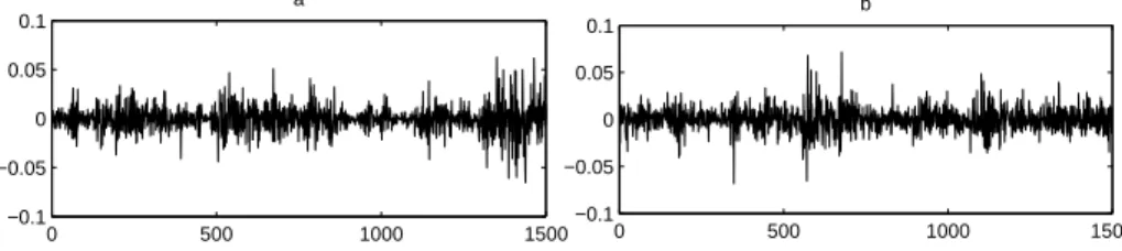
Figure 11: Simulation with Multiplicative Cascade Model and Real Data: Daily Returns 0 500 1000 1500 −0.1 −0.05 0 0.05 0.1 a 0 500 1000 1500 −0.1 −0.05 0 0.05 0.1 b

Left (a): daily returns on index CAC40 (source: Euronext, values of index CAC40 from 20/03/95 to 24/02/05). Right (b): daily returns, simulated with MCM at 14 horizons (from 15 minutes to 256 days). Returns are simulated for every 15 minutes and then are aggregated to daily time intervals.

Figures 11 and 12 show the results of simulation of MCM, compared with real data of index CAC40. The number of horizons in simulation is equal to 14, which allows to fit the speed of decay in the ACF, and other parameters are cal-ibrated so as to match unconditional long-term estimates of the first two sample moments in the returns’ distribution. Note that the figure shows the ACF for returns, aggregated into daily intervals, whereas the simulation itself was carried out at 15-minutes frequencies. This illustrates the most important property of the volatility cascade: clustering of volatility and long-range dependence robust to time aggregation, i.e. coexisting at multiple horizons.

The MCM, described above, is called log-normal, because disturbances to volatility are log-normal. This does not mean that that the resulting distribution of returns is log-normal. Nothing prevents from specifying the model in a way that provides for fat tails at short horizons (see more about it below). In a form described above MCM allows to simulate data, corresponding to the observed financial time series in many properties. But its practical use is complicated

Figure 12: Simulation with Multiplicative Cascade Model and Real Data: Sam-ple ACF 0 20 40 60 80 100 0 0.1 0.2 0.3 0.4 0.5 a 0 20 40 60 80 100 0 0.1 0.2 0.3 0.4 0.5 b

Left (a): sample ACF for the magnitudes of daily returns on index CAC40 (source Euronext, daily values of index CAC40 from 20/03/95 to 24/02/05). Right (b): sample ACF for data, simulated with MCM at 14 horizons (from 15 minutes to 256 days). Returns are simulated for every 15 minutes and then are aggregated to daily time intervals. ACF is computed for daily data.

The link between MCM (here we talk about multiplicative cascade in more general sense, not focused on Breymann et al. (2000) specification, described above) and multifractal processes is studied in Muzy et al. (2000). Consider dyadic horizons of length τn = 2−nτ0. The increment of some process Xt on

interval τk, denoted δkXt, is linked to the increment on the longest scale through

equation: δkXt= Ã k Y i=1 Wi ! δ0Xt (42)

with Wi some iid stochastic factor. In MCM the stochastic volatility process

was defined in a similar way. The expression (42) can be rewritten in terms of a simple random walk in logarithms of local volatility:

ωt,k+1= ωt,k+ ln Wk+1 (43)

with ωt,k = 1₂ln(|δkXt|2). Notice that equation (41) with new notations

cor-responds to Cov (ωt+δt,k, ωt,k). If disturbances ln Wi are normally distributed

N (µ, σ2_{), the distribution density ω}

t,k denoted Pk(ω), satisfies:

Pk(ω) =¡N(µ, σ2)∗k∗ P0¢ (ω) (44)

with ∗ denoting the convolution operator, defined for two function f(t) and g(t) by the expression (f ∗ g)(t) = R f(u)g(t − u)du. Now it is straightforward to show that that equation (44) corresponds to the definition of multifractality in (26) with log-normal propagator of the form:

Gτk,τ0= N (µ, σ

2₎∗k _{= N (kµ, kλ}2_{) (45)}