Polygonization of Remote Sensing Classification Maps by Mesh Approximation

HAL Id: hal-01530460

https://hal.inria.fr/hal-01530460

Submitted on 31 May 2017

HAL is a multi-disciplinary open access

archive for the deposit and dissemination of

sci-entific research documents, whether they are

pub-lished or not. The documents may come from

teaching and research institutions in France or

abroad, or from public or private research centers.

L’archive ouverte pluridisciplinaire HAL, est

destinée au dépôt et à la diffusion de documents

scientifiques de niveau recherche, publiés ou non,

émanant des établissements d’enseignement et de

recherche français ou étrangers, des laboratoires

publics ou privés.

Polygonization of Remote Sensing Classification Maps

by Mesh Approximation

Emmanuel Maggiori, Yuliya Tarabalka, Guillaume Charpiat, Pierre Alliez

To cite this version:

Emmanuel Maggiori, Yuliya Tarabalka, Guillaume Charpiat, Pierre Alliez. Polygonization of Remote

Sensing Classification Maps by Mesh Approximation. ICIP 2017 - IEEE International Conference on

Image Processing, Sep 2017, Beijing, China. pp.5. �hal-01530460�

POLYGONIZATION OF REMOTE SENSING CLASSIFICATION MAPS BY

MESH APPROXIMATION

Emmanuel Maggiori

, Yuliya Tarabalka

, Guillaume Charpiat

, Pierre Alliez

_{Inria Sophia Antipolis-M´editerran´ee, TITANE team}

2

_{Inria Saclay, TAO team}

ABSTRACT

The ultimate goal of land mapping from remote sensing im-age classification is to produce polygonal representations of Earth’s objects, to be included in geographic information sys-tems. This is most commonly performed by running a pix-elwise image classifier and then polygonizing the connected components in the classification map. We here propose a novel polygonization algorithm, which uses a labeled trian-gular mesh to approximate the input classification maps. The mesh is optimized in terms of an `1norm with respect to the

classifiers’s output. We use a rich set of optimization oper-ators, which includes a vertex relocator, and add a topology preservation strategy. The method outperforms current ap-proaches, yielding better accuracy with fewer vertices.

Index Terms— Remote sensing image classification, polygon generalization, geographic information systems

1. INTRODUCTION

One of the central problems in remote sensing is the assign-ment of a thematic class to every pixel in a satellite or aerial image, typically referred to as classification [1]. One of the most important applications is to integrate the data into geo-graphic information systems (GIS), which requires to repre-sent the detected objects as polygons.

Some object detection techniques in remote sensing im-agery directly produce polygonal data, e.g., by fitting rectan-gles to the image [2]. However, to account for more general shapes one must first classify every pixel and then polygonize the classification map. Moreover, with the advent of deep learning, the pixelwise classification of remote sensing im-agery is becoming more and more effective [3, 4]. The usual approach is to vectorize a raster object in a naive way, i.e, by creating a polygon with points at every pixel all around the object boundary, and then to simplify such a polygon. This second step is often referred to as polygon generalization [5]. The most common generalization algorithms can be clas-sified into local and global processing routines. Local rou-tines, such as the radial distance [6] and Reumann-Witkam [7]

The authors would like to thank CNES for funding the study. Pl´eiades images are CNES (2012 and 2013), distribution Airbus DS / SpotImage

methods, compare subsequent points in a polygon to decide if one of them may be eliminated. Visvalingam-Whyatt [8] and Douglas-Peucker [9] are global greedy routines that mea-sure the effect of including each point on the entire polygon and not only with respect to the nearest neighbors. These techniques are implemented in most GIS packages (e.g., GRASS, QGIS and ArcGIS), Douglas-Peucker being the most commonly used method by the community [6]. It has been adapted to preserve topology and to generate non-self-intersecting polygons [10, 11].

We here propose a polygonization technique based on the approximation of a triangular mesh to the classification maps. While previous methods simplify based on some measure of distance between the complex and approximated polygon boundaries, our method proceeds in an integral manner, i.e., considering the approximation error over the entire surface of the image. In addition, instead of just removing vertices, our approach consists of a rich set of operators which also allows their relocation, permitting to compensate for the imprecisions in the classification map.

2. POLYGONIZATION AS MESH APPOXIMATION Let us consider a triangular mesh T , consisting of a set of triangles {ti}, overlaid on top of an image to partition it (see

e.g. Fig. 4). There is a set of class labels L and we define C(l, x, y) to be the cost associated to assigning a certain label l ∈ L to a pixel (x, y) in the image. We also assign a single label lt to every triangle t. The cost of such an assignment

is simply the cost of assigning the label uniformly to all the points inside the triangle. We naturally assume that the label assigned to each triangle is the one with the lowest cost. Our goal is to find the triangulation that minimizes:

E(T ) =X t∈T  min lt∈L Z Z x,y∈t C(lt, x, y)dxdy + λ  . (1)

For each triangle we sum the cost incurred by assigning the optimal label to it, plus an extra weight λ per triangle. Adding λ implies that the mere existence of a triangle has a cost, in-dependently of its label, and is thus used as a regularization term to set the desired coarseness of the mesh.

t1 t2 t3 t4 t5

T l_1,3,5=0

l2,4=1

∫

∫

∫

Fig. 1: Illustration of the `1cost on a 1-D triangulation.

(a) (b)

Fig. 2: Operators: edge flip (a) and half-edge collapse (b).

We here consider that a classifier has been used to es-timate P (l, x, y), the probability P (l, x, y) of assigning a certain label l ∈ L to a point (x, y) in the image (s.t. P

l∈LP (l, x, y) = 1 and P (l, x, y) ≥ 0, ∀x, y, l). We here

define the cost as follows:

C(l, x, y) = ||1 − P (l, x, y)||1, (2)

which can be seen as the volume contained between the clas-sifier’s probability surface and the piecewise constant approx-imation implied by the labeled mesh. Fig. 1 illustrates an ex-ample of such cost in 1-D. Let us remark that in addition to using the fuzzy probabilities of a classifier, we can also use a hard classification map (i.e., a unique class assigned to each pixel) by supposing that the probability was set to 1 for the assigned class and 0 for the rest.

The triangular mesh is iteratively optimized by perform-ing a local search, startperform-ing from an initial fine lattice. We sim-ulate a number of changes that transform the mesh, from T to T0, and construct a modifiable priority queue on the energy variation ∆E = E(T0) − E(T ) associated to each change. We can restrict the calculation of ∆E to the triangles affected by the change, given the sum over independent triangles in (1). The highest priority change is first extracted from the queue and applied to the mesh. Note that we must relabel the affected triangles and update those elements in the queue that may have been altered as a side effect. This is iterated until there are no changes left. We only consider changes that im-mediately improve T (i.e., ∆E < 0) and that produce a valid triangulation (e.g., they do not lead to overlapping triangles). The first two types of changes we consider are the edge flipand half-edge collapse [12, 13] operators (see Fig. 2). We can transform a triangulation to become any possible simpli-fied triangulation just by flips and collapses, as soon as the vertices are on fixed locations [12], making those two types of operators particularly appealing. However, we also add a vertex relocationoperator that computes a new position for a certain vertex. This increases the expressiveness of the fam-ily of operators, compensating the limitation of flips/collapses that simply recombine predetermined vertices. For example, vertex relocation allows us to start the optimization from a relatively coarse mesh and yet achieve similar (or even better)

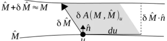
δ ^M⋅^n δ ^M du u ^ M ^ M +δ ^M ≈M ^ n δA(M , ^M )_u

Fig. 3: Elementary area variation δA generated by δ ˆM .

results than if we departed from a fine mesh (e.g., a vertex on every pixel) and only used flips and collapses. Note that dif-ferent types of operators can be mixed together in the queue, or they can be applied at will in subsequent stages of the al-gorithm.

Once the mesh has been optimized, the connected com-ponents of triangles with the same class label are outputted as polygonal objects of such class.

3. VERTEX RELOCATION

While the application of flip and collapse moves is self-explanatory, we dedicate this section to our vertex relocation algorithm.

We first see the object boundaries in the classification map as curves in the plane, an object being a connected component of pixels of the same class. We also see the boundaries of objects in the triangulation as curves in the plane. Denoting by M the “real” boundaries on the classification map and by

ˆ

M the ones implied by the labeled triangulation, our goal is to modify ˆM so that it approaches M . We also use the `1-norm

and seek to minimize the area A(M, ˆM ) contained between the two curves. We adapt the algorithm from [14], where a volume criterion was used to simplify 3-D meshes.

Given a curve ˆM parametrized by u, we define δ ˆM (u) as the displacement of a point that belongs to such curve (see Fig. 3), with the goal of approximating M . We assume that

ˆ

M can be locally approximated by its tangent, and define du to be a small displacement along the tangent. The variation of area δA(M, ˆM )uincurred by performing the displacement

δ ˆM (u) corresponds to the parallelogram generated by δ ˆM (u) and du. The area of such parallelogram is |δ ˆM (u) · ˆn| · du, being ˆn(u) a vector normal to ˆM . Since the variation of area δA(M, ˆM )u may be positive or negative (because δ ˆM (u)

may approach or move ˆM away from M ), we define: δA(M, ˆM )u= η(u)(δ ˆM (u) · ˆn)du, (3)

where η returns -1 if if ˆn points toward the area embedded between M and ˆM and +1 otherwise, since it would be re-ducing and increasing the area, respectively (assuming ˆn is oriented so that δ ˆM · ˆn is positive). The total area variation upon applying all displacements is:

δA(M, ˆM ) = Z

u

η(u)(δ ˆM (u) · ˆn)du. (4) However, while (4) applies to any curve, in our piecewise lin-ear case when we move a vertex Xithe points along adjacent

edges move accordingly. In fact, the δ ˆM (u) of a point inside a segment XaXbis a linear combination of δXaand δXb:

δ ˆM (u) = λa(u)δXa+ λb(u)δXb, (5)

where λa,b(u) are shape functions [15] such that λi is 1 on

Xiand linearly decreases to zero until reaching the following

and previous vertices in the curve. This interpolates Xa and

Xbbased on their relative distance to δ ˆM (u).

If we differentiate (4) with respect to a particular vertex Xiand use (5), we get:

∂A(M, ˆM ) ∂Xi

= Z

u∗

η(u)λi(u)ˆn(u)du. (6)

We restrict the domain of integration to the points in edges adjacent to Xi (which we denote by u∗) because only there

λi(u) is nonzero.

Note that the challenge of evaluating (6) reduces to the computation of η(u). We evaluate (6) as follows: first we take a discrete number of points along every edge adjacent to Xi. From each of these points we “shoot a ray” to decide to

which side lies the curve we want to approach. For example, in the 2-class case we just shoot rays in opposite directions and see which one hits first the 0.5 probability level, where there is a change of classes and hence an object boundary.

The iterative optimization of Xiis performed by gradient

descent. Being k the iteration number, we set:

X_i(k+1)= X_i(k)− α(k)∂A

(k)_{(M, ˆM )}

∂Xi

, (7)

where α(k) _{is an adaptive step that starts at α}(0) _{= α and}

is multiplied by a factor γ < 1 whenever an oscillation is detected (∂A_∂X(k)

i ·

∂A(0) ∂Xi < 0).

As with the other operators, these moves are simulated and added to the priority queue based on the associated ∆E.

4. TOPOLOGY PRESERVATION

While some mesh approximations may be energetically op-timal in terms of (1), they may be unpleasant from a quali-tative point of view because they modify the topology of the objects. A notorious case is that nearby buildings are often merged together into one single object, or buildings that were not adjacent in the initial mesh are connected in the simplified mesh.

We deal with this situation by preventing changes that incur in topological changes. To describe the topology of the objects of a certain class we use the Euler characteristic χ = V − E + F , where V , E and F are the number of vertices, edges and faces in a mesh, respectively [16]. For example, when there is a single object of a class, χ = 1, for two separate objects χ = 2, for one object with two holes χ = −1. For each class we must verify that χ does not change

(a) Color input (b) Initial mesh (c) Edge flips

(d) Vertex relocations (e) Edge collapses

Fig. 4: Effect of applying the different mesh operators.

as a result of applying an operator. We do this in practice by counting the changes ∆V , ∆E and ∆F incurred by the op-erator, only doing this locally on the elements that may have changed as a result of its application. We then verify that ∆χ = ∆V − ∆E + ∆F = 0. We count those vertices, edges and faces that are adjacent to a triangle labeled with the class for which we are verifying the topological change.

Notice that we may adjust the tolerance to topological changes by the coarseness of the initial mesh. For example, if a small hole in the classification map is ignored in the initial labeling, it will remain like that. In other words, one reason-ably expects that the initial mesh is finer than what is consid-ered to be the minimum object size.

5. EXPERIMENTS

We experiment on a dataset of Pl´eiades satellite imagery, manually labeled into two classes: building/not building. We use the classification maps obtained by the two-scale convolutional neural network (CNN) presented in [4].

Let us first illustrate the effect of applying the different operators. Fig. 4(a) shows a piece of color image from the dataset in [4]. In Fig. 4(b) we show the corresponding classi-fication map outputted by the CNN, overlayed with the initial mesh (a lattice with one vertex every 10 pixels). Through the samples we amplify the fragment indicated by the green square on Fig. 4(a). Upon filling the priority queue with flips and applying them till the queue is empty, we get the mesh on Fig. 4(c). On this mesh we perform vertex relocations in a similar fashion, obtaining the mesh in Fig. 4(d). Finally, collapses are done as shown in Fig. 4(e).

We now compare our polygonization method with com-peting methods. Our algorithm is as follows: we first per-forms a stage involving only edge flips, followed by a stage of vertex relocations (as in Fig. 4). Then we perform edge collapses and, after each collapse we immediately simulate a

0 1000 2000 3000 4000 5000 6000 99.4 99.42 99.44 99.46 99.48 99.5 99.52 99.54 99.56 99.58 Number of vertices Accuracy (%) Mesh approximation Douglas−Peucker Visvalingam−Whyatt Radial distance Reumann−Witkam

Fig. 5: Performance comparison.

(a) Color input (b) Classif. map (c) DP, thr. 3 (d) DP, thr. 7 (e) Mesh approx.

Fig. 6: Visual comparison (“DP, thr. 3”: Douglas Peucker with threshold 3).

vertex relocation on the collapsed node (because we assume that the collapsed node does not end up in the optimal location right away). We can alternatively just mix all the operations together, but we found this way to be more efficient and ele-gant because the first two stages better align the initial mesh to the classification map at very low cost, prior to start to col-lapse edges. We start from a fine mesh (one vertex per pixel, in a band around object boundaries).

For vertex relocation we shoot five rays per segment (weighting them based on their distance du) and perform gradient descent with α = 0.1, γ = 0.1, stopping when α(n)_{< 0.0001 or the displacement is below 0.01 pixels.}

We compare our polygonization method with the stan-dard techniques used in geographic information systems (GIS). We first vectorize the rasters with GDAL library’s function gdal polygonize and then use GRASS and QGIS implementations of the simplification methods mentioned in the introduction.

In Fig. 5 we plot the accuracy of the polygonal approxi-mation as a function of the amount of vertices (e.g., for dif-ferent values of λ in Eq. 1). This is done on the entire test set of [4]. Since we have ground truth data, accuracy is directly measured as the percentage of correctly classified pixels when rasterizing the polygons. Our algorithm outperforms the other techniques, including the popular Douglas-Peucker and Vasvalingam-Whyatt which are the most accurate among them. The advantage is significant, for example, for a de-sired accuracy of 99.54%, Douglas-Peucker requires 1200 vertices while our technique achieves the same accuracy with only 700. This is also appreciated visually. Figs. 6(a-b) show a piece of color image and the corresponding classifi-cation map. Figs. 6(c) and (d) show the result of applying Douglas-Peucker with two different threshold parameters, and Figs. 6(d) illustrates our results. The parameters of Douglas-Peucker were selected so as to provide a similar accuracy to our method (in Fig. 6c) and a similar amount of vertices than our method (in Fig. 6d). We observe that for a similar accuracy there are too many vertices compared to Fig. 6(d), while for the same number of vertices the polygons by Douglas-Peucker do not represent the underlying objects well, explaining the gap between the curves in Fig 5.

Fig. 7: Examples of color inputs (left) and approximation without (center) and with (right) topological constraints.

0 50 100 150 200 250 99.35 99.4 99.45 99.5 99.55 99.6 Coarseness (λ) Accuracy (%) Mesh approximation Mesh approximation (no vertex reloc.)

Fig. 8: Approximation with and without vertex relocation.

In Fig. 7 we illustrate the effect of removing the topologi-cal constraints described in Sec. 4, where we observe that our methodology effectively outputs polygons that better convey the topology of the underlying objects. Finally, as depicted in Fig. 8, the use of vertex relocation consistently outperforms an equivalent algorithm where vertex relocation is removed.

6. CONCLUDING REMARKS

We presented a mesh approximation algorithm to polygonize remote sensing classification maps. The polygonal objects are more accurate than the current methods used in the GIS community, and provide good approximations of the objects with a significantly lower number of vertices. This is partly because we allow vertices to be located anywhere and not just exactly on the boundary of the original raster objects. Another essential difference of our technique and is that we measure the approximation error in an integral manner over the entire surface of the image.

In the future we plan to reinforce regularity relationships (e.g., parallelism, right angles) in the framework, learned from training data, as well as to introduce machine learning in the decision of applying the different operators.

7. REFERENCES

[1] Dengsheng Lu and Qihao Weng, “A survey of im-age classification methods and techniques for improv-ing classification performance,” International journal of Remote sensing, vol. 28, no. 5, pp. 823–870, 2007. [2] Mohammad Awrangjeb, Mehdi Ravanbakhsh, and

Clive S Fraser, “Automatic detection of residential buildings using lidar data and multispectral imagery,” ISPRS Journal of Photogrammetry and Remote Sensing, vol. 65, no. 5, pp. 457–467, 2010.

[3] Michele Volpi and Devis Tuia, “Dense semantic la-beling of subdecimeter resolution images with convo-lutional neural networks,” IEEE Transactions on Geo-science and Remote Sensing, vol. 55, no. 2, pp. 881– 893, 2017.

[4] Emmanuel Maggiori, Yuliya Tarabalka, Guillaume Charpiat, and Pierre Alliez, “Convolutional neural net-works for large-scale remote-sensing image classifica-tion,” IEEE Transactions on Geoscience and Remote Sensing, vol. 55, no. 2, pp. 645–657, 2017.

[5] Martin Galanda, Automated polygon generalization in a multi agent system, Ph.D. thesis, Zurich: Zurich Uni-versity, 2003.

[6] Wenzhong Shi and ChuiKwan Cheung, “Performance evaluation of line simplification algorithms for vector generalization,” The Cartographic Journal, vol. 43, no. 1, pp. 27–44, 2006.

[7] K Reumann and APM Witkam, “Optimizing curve seg-mentation in computer graphics,” in Proceedings of the International Computing Symposium, 1974, pp. 467– 472.

[8] M Visvalingam and JD Whyatt, “Line generalisation by repeated elimination of the smallest area,” The Carto-graphic Journal, vol. 30, no. 1, pp. 46–51, 1992. [9] David H Douglas and Thomas K Peucker, “Algorithms

for the reduction of the number of points required to rep-resent a digitized line or its caricature,” Cartographica: The International Journal for Geographic Information and Geovisualization, vol. 10, no. 2, pp. 112–122, 1973. [10] Alan Saalfeld, “Topologically consistent line simplifica-tion with the douglas-peucker algorithm,” Cartography and Geographic Information Science, vol. 26, no. 1, pp. 7–18, 1999.

[11] Shin-Ting Wu and Mercedes Roc´ıo Gonz´alez M´arquez, “A non-self-intersection douglas-peucker algorithm,” in SIBGRAPI. IEEE, 2003, pp. 60–66.

[12] Mario Botsch, Leif Kobbelt, Mark Pauly, Pierre Alliez, and Bruno L´evy, Polygon mesh processing, CRC press, 2010.

[13] Antonio Wilson Vieira, Luiz Velho, H´elio Lopes, Geo-van Tavares, and Thomas Lewiner, “Fast stellar mesh simplification,” in SIBGRAPI. IEEE, 2003, pp. 27–34. [14] Pierre Alliez, Nathalie Laurent, Henri Sanson, and

Fran-cis Schmitt, “Mesh approximation using a volume-based metric,” in Proceedings of Seventh Pacific Con-ference on Computer Graphics and Applications.IEEE, 1999, pp. 292–301.

[15] Thomas JR Hughes, The finite element method: linear static and dynamic finite element analysis, Dover Pub-lications, 2012.

[16] David S Richeson, Euler’s gem: the polyhedron formula and the birth of topology, Princeton University Press, 2012.