Land use dynamics and the environment

HAL Id: hal-01074190

https://hal.archives-ouvertes.fr/hal-01074190

HAL is a multi-disciplinary open access archive for the deposit and dissemination of sci-entific research documents, whether they are pub-lished or not. The documents may come from teaching and research institutions in France or abroad, or from public or private research centers.

L’archive ouverte pluridisciplinaire HAL, est destinée au dépôt et à la diffusion de documents scientifiques de niveau recherche, publiés ou non, émanant des établissements d’enseignement et de recherche français ou étrangers, des laboratoires publics ou privés.

Land use dynamics and the environment

Carmen Camacho, Agustín Pérez-Barahona

To cite this version:

Carmen Camacho, Agustín Pérez-Barahona. Land use dynamics and the environment. 2014. �hal-01074190�

LAND USE DYNAMICS AND THE ENVIRONMENT

Carmen CAMACHO

Agustín PÉREZ-BARAHONA

September 2014

Cahier n°

2014-25

ECOLE POLYTECHNIQUE

CENTRE NATIONAL DE LA RECHERCHE SCIENTIFIQUE

DEPARTEMENT D'ECONOMIE

Land use dynamics and the environment

Carmen Camacho

CNRS, Universit´e Paris 1 Panth´eon-Sorbonne (France)

Agust´ın P´erez-Barahona

INRA-UMR ´Economie Publique and ´Ecole Polytechnique (France)⇤

September 26, 2014

Abstract

This paper builds a benchmark framework to study optimal land use, encom-passing land use activities and environmental degradation. We focus on the spatial externalities of land use as drivers of spatial patterns: land is immobile by na-ture, but local actions a↵ect the whole space since pollution flows across locations resulting in both local and global damages. We prove that the decision maker problem has a solution, and characterize the corresponding social optimum tra-jectories by means of the Pontryagin conditions. We also show that the existence and uniqueness of time-invariant solutions are not in general guaranteed. Finally, a global dynamic algorithm is proposed in order to illustrate the spatial-dynamic richness of the model. We find that our simple set-up already reproduces a great variety of spatial patterns related to the interaction between land use activities and the environment. In particular, abatement technology turns out to play a central role as pollution stabilizer, allowing the economy to reach a time-invariant equilibrium that can be spatially heterogeneous.

Keywords: Land use, Spatial dynamics, Pollution. Journal of Economic Literature: Q5, C6, R1, R14.

⇤_{Corresponding author at: INRA-UMR210 ´Economie Publique, Avenue Lucien Br´etigni`eres, 78850 Thiverval Grignon, France; e-mail:}

1

Introduction

Land use activities are usually defined as the transformation of natural landscapes for human use or the change of management practices on human-dominated lands (Foley et al., 2005). It is widely accepted that these activities have greatly transformed the planet’s surface, encompassing the existence and evolution of spatial patterns (for in-stance, Plantinga, 1996; Kalnay and Cai, 2003; and Chakir and Le Gallo, 2013). In this regard, Spatial Economics analyses the allocation of resources over space as well as the location of economic activity and, thus, the formation of spatial patterns. In par-ticular, great e↵ort has been devoted to understanding firms’ location, transport costs, trade, and regional and urban development (Duranton, 2007). However, the mechanisms behind the interaction between land use and the environment that can induce spatial patterns, designated in our paper as spatial drivers, are still far for being understood. In this paper we contribute to the theoretical foundations of land use change and the environment by considering the interaction between land use activities and pollution. To this end we will develop a theoretical model that focuses on the spatial externalities of land use as drivers of spatial patterns.

There is an abundant literature on the interaction between land use and pollution. Agricultural research in particular has devoted great attention to the e↵ects of pol-lution on agricultural land use (for instance, Adams et al., 1986; and Deschˆenes and Greenstone, 2007). About the environmental influence of land use, many papers have identified significant environmental impacts of land use (among others, Matson et al., 1997; and Kalnay and Cail, 2003). Moreover, Foley et al. (2005) point out that the e↵ects of environmental degradation due to land use are global but also regional/local. Although this literature has been very fruitful, the dominant approach has been empir-ical. There is indeed a general agreement about the lack of explicit modelling of the spatial drivers behind the interaction between land use and pollution. Closely related to the integrated assessment approach, bottom-up models of agricultural economics (for instance, de Cara et al., 2005) have contributed to the understanding of the spatial drivers of land use. However, these models focus on partial equilibrium (mainly the supply side) and do not completely consider the intertemporal dimension of the prob-lem. In this paper we use an alternative approach based on the Dynamic Spatial Theory (see Desmet and Rossi-Hansberg, 2010, for a survey).

Within this theory, considering the forward-looking dimension of agents’ decisions, the natural spatial generalization of the Ramsey model is presented in Brito (2004) and

Boucekkine et al. (2009 and 2013a). Both include a policy maker who decides the trajectory for consumption at each location. The main feature of these models is the spatial dynamics of capital, which flows in space to meet optimal decisions according to a partial di↵erential equation (PDE). Although these sophisticated models are very promising, several technical problems have been identified (Boucekkine et al., 2013b). In particular, the application of parabolic PDEs in this new field has opened a set of questions still not solved by the mathematical literature. To date, there have been few pragmatic approaches that provide alternative set-ups. For instance, Costello and Polasky (2008) provide a dynamic framework to study the optimal harvesting of re-newable resources in a stochastic spatial (partial equilibrium) model. Taking advantage of the special structure of the problem, they are able to analytically characterize the equilibrium. Desmet and Rossi-Hansberg (2009, 2010 and 2013), more in line with the spatial Ramsey model, follow the idea of imposing enough structure to the spatial prob-lem (through factors’ mobility, di↵usion of technology, and land and firm ownership) as well. Agents are assumed to be myopic. While each location solves a static problem, their model is dynamic in time. Indeed, each location decides the optimal amount to consume, how much to invest in R&D, and how much to save, taking land revenues, prices and salaries as given. Finally, all savings are coordinated by a cooperative that invests along the space. Even if this approach allows us to understand some important geographic features, the structure of their framework makes the planner’s problem in-tractable (see also Desmet and Rossi-Hansberg, 2012). Another interesting alternative is the one followed by Brock and Xepapadeas (2008 and 2010). Considering Derzko et al. (1984), they approximate (linear quadratic) the original nonlinear optimal control problem, around a time-invariant equilibrium. However, as we will show later, neither existence nor uniqueness of time-invariant solutions are ensured in an environmental spatial Ramsey framework.

We use in this paper the spatial generalization of the Ramsey model in order to understand the spatial drivers behind land use and the environment. To the best of our knowledge, our paper provides a first analytically tractable general equilibrium framework of land use that, without approximating the original optimal control problem, encompasses (i) spatial and time dimensions which are presented in a continuous manner, (ii) spatial externalities due to pollution and abatement activities, and (iii) the social optimum. Our starting point is the Spatial Ramsey model in Boucekkine et al. (2009 and 2013a). We propose a benchmark framework in continuous time and space to study optimal land use. Each location is endowed with a fixed amount of land, which is

allocated among production, pollution abatement, and housing. Although the unique production input (land) is spatially immobile by nature, this is a model of spatial growth where local actions a↵ect the entire space through pollution. Indeed, we assume that the production generates local pollution, which flows across locations. In this regard, we illustrate the di↵usion mechanism by means of the well-known Gaussian Plume equation (see Sutton, 1947a,b). Finally, we consider that local pollution damages production due to its negative e↵ect on land productivity. Moreover, we assume that pollution as a whole (global pollution) may also reduce production. This indirect consequence of pollution can be linked, for instance, to the negative e↵ect of anthropogenic GHGs on climate change.1

We prove the existence of a social optimum when the planning horizon is finite. The policy maker decisions are characterized by the Pontryagin conditions. We additionally extend our analytical results to the time-invariant equilibrium. As observed above, this particular equilibrium is crucial to apply solution methods based on approximations of the original problem around a time-invariant equilibrium. We show in this respect that the existence and uniqueness of time-invariant solution are not guaranteed in general. Finally, to illustrate the richness of our model, we undertake numerical simulations. To this end we adapt the methodology first developed in Camacho et al. (2008) to the current problem. Our algorithm is an alternative framework to other numerical tools that focus on the local dynamics around a time-invariant solution. This numerical analysis is actually global, where we simulate the entire trajectory of the states, controls, and co-states from their initial distributions until they eventually reach, or not, a time-invariant equilibrium. With the numerical tool in hand, we study the di↵erent drivers of spatial heterogeneity. We find, among other things, that the abatement technology stands out as a fundamental element to achieve time-invariant solutions, which are compatible with the emergence of long-run spatial patterns. Moreover, even if our paper focuses on land use dynamics, many simulated scenarios are consistent with the predictions of spatial models of natural resources such as the harvesting stochastic spatial approach of Costello and Polasky (2008).

The paper is organized as follows. Section 2 describes the economic model. Section 3 is devoted to the analytical results of our paper. In Section 4 we introduce the algorithm that is applied in the numerical exercises of Section 5. Finally, Section 6 concludes.

1_{According to Akimoto (2003), tropospheric ozone, methane and CO are well-known examples of}

pollutants that flow across locations. Methane and CO have both local and global e↵ects. Moreover, CO a↵ects the oxidizing capacity of the atmosphere, raising the lifetime of GHGs.

2

The model

We assume that there exists a continuum of locations along a unidimensional region R_{✓ R. We also consider that R is an open and connected real set.}2 _{Each location has a}

unit of land, which can be devoted to three di↵erent activities: production, housing and pollution abatement.3 _{For simplicity, we shall assume that the space required for housing}

at each location is equal to its population density f (x). We also consider no population growth in this paper. There exists a unique consumption good the production of which only requires land and that we denote by F (l). The remainder of the land is used to

abate pollution G(1 l f (x)).

Pollution has two dimensions in our model. The local dimension (local pollution) comes directly from the production of the consumption good. For the sake of simplicity, we assume that each unit of production generates one unit of pollution. It damages production due to the negative e↵ect on land productivity. Moreover, even if land is spatially immobile, local decisions a↵ect the whole space since the pollutant travels across space. We describe the spatial dynamics of pollution by means of a well-known model in physics called the Gaussian plume. It is a standard mathematical description of the dispersion of airborne contaminants (for instance, Arya, 1999; and Stockie, 2011). But it is also used to model the spread of pollutants in aquifers and porous soils and rocks, as well as for nuclear contaminants. According to this model, the dynamics of the pollution at location x in time t, p(x, t), is given by the following second-order partial di↵erential equation (PDE) of parabolic type:

pt(x, t) pxx(x, t) = E(x, t), (1)

where pt and pxx denote, respectively, @p(x, t)/@t and @2p(x, t)/@x2, and E(x, t) are

the emissions in time t 0 of a single source located at x. The interpretation of

equation (1) is the following (see Smith et al., 2009, for a detailed description from an environmental economic perspective). The Gaussian plume model comprises two common dispersal mechanisms of pollutants: di↵usion and /or advection. Di↵usion is the spread of a pollutant through regions where its concentration is high to regions

2_{Results can be easily extended to the case R ✓ R}n_{, n > 1, and to the case in which R is not}

connected but the union of connected subsets in R.

3_{In this simplified set-up, the land devoted to abatement may be interpreted as being pollution}

removal due to the presence of, for instance, prairies and forests (see Nowak et al., 2006; and Ragot and Schubert, 2008). In general, one can also consider that abatement activities require physical space (land in our model).

of lower concentration (Fick’s law), while advection is the flux of contaminants due to wind, ocean currents, etc. As in Brock and Xepapadeas (2008 and 2010), and Smith et al. (2009), we focus on di↵usion. The term pxx(x, t) in (1) reflects indeed the

spread due to concentration di↵erential. We pay attention to this dispersal mechanism because our approach is about growth and the long-term response of the economy: the elements behind advection (e.g., wind velocity and direction) are extremely variable, in particular in the short-run, and the time horizon usually considered in this type of problems minimizes this e↵ect. For advection, the other polar case, see for instance Costello and Polasky (2008) in the context of the spatial economics of natural resources (fish).4

Additionally, pollution may also harm production as a global pollutant (e.g., anthro-pogenic GHGs). We then allow for the distinction between local and global pollution, where global pollution is naturally defined as:5

P (t) = Z

R

p(x, t)dx. (2)

We introduce pollution damages in production using a damage function ⌦(p, P, x), where 1 ⌦ represents the share of foregone production due to local and global pollution.6

If we denote by A(x, t) the total factor productivity at location x at time t, we have that this location produces ⌦(p, P, x)A(x, t)F (l) units of final good when it devotes an amount l of land to production. For simplicity reasons we shall assume that the abatement technology is not a↵ected by pollution. In the remaining of the paper we make the following standard assumptions regarding the production functions:

(H1) Functions F and G are positive, increasing, concave, and their first and second derivatives exist and are non negative, that is:

F (_{·) 2 C}2, F (0) = 0, F0(_{·) > 0, F}00(_{·)  0, lim} s_!0F 0_{(s) =1, lim} s_!1F 0_{(s) = 0,} G(·) 2 C2_{, G(0) = 0, G}0_{(·) > 0, G}00_{(·)  0, lim} s_!0G 0_{(s) =1, lim} s_!1G 0_{(s) = 0.}

4_{The Gaussian plume model can be also used in natural resource management. Smith et al. (2009)}

observe that advection can be eventually modeled “through di↵erences in rates of dispersal”, i.e., D(x, t)pxx(x, t), where D(x, t) is the di↵usion coefficient. However, this would require further physical

assumptions that are beyond the scope of our paper.

5_{Well-known pollutants with mostly global e↵ects are CO}

2and CFCs (see, among others, Nordhaus,

1977; and Akimoto, 2003). However, air contaminants in general (including tropospheric ozone and NOx) are examples of local pollutants that flow among locations.

6_{Notice that the productivity loss may also encompass the negative e↵ect of pollution on individuals’}

health (among others, Pope, 2000; and Evans and Smith, 2005). However, we do not explicitly consider this e↵ect in our paper.

(H2) ⌦(p, P, x) is twice di↵erentiable with respect to p and P ; and decreasing in each factor: ⌦1(p, P, x) = @⌦(p,P,x)_@p < 0, ⌦2(p, P, x) = @⌦(p,P,x)_@P < 0. Function ⌦(p, P, x)

is defined on R+_{⇥ R}+_{⇥ R and takes values in [0, 1].}

Assumption (H1) is the usual hypothesis of positive and non-increasing marginal prod-ucts, together with the Inada conditions. (H2) assumes that both local and global pollution a↵ect negatively production. Moreover, it is also considered that this damage is a smooth function.

Boucekkine et al. (2009 and 2013a) assume that each location produces its own consumption in the social optimum. Social welfare, however, may still increase under the possibility of spatial reallocation of production. We therefore enlarge the set of feasible abatement and production decisions by allowing for consumption “imports”. Indeed, we assume that the policy maker collects all production and re-allocates it across locations at no cost:

Z R c(x, t)f (x)dx = Z R ⌦(p, P, x)A(x, t)F (l)dx, (3)

where c(x, t) denotes consumption per capita at location x and time t.7

The policy maker chooses consumption per capita and the use of land at each lo-cation, which maximize the discounted welfare of the entire population. Following Boucekkine et al. (2009), we introduce two discount functions. The spatial discount represents the weight that the policy maker gives to each location. Alongside their paper, we identify this function as the population density f (x) in order to avoid any subjective spatial preferences. Moreover, as in the standard Ramsey model, we consider the usual temporal discount e ⇢t_{, with ⇢ > 0. The policy maker maximizes the lifetime}

discounted utility max {c,l} Z T 0 Z R u(c(x, t))f (x)e ⇢tdxdt + Z R (p, P )(x, T )e ⇢Tdx (4) subject to

7_{In this paper we do not consider transportation costs. However, it is possible to introduce them if}

proportional to the shipped amount of final good, or under other further assumptions. These could be for instance the compulsory gathering of output in a specific location.

P 8 > > > > > > > > > > > < > > > > > > > > > > > : pt(x, t) pxx(x, t) = ⌦(p, P, x)A(x, t)F (l(x, t)) G(1 l f (x)), R Rc(x, t)f (x)dx = R R⌦(p, P, x)A(x, t)F (l)dx, P (t) =R_Rp(x, t)dx, p(x, 0) = p0(x) 0, limx! Rpx(x, t) = 0, (5)

where (x, t)2 R ⇥ [0, T ] and denotes R’s boundaries. In particular, if R = R then

R = { 1, 1}. Moreover, R = {a, b} if R is an open interval (a, b). Following the

standard approach, we consider an instantaneous utility function u : R+ _{! R that is}

increasing and concave. As in Camacho et al. (2008), the function is measurable and everywhere finite. It accounts for the planner’s concern about the state of pollution at the end of the planning period. In the standard Ramsey model, if the policy maker does not state any function , then the optimal solution is such that savings are zero at T and it is the end of the economy (for instance, Acemoglu, 2009). Similarly, if we show no concern about the pollution at the end of the planning period, then pollution will be infinite at T and its shadow price will be zero. Finally, as in Boucekkine et al. (2009), the last expression in (5) is the usual boundary condition: there is no pollution flow in the boundaries of the space.8

3

The social optimum

In this section we present the theoretical contribution of the paper. We first show that there exist a solution to our problem. Moreover, the optimal trajectories are charac-terized by the Pontryagin conditions, involving a system of PDEs. Section 3.2 finally focuses on the time-invariant solution, which is defined as the situation when all vari-ables remain constant in time.9 _{We prove that both existence and uniqueness of this}

solution (that can be spatially heterogenous) are not in general guaranteed. In this

8_{No pollution flow means that lim}

x! Rpx(x, t) is equal to a constant (this is called the Neumann

problem). Without loss of generality, we can assume this constant equal to zero. Notice that, as in Boucekkine et al. (2013a), if space was a circle no boundary condition would be required since the space does not actually have boundaries.

9_{Since we consider a finite planning period, we prefer to use the term “time-invariant”. The}

regard, we provide a sufficient condition that will be used in the numerical part of the paper.

3.1

Optimal trajectories

Let us start by showing, in Proposition 1, that there exist at least a solution to the

social optimum problem. In this regard, we prove that P has a unique solution for

every choice of the couple (c, l). Notice that this outcome is not a direct application of existing results (Camacho et al., 2008) because of some special features of _{P. In} particular our model includes a global variable P , defined as the spatial integral of p. Moreover, in contrast to the previous literature, we consider that the policy maker gathers all production to distribute it later, adding the aforementioned supplementary integral constraint on consumption. Consequently, we first have to transform these two integral constraints into partial di↵erential equations in the proof of the proposition. Afterwards, by imposing the following Assumption (H3), we can apply Theorem 12.1 in Chapter 8 in Pao (1992) to close the proof:

(H3) For all (x, t)_{2 R ⇥ (0, T ], there exist some real constants p}1 > 0, ! > 0, !1 > 0,

!2> 0 and b < 1/4T , such that, as x! R, 0 < p(x, t) p1eb|x 2_| , 0 < ⌦(x, t) !eb|x2|, 0 <|⌦1(x, t)|  !1eb|x 2_| , 0 <|⌦2(x, t)|  !2eb|x 2_| . As in Camacho et al. (2008), and Boucekkine et al. (2009), this is a technical assumption that allows us to avoid explosive solutions in the frontiers of the space. Moreover, we should also observe that the exponential terms in (H3) make this hypothesis not very restrictive. For ease of exposition, we report all proofs details of the paper in the Appendices.

Proposition 1. Under assumptions (H1)-(H3), the problem (4)-(5) has a solution in (x, t)2 R ⇥ (0, T ], for every T < 1.

Once we know that there exists at least a solution to the social optimum, let us characterize the optimal trajectories. In this regard, we use the Ekeland method of variations in Raymond and Zidani (1998 and 2000) to obtain the Pontryagin conditions of problem (4)-(5).10 _{Following this procedure, we write the associated value function}

10_{The Ekeland variational principle (Ekeland, 1974) ensures the existence of a maximum value for V}

V as a function of c, l, p and P as follows: V (c, l, p, P ) =R₀TR_Ru (c(x, t)) f (x)e t_{dxdt +}R R (p, P )(x, T )e Tdx RT 0 R Rq(x, t) [pt(x, t) pxx(x, t) ⌦(p, P, x)A(x, t)F (l(x, t)) + G(1 l f (x))] dxdt RT 0 m(t) ⇥ P (t) R_Rp(x, t)dx⇤dt RT 0 n(t) ⇥R Rc(x, t)f (x)dx R R⌦(p, P, x)A(x, t)F (l(x, t))dx ⇤ dt, (6)

where q, m and n are auxiliary functions. We present in Proposition 2 the corresponding Pontryagin conditions, which include the dynamics of the shadow price of pollution q, together with a static equation associated with the optimal land allocation at each (x, t). Finally, the set of first order conditions also contains a spatial boundary condition on pqx and a terminal condition on q:

Proposition 2. The Pontryagin conditions of problem (4)-(5) are: 8 > > > > > > > > > > > > > > > > > > > > > > > < > > > > > > > > > > > > > > > > > > > > > > > : pt(x, t) pxx(x, t) = ⌦(p, P, x)A(x, t)F (l(x, t)) G(1 l f (x)), qt(x, t) + qxx(x, t) + ⇣ ⌦1(p, P, x) + _{f (x)}1 ⌦2(p, P, x) ⌘ A(x, t)F (l) [u0(c(x, t)) + q(x, t)] + ⇢q = 0, [u0(c(x, t)) + q(x, t)] ⌦(p, P, x)A(x, t)F0(l) + q(x, t)G0(1 l f (x)) = 0, R Rc(x, t)f (x)dx = R R⌦(p, P, x)A(x, t)F (l)dx, P (t) =R_Rp(x, t)dx, p(x, 0) = p0(x) 0, limx! R px(x, t) = 0, limx! R p(x, t)qx(x, t) = 0, q(x, T ) = p(x, T ), R R P(x, T )dx = 0, (7) for (x, t)_{2 R ⇥ [0, T ] and T < 1.}

The first condition in (7) is the equation of the Gaussian plume, which describes the dynamics of pollution in our set-up. With respect to the standard Ramsey framework, this condition corresponds to the law of motion of the state variable of our problem (pollution in this model), including the additional term pxx(x, t) that represents the

di↵usion mechanism of pollution. As in the spatial Ramsey model of Boucekkine et al. (2009 and 2013b), the second expression is the adjoint equation corresponding to

as a deviation from the optimal solution (c⇤, l⇤, p⇤, P⇤) as (c, l, p, P ) = (c⇤, l⇤, p⇤, P⇤) + ✏(, L, ⇡, ⇧), where , L, ⇡, ⇧ are real functions of (x, t)_{2 R⇥R}+_{. Then, the optimal solution results from minimizing}

the shadow price (co-state variable) of pollution. Parallel to the Gaussian plume, it is a PDE as well, reflecting that the shadow price varies in time and space because pollution moves in time and space. Moreover, we clearly see in this equation the double dimension of pollution (local and global), which is indeed captured by the marginal e↵ects ⌦1 and ⌦2. The third condition represents the trade-o↵ between consumption

and pollution. All things being equal, an increase of land devoted to production will raise consumption. However, a greater l will also imply higher marginal social cost due to the increase of pollution (⌦(p, P, x)A(x, t)F0_{(l)) and lower availability of land to}

abatement (G0_{(1 l f )). We can prove, furthermore, that l(x, t) is uniquely determined}

by p(x, t) and q(x, t):

Proposition 3. l(x, t) is a unique function of p(x, t) and q(x, t).

As in the previous section, the fourth equation represents the re-allocation of pro-duction across locations, the expression for P (t) is our definition of global pollution, and p(x, 0) is the given spatial distribution of pollution in time t = 0.

Notice that Proposition 2 also includes two boundary conditions as in the spatial Ramsey model (for further interpretation of the boundary conditions in a spatial dy-namic framework, see Smith et al., 2009; and Boucekkine et al., 2013b). The first one is the boundary condition in (5), and the second corresponds to the shadow price of pol-lution. As in Boucekkine et al. (2009), if we focus on interior solutions, it becomes the standard boundary condition limx! Rqx(x, t) = 0 implied by the asymptotic constraint

on pollution flow in (5).

Moreover, the last two expressions are the terminal conditions of the problem. As in Camacho et al. (2008), the first one states that, at the end of the planning period, the shadow price of pollution is equal to the policy maker’s marginal concern about the pollution left behind. The second condition says that the spatial aggregate of the marginal concern with respect to P (T ) is zero. In particular, if P does not change

sign in R, then this condition amounts to P(x, T ) = 0, for all x 2 R. Note that if

our original problem had a dynamic law describing the evolution in time and space of global pollution, then this condition would be similar to the terminal condition linking the final state of local pollution and the marginal concern about it. We provide next a simple example of a function and derive the associated terminal conditions. If

(p, P )(x, T ) = p(x, T ) with > 0, then q(x, T ) = and P(p, P )(x, T ) = 0.

Furthermore, _Z

R

Hence, the policy maker would care about aggregated welfare plus the negative e↵ect of the discounted level of global pollution left after T .

Finally, as a corollary of the Pontryagin conditions (7), we can show that consump-tion per capita is identical across locaconsump-tions. This is a direct consequence of two main features of our “spatial” policy maker: she re-allocates production across locations, at no cost, and does not have any subjective spatial preferences. Therefore, the instantaneous consumption per capita c(x, t) is spatially homogeneous:

Corollary 1. Consumption per capita is spatially homogeneous, i.e., c(x, t) = c(t). Notice that in this paper the spatial re-allocation of production (3) does not involve any transportation cost (see also Footnote 7). In fact, the aim of this assumption is to highlight the possible emergence of “specialized” areas. These are defined, in the context of our model, as locations where the majority of their available land is devoted to production or abatement. We study this type of spatial heterogeneity in Section 5. In this regard, the assumption above, together with the homogeneity of residents’ preferences, allows us to provide a simple illustration of spatial re-allocation of production, where consumption “imports” are implicitly considered. Even if the number of residents is uniformly distributed in the space, we will see later that the possibility of production re-allocation gives to the social planner the option of specializing some areas for specific activities (abatement or production in this paper), depending on their relative technological advantage.

Let us observe as well that we consider that the residents are homogenous across space. As in Boucekkine et al. (2009), the spatial discount function f (x) “stands for the location’s x population density” (p. 24). However, one can also interpret f (x) as the spatial distribution of individuals’ tastes. Assuming one resident per location, this would allow us to consider (spatially) heterogeneous agents, where the individual preferences of a resident of location x are given by U (x, t) ⌘ u(c(x, t))f(x). Following the previous corollary, c(x, t) = c(t) in all locations. This outcome is a direct conse-quence of the preferences’ separability between consumption and the individual taste for it. Nevertheless, we should also notice that residents with greater preference for consumption (i.e., a large f (x)) enjoy a higher level of utility than the individuals of other locations. An interesting line to explore, outside the objectives of the current paper, is to consider heterogeneous agents with non-separable preferences. One could study in this respect how a spatial-dynamic environment would induce and modify an eventual spatially heterogeneous consumption per capita.

3.2

The time-invariant solution

We define time-invariant solution as an equilibrium where all variables do not change over time. Therefore, considering the Pontryagin conditions (7), let us study the

two-dimensional system _{S defined below. We shall actually focus on the solution of the}

system as a couple (¯p, ¯q) because, as it is clear from Proposition 3, the third variable at stake ¯l is a unique function of ¯p and ¯q.

If a time-invariant solution (¯p, ¯q) exists, then it verifies the following system:

S 8 > < > : pxx(x) = ⌦(p, P, x)A(x)F (l(x)) G(1 l f (x)), qxx(x) = ⇣ ⌦1(p, P, x) +_{f (x)}1 ⌦2(p, P, x) ⌘ A(x)F (l) [u0(c) + q(x)] + ⇢q(x), where P =R_Rp(x)dx, and l(x) is the unique solution to

[u0(c) + q(x)] ⌦(p, P, x)A(x)F0(l) + q(x)G0(1 l f (x)) = 0,

with c = R_R⌦(p, P, x)A(x)F (l)dx/R_Rf (x)dx. Note that abusing of notation, we have kept the same notation for all variables, removing their dependence of time.

We can then prove that the solution to system S is unique in a certain set. In this regard, we provide and apply a less constraining version of Theorem 3.4 in Pao (1992). This result allows us to establish sufficient conditions for existence and uniqueness of time-invariant solution:

Proposition 4. Assume space is a bounded interval in R. Given a spatial population

distribution f (x), we define a set Z of time-invariant functions

Z ={(¯p, ¯q) : ⌦11(¯p, ¯P ), ⌦21(¯p, ¯P ) > 0 and AF (¯l)[⌦(¯p, ¯P ) p⌦¯ 1(¯p, ¯P )] > G(1 f ¯l)}.

Under the assumptions (H1)-(H3) there exists a unique solution (¯p, ¯q) to system S in Z.

Together with (H1)-(H3), Proposition 4 establishes further conditions to the dam-age function ⌦. On the one hand, we have diminishing marginal damdam-ages, so that more pollution, holding everything else constant, decreases output by less and less (i.e., ⌦11(¯p, ¯P ), ⌦21(¯p, ¯P ) > 0). On the other hand, the remaining production must be large

enough, taking into account the abatement technology and the marginal damage of pol-lution. Let us observe that they are sufficient conditions. The proof of the proposition actually allows us to establish alternative conditions for other particular specifications.

The conditions of Proposition 4 are provided for the sake of illustration, bearing in mind the functional forms that we will use in the numerical exercises.

The main message of this result is that the existence and uniqueness of time-invariant equilibrium is not guaranteed in an environmental spatial Ramsey framework. We can identify sets of functions (for instance, Z in Proposition 4) that include the unique time-invariant solution. However, one can not ensure in general that these sets are non-empty. Proposition 4 does not allow either to fully characterize the time-invariant equilibrium. This analytical characterization is very challenging because of the lack of mathematical results involving non-linear PDE systems such as_{S. But we can make use} of the numerical analysis in this respect. Moreover, this analysis also allows us to study the corresponding transition dynamics. This is indeed what we do in Section 5 (together with situations without time-invariant equilibrium), applying the computational method that we present in the next section. From this perspective, we should observe that Proposition 4 is quite helpful: it allows us to conclude, for some cases, if an eventual (simulated) time-invariant equilibrium is the unique time-invariant one in a specific scenario.

4

Computational setting

Due to the complexity of the Pontryagin conditions (7), we illustrate the richness of our model by means of simulations. Before presenting the details of our method, let us point out that this numerical approach is global. Consequently, the results provided in the subsequent sections are not constrained to economies starting in the neighborhood of any particular equilibrium point. Our simulations, moreover, will also allow us to enrich Section 3.2 by means of studying the convergence to time-invariant solutions. As it is clear from that section, the existence and uniqueness of time-invariant solutions is a demanding mathematical problem. But the convergence of the trajectories to this equilibrium is even more challenging, and still an open question. In this regard, our paper provides a numerical inspection of the convergence. We describe below the com-putational setting, together with our algorithm to solve (7). This numerical method will be applied in Section 5, where we investigate the emergence and dynamics of spatial patterns in our environmental context.

Let us first rewrite the Pontryagin conditions, reversing time in the equation that describes the dynamic behaviour of q in time and space. Notice that we are allowed

to do this operation because the planning horizon is finite. Even if this preliminary action is not necessary, it is convenient for the ease of presentation of the discretization of the Pontryagin conditions and the algorithm. Calling h(x, t)⌘ q(x, T t), we obtain the following system of parabolic di↵erential equations where we have removed the independent variables (x, t) for simplicity reasons, writing (x, T t) when necessary:

8 > > > > > > > > > > > > > > > > > > > > > > > > > > > > > > > > > > < > > > > > > > > > > > > > > > > > > > > > > > > > > > > > > > > > > : pt pxx= ⌦(p, P, x)AF (l) G(1 l f ), ht hxx= =h⌦1(p(x, T t), P (x, T t), x) +_{f (x)}1 ⌦2(p(x, T t), P (x, T t), x) i ⇥ ⇥AF (l) [u0_{(c(T t)) + h] + ⇢h,} [u0(c) + h(x, T t)] ⌦(p, P, x)AF0(l) + h(x, T t)G0(1 l f ) = 0, c(t) = R R⌦(p,P,x)AF (l)dx_R Rf (x)dx , P (t) =R_Rpdx, p(x, 0) = p0(x) 0, limx! Rpx(x, t) = 0, limx! Rhx(x, t) = 0, h(x, 0) = p(p(x, T )) , P(p, P )(x, T ) = 0, (8) for x_{2 R = (0, r) and t 2 [0, T ].}

4.1

The finite di↵erence approximation

The main difficulty to simulate the system above is to discretize the two PDEs of the Pontryagin conditions. In this respect, the idea is to implement a finite di↵erence approximation, where we replace the second derivative with respect to space with a central di↵erence quotient in x, and substitute the derivative with respect to time with a forward di↵erence in time. In order to implement this discretization we need to set up a grid in our space (0, r)_{⇥ [0, T ]. The points in this grid are couples (j x, n t) for} j = 0, 1, ..., J and n = 1, 2, ..., N , where J x = r and N t = T . Then, if v is a function defined on the grid, we write v(j x, n t) = vn

j.

the parabolic di↵erential equation @v_@t = @_@x2v2, we write:11 v_jn+1 vn j t = 1 x2 v n+1 j+1 2v n+1 j + v n+1 j 1 . (9) We can write (8) as pn+1_j pn j t 1 x2 p n+1 j+1 2pn+1j + pn+1j 1 = ⌦(pnj, Pjn, j)AF (lnj) G(1 lnj fjn), (10) hn+1 j hnj t 1 x2 h n+1 j+1 2hn+1j + hn+1j 1 = = ✓ ⌦1(pT nj , P T n j , j) + 1 fj ⌦2(pT nj , P T n j , j) ◆ AF (l_jT n)⇥u0(cT n) + hn_j⇤+ ⇢hn_j, (11) ⇥ u0(cn) + hT nj ⇤ ⌦(pnj, Pjn, j)AF0(ljn) + hT nj G0(1 ljn fjn) = 0, (12) with cn ₌ RJ j=0 ⌦(p n j, Pjn, j)AF (lnj) dj RJ j=0f (j)dj . (13)

Abusing of the use of the integral sign, we compute in (13) the integral of a discrete quantity. We treat ⌦(pn

j, Pjn, j)AF (ljn) as the J available observations of the continuous

variable ⌦(p, P )AF (l). To these equations, we add the border conditions pn

J 1 = pnJ and

hn

J 1 = hnJ,8n = 1, 2, ..., N, and the definition of P : Pn =

PJ

j=0pnj.

4.2

The algorithm

Our algorithm looks for the solution of the model as the fixed point of an iterative process. We start from an initial guess for the reversed-time shadow price of pollution, {h0n

j }n=1...Nj=1...J . Based on this guess and using the discrete time version of the

Pontrya-gin conditions (10) and (12), we compute the associated distributions of pollution and land{pn

j}n=1...Nj=1...J and {ljn}n=1...Nj=1...J . Using these resulting distributions in equation (10) we

can compute the induced distribution for the reversed-time shadow price of pollution {hn

j}n=1...Nj=1...J . Next, we compute the distance between two iterations of the reverse-time

shadow price, that is between {h0n

j }n=1...Nj=1...J and {hnj}n=1...Nj=1...J .

11_{This method is called the implicit finite di↵erence approximation (for instance, Smith, 1974; and}

Sewell, 1988). Other approximation schemes exist but the implicit one is unconditionally stable, mean-ing that it is stable without restrictions on the relative size of t and x. It also allows us to use a larger time step and to save this way computational time.

The optimal solution to (10)-(12) coincides with the fixed point of this iterative process. Hence, if the solution to two consecutive iterations is close enough, we say that we have reached the fixed point, i.e., the optimal solution, and the algorithm stops. If it is not, then we update the initial guess for h, {h0n

j }n=1...Nj=1...J , with the last distribution

obtained, {hn

j}n=1...Nj=1...J , and iterate again until two consecutive iterations become close

enough.

To reach our goal we adapt the algorithm developed in Camacho et al. (2008) to problem (8). There are still some important di↵erences. First, problem (8) includes a control variable whose dynamics are not described by a PDE. We need to provide a guess for the value of the matrices_{hn

j}n=1...Nj=1...J and{lnj}n=1...Nj=1...J , which could compromise

the convergence of the algorithm. Indeed, depending on these guesses, we obtain a first approximation to consumption. To increase the convergence speed we run an intermediate loop that improves the initial guess for c and l.

Second, the current problem includes an integral constraint. We opt here for a simple solution. Rather than computing the integral at the current time, n t, we compute it

at (n 1) t, that is Pn ₌ RJ

j=0p n 1

j dj. Although this is just an approximation, let

us underline that the distance between P (n) and P (n 1) is infinitesimal since P is a continuous function and the distance between points in the grid is sufficiently small. In the same manner, using preceeding values for pollution, we compute cn _{using (13).}

As afore mentioned, the convergence of our algorithm crucially depends on the initial guesses {h0n

j }n=1...Nj=1...J and {l0nj }n=1...Nj=1...J . To increase the convergence speed, we add an

intermediate search step to improve the estimation of c and the initial guess for l. In Camacho et al. (2008), the algorithm only required the initial guess for one variable, consumption. Using the initial guess for consumption and the problem’s Pontryagin conditions, the algorithm obtained a first estimate for physical capital. In turn, the guess for consumption was actualised using this time the Pontryagin conditions for optimality. The process continued until the distance between two iterations was small enough. In the present problem, we initiate the algorithm with 2 guesses.

Being aware of the severe dependence of the algorithm’s convergence on the initial guess, we introduce an intermediate step. At every n, with the available information for global and local pollution, and with the guess for land allocation for moment n, the algorithm finds the associated consumption vector at time n. Then, always taking as given the spatial distribution for local and global pollution at n, the guess for land allocation is recomputed using the new values for consumption. The algorithm iterates

until it finds a fixed point, that is, until the distance between two iterations is close enough. In the terms of the algorithm, this step can be described as: initialize the algorithm with a couple {l0

j n

, h0

j}n=1...Nj=1...J . At every n, using {l0j n

} and the initial values for local and global pollution, we compute a first approximation for cn_{using (13). Taking}

{pn 1

j } and {Pn 1} as given, we iterate between equations (12) and (13) to obtain the

fixed point of these equations. This step improves the guess for {ln

j}, accelerating the

convergence of the next step.

We provide below a synthetic view of the algorithm in its entirety: Step 1: Initialization

We choose an initial distribution for air pollution p0 = {p0,j} and three stopping

parameters ✏i for i = 1, 2, 3. We compute P0 = PJj=0p0j. We assume an initial

guess for the costate variable _{h0n

j }n=1...Nj=1...J and for land allocation {l0nj }n=1...Nj=1...J .

Step 2: Improvement of the first guess

For every n = 1, . . . , N and given pn 1

j , ln 1j , Pn 1, we compute cn = RJ j=0 ⌦(p n 1 j , Pn, j)AF (l n 1 j ) dj RJ j=0f (j)dj .

We repeat the following scheme until the euclidean distance between two consec-utive matrices h is smaller than ✏1 or until the number of iterations equals a fixed

number K.

With cn _{and the guess}

{h0n

j }j=1,...,J, we obtain a new guess for {ljn} using (12).

We recompute cn _with

{ln

j} instead of {l n 1

j }. We iterate the process until the

euclidean distance between two consecutive outcomes for cn _{is smaller than ✏} 2.

Then with the resulting cn _and

{ln

j}, we compute pnj for j = 1, ..., J using the

upwind algorithm applied to equation (10). Step 3: Using the values of{ln

j}, {pnj} and {cn} in the previous step, we compute a new

guess for {hn

j}n=1...Nj=1...J according to (11). Compute its distance to {h0nj }n=1...Nj=1...J . If

the distance is smaller than ✏3, then STOP. If not, we repeat step 2 using as initial

guesses {hn

5

Numerical exercises

In this section we apply the numerical method introduced before, focusing on the emer-gence of spatial patterns and its corresponding drivers. As observed in the Introduction, many papers have empirically identified that the interaction between land-use activities and the environment can explain the dynamics of spatial patterns. In this regard, a cen-tral concern of this literature is the optimal spatial allocation of land-use activities. We will use our framework to better understand the mechanisms behind this problem and, in particular, the dynamics of the corresponding spatial heterogeneity. Even if the main objective of the paper is to provide a benchmark set-up, we will show that our simplified model already reproduces an ample variety of spatial heterogeneity scenarios related to the interaction between land-use and the environment. In particular, we will analyse the persistence in time of spatial heterogeneity and the subsequent emergence of specialized areas, which are defined in our model as locations where the majority of their available land is devoted to production or abatement. This spatial dynamic outcome is similar to the creation of (temporal or permanent) biological reserves in Costello and Polasky (2008). From a di↵erent perspective (harvesting, partial equilibrium and dispersal of natural resources due to advection), they show that preventing areas from harvesting is optimally justified. This result is equivalent in our context to the specialization of some locations (areas) in abatement. As in their paper, the spatial connectivity (due to the dispersal process) and the particular characteristics of each location will play a fundamental role in this respect. Finally, our model will also point out that abatement technology stands out as an important ingredient to reach time-invariant solutions. The underlying mechanism is the idea of “flux equilibrium” in Smith et al. (2009): variables are constant, but which maintains the equilibrium is a di↵usion flux. From an economic point of view, this particular equilibrium is interesting because pollution is stabilized (i.e., both local and global pollution become constant) in an economy that can eventu-ally sustain a constant consumption per capita. Moreover, this type of equilibrium can be compatible with the formation of long-run spatial patterns as well.

The numerical exercises are divided in two parts. Sections 5.1-5.3 consider that population is uniformly distributed, while Section 5.4 assumes a Gaussian distribution in order to study the e↵ect of population agglomeration. The parameter values are provided in Table 1. For illustration purposes we consider that the land endowment of each location, L(x), is equal to 300, and that the total population of our economy is

equal to 110.12 _{We would like to underline that the values provided in this table aim}

at illustrating our model, and they do not correspond to any specific situation since we shall focus on the qualitative properties of our set-up.

B Minimum productivity 0.5 A Max. productivity increase 10

Abatement efficiency 0.1 ⇢ Time discount rate 0.05

1 P damage 0.005

2 p damage 0.005

↵ Cobb-Douglas parameter 0.75 p0 Initial pollution at x 100

Table 1: Parameters values for the numerical exercises.

We assume that the space is a line of length 5 divided into 500 locations. The time horizon varies from 10 to 40 depending on the convergence speed of the variables. Agents preferences are given by a logarithmic utility function. We consider a Cobb-Douglas production function, where the net productivity is B + A⌦(p, P, x) with ⌦(p, P, x) = e 2p 1P s(x)_{. Following Weitzman (2009), ⌦ is an exponential damage function, taking} values in the interval [0, 1]. We consider that both local and global pollution harm productivity, where 1and 2are constants: for given a (p, P ), the fraction 1 ⌦(p, P, x)

represents the foregone productivity at location x. For the sake of simplicity we assume that A and B are both constant in space and time. Moreover, s(x) stands for the sensitivity of location x to global pollution. Assuming a linear abatement technology, we have G(l) = l. Finally, consistently with the example of function provided in

Section 3, (p, P )(x, T ) = p(x, T ), we consider = 5000 in order to emphasize the

policy maker’s concern about the pollution left at the end of the planning period. Notice that we consider in all scenarios that initial pollution is uniformly distributed. We believe of no particular interest the case when the only spatial feature is the initial distribution of pollution. Indeed, any di↵erence in the initial endowment of pollution vanishes with time if all other variables are spatially homogeneous.

12_{Notice that space is finite in numerical exercises. This implies that total population does not need}

to be equal to 1 since the convergence of the integral in the objective function is ensured. Therefore, taking advantage of this property, we increase both total population and land endowment in order to enlighten our numerical results.

5.1

The benchmark scenario

We begin our analysis with the benchmark scenario in which population is evenly dis-tributed on space. It is the objective of this benchmark illustration to underline the trade-o↵ between production and abatement. Accordingly, we have reduced the amount of land devoted to housing by means of considering a uniform distribution of population that results in 0.22 individuals per location. This implies that each location needs 0.22 units of land for housing, which is clearly not critical when the total land endowment is 300.13 _{We further assume that the spatial sensitivity to pollution is constant in space,}

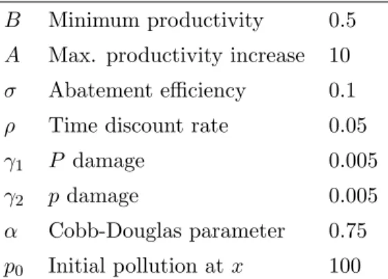
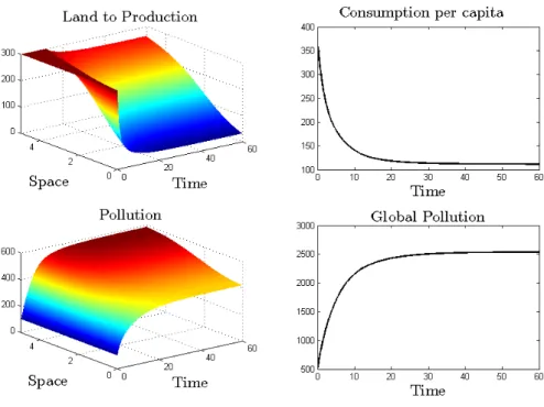
i.e., s(x) = 1 for all x. Figure 1 shows the results.

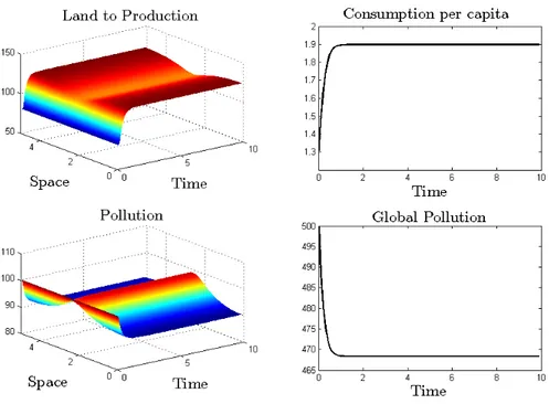
Figure 1: Benchmark scenario.

Given that there are no spatial disparities, it is not surprising that the optimal tra-jectories are uniform in space. The allocation of land to production starts at its highest possible level and remains unchanged until the environmental damage is large enough. At this point, land to production is optimally reduced and, consequently, the economy devotes part of the land endowment to abatement activities. Consumption shows a de-creasing trajectory due to the pollution damage of production and the replacement of

13_{We will consider the e↵ect of population agglomeration and the subsequent accrued need for housing}

land to production by abatement. Notice moreover that it eventually reaches a constant level, while local and global pollution continuously increases.

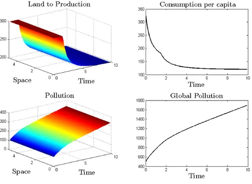
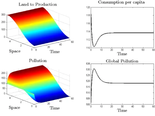
The optimal land trajectory attains a homogenous constant value too. Despite of using 2/3 of land to production, the economy cannot keep its initial level of consumption in the long-run due to the damage caused at the beginning. Both types of pollution cause indeed everlasting and increasing damage that the current abatement is not able to completely eliminate. However, if the efficiency of abatement is large enough our model shows that pollution can be stabilized. This outcome is illustrated in Figure 2, where the abatement efficiency parameter ( ) is equal to 0.9.

Figure 2: Pollution stabilization.

As we can see in this figure, the economy reaches a time-invariant solution. In contrast to Figure 1, (local and global) pollution becomes constant after some periods, together with consumption per capita and land to production. Consumption per capita, moreover, always increases during the transition, while a decreasing trajectory arises in the benchmark scenario due to the growing contamination. Notice also that in Figure 2 we have chosen a particularly high abatement efficiency (nine times the efficiency considered in Figure 1) in order to point out e↵ect pollution abatement. A direct consequence of this assumption is that pollution eventually disappears. Finally observe that, even if the focus of our simulations is the quality behavior of the economy, the substantially lower consumption per capita in Figure 2 can be explain be means of taking into account the planner’s concern about the pollution at the end of the planning

period. In the benchmark scenario, the welfare reduction due to the large amount of contamination left is compensated with a high levels of consumption. This compensation is not important though in scenarios where the pollution is very reduced such as in the scenario considered in Figure 2.

Let us study in the next sections the emergency of spatial patterns and the implica-tions of the di↵erent elements of our model in this regard.

5.2

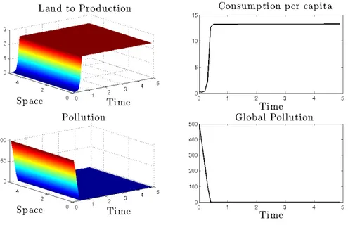
Role of abatement technology

We consider here a simple case of heterogeneous abatement technology in which abate-ment efficiency continuously deteriorates as we get afar from x = 0:14

(x) = 0.1 + 0.19

1 + ex 2.5.

This logistic form can be interpreted as a continuous representation of a step function, where some locations are better suited for abatement activities than others. In our

particular example the abatement efficiency parameter (x) monotonically decreases,

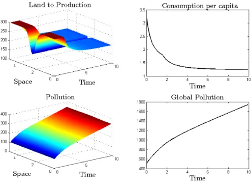
ranging from about 0.3 to 0.1. The results are displayed in Figure 3.

We can observe that the heterogeneity in abatement induces heterogeneity in land allocation from the beginning. Indeed at time t = 0, the less advanced locations in abatement specialise in production, whereas locations close to x = 0 focus on abatement. Due to this specialization, the areas devoted to production face greater levels of (local) pollution than the locations where abatement activities are intensified. Notice also that we have improved the abatement technology in all locations, with an efficiency that more than doubles for the most suited areas. As a result and in contrast to the benchmark case, locations compensate for emissions and the economy reaches a time-invariant solution. This outcome actually points out the role of abatement as pollution stabilizer. Moreover, in the same direction of Figure 2, pollution is reduced in areas where the abatement is sufficiently efficient.

Long-term consumption takes exactly the same value as in the benchmark, although consumption monotonically increases from the start as a direct consequence of the ac-crued abatement. Locations specialised in abatement produce little. This greater abate-ment e↵ort allows them to compensate for their relatively unimportant emissions and the

14_{For empirical evidence of di↵erences in abatement technology see, for instance, de Cara et al. (2005)}

Figure 3: Role of abatement technology.

incoming pollution from other locations that are better qualified for production activi-ties. However, regardless of locations’ production and/or abatement, the possibility of having consumption “imports”, as described in (3), enables homogeneous consumption and specialisation. Finally, since the time-invariant equilibrium is spatially heteroge-nous, we can also conclude that permanent di↵erences in abatement technology allow for lasting heterogeneity in land allocation and local pollution.

• Local and global damage

We have considered in the previous scenarios that both local and global pollution causes

the same damage per unit, i.e., 1 = 2. Consistently however with the examples

provided in sections 1 and 2, our model also allows us to study the case of contaminants with only local or only global e↵ects.15

When the damage is only local 1 is equal to zero in ⌦. Since in this case the damage

15_{The results of these scenarios are qualitatively equivalent to the case of pollutants with mainly}

local ( 2 > 1) or mainly global ( 2 < 1) e↵ect. Obviously, if 1 = 2 = 0 no land will be devoted

to abatement since pollution does not damage our economy. Therefore, consumption will stay at its maximum constant level (after taking housing into account, the remaining land will be completely assigned to production), where both local and global pollution increase steadily.

Figure 4: Damage function only depends on local pollution ( 1= 0).

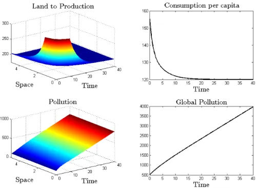
does not depend on global pollution, which is the largest pollutant by definition, the total damage of pollution is lower than in the previous scenario. As a consequence, one can see in Figure 4 that at first no location abates. Nevertheless, specialization emerges when the level of local pollution is high enough. The economy eventually reaches a time-invariant equilibrium, which is qualitatively identical to the previous case. However, the levels of local and global pollution are higher because of a lower damage of pollution. This result also points out that if the contamination damage is high enough (Figure 3) pollution will be optimally lower than when its damage is small (notice that local pollution is even reduced in some areas of the space in Figure 3). Parallel to the transition dynamics in figures 1 and 2, consumption per capita decreases until its time-invariant level, while this trajectory is increasing in Figure 3, where pollution is lower.

One should also observe that the rise of spatial heterogeneity is postponed until the economy accumulates enough contamination. This can also explain why consumption is initially higher than in the previous case: land devoted to production is higher and pollution damage is lower. We therefore conclude that, due to a lower pollution harm, the absence of global damage can delay the emergence of spatial patterns. This is an interesting dynamic property of our framework. Among the di↵erent scenarios that our simple set-up can reproduce, we can also include cases of delayed spatial heterogeneity.

From an economic perspective, this outcome points out the spatial-dynamic dimension of the problem. Even if there is spatial connectivity, the accumulation e↵ect (of pollution in our model) should be taken into account in order to fully understand how a particular element (abatement efficiency in this scenario) can induce spatial heterogeneity.

Let us consider the situation where the damage is only global ( 2 = 0). For our

parameters values, and among the two previous exercises, this situation corresponds to an intermediate case of pollution damage. On the one hand, Figure 3 represents the case where pollution has both local and global e↵ects, so the resulting damage is the highest. On the other hand, in Figure 4 the damage of pollution is the lowest because its e↵ect is only local. We can thus expect that the response of the economy when the damage is only local will be a combination of these two cases.

Figure 5: Damage function only depends on global pollution ( 2 = 0).

As it is clear from Figure 5, consumption and global pollution initially behave like in case of the lowest pollution damage, that is when pollution has only local e↵ects. The reason of this similarity is that pollution takes time to accumulate so that productivity losses are postponed, and the pollution damage is lower than in the case where pollu-tion has both local and global e↵ects. Still, in contrast to Figure 4, land specialisapollu-tion emerges from the beginning because (by definition) global pollution is always greater than the local one. Notice that, because the damage of pollution is lower, the

econ-omy produces and consumes more than in the case considered in Figure 3 despite the abatement specialization of part of the space.

Figure 5 also shows that consumption reduces in the starting periods. But later on, when pollution is large enough, the economy evolves like in the case where pollutions has both local and global e↵ects (see Figure 3). Since the locations specialised in abatement produce very little, pollution reduces in these areas, while it rises in the locations that focus on production. Nevertheless, even if its e↵ect is only global, pollution moves gradually in space until it reaches the areas devoted to abatement. Consequently, after some periods, local and global pollution stabilize, and consumption increases until its time-invariant level as in the case corresponding to Figure 3.

Just to conclude this section, let us point out two interesting features that the last numerical exercise reveals. First, one could believe that the global nature of pollution tends to homogenize space. Our example shows, however, that spatial heterogeneity can emerge even when pollution only has global e↵ects, due to pollution di↵usion and the spatial specificity of abatement activities. Second, in contrast to the previous two cases, pollution di↵usion can generate transitional dynamics that are non-monotonic (see Figure 5). This property underlines that, despite the simplicity of our model, we can provide scenarios with spatial heterogeneity and complex dynamics in time.

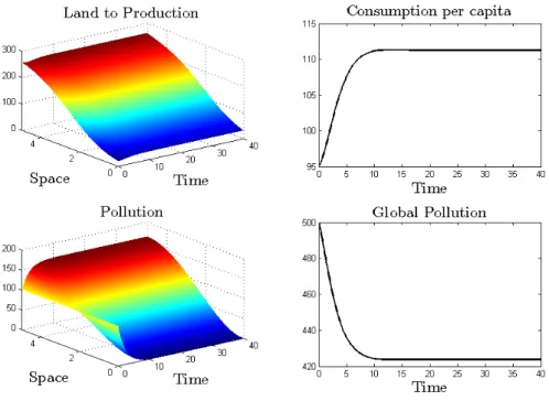
5.3

Spatially heterogeneous sensitivity to pollution

We consider the situation where some areas of the space are more sensitive to pollution than others. This case illustrates, for instance, the impact of pollution on global warming and the subsequent rise of the sea level. Many authors have recognized the importance of this negative e↵ect of pollution and, in particular, the associated degradation of soil quality (for instance, Nicholls and Cazenave, 2010). Similarly, the desertification of drylands gives us another example of spatial heterogeneity related to di↵erences on pol-lution sensibility (among others, Reynolds et al., 2007). In both cases, global warming is usually associated with the increase of global pollution such as the anthropogenic GHGs. In our simplified set-up, we can study this problem by means of assuming that the sen-sitivity to global pollution s(x) in the damage function ⌦ is spatially heterogenous. We specifically consider the following sensitivity function:

s(x) = 10 1 + e0.025 x 4 ⇣ 1 x 5 ⌘ .

As before, we consider a logistic function. But in this scenario locations are more sensi-tive to global pollution as they get afar from x = 0, with a sensitivity parameter ranging from about 1 to 10. Moreover, we assume greater concavity in order to emphasize the environmental sensitivity e↵ect (i.e., a relative large number of “fragile” locations). The numerical results are presented in Figure 6. We can observe that production is initially

Figure 6: Spatially heterogeneous sensitivity to pollution.

larger in less sensitive locations. Land devoted to production decreases indeed as one gets afar from x = 0. However, di↵erences in land allocation eventually vanish and the amount of land assigned to production reaches a constant spatially homogeneous level. This result goes against the a priori belief that the most sensitive regions would produce less than the others (and, consequently, “import” most of their consumption) in order to preserve their environmental quality. The explanation of this homogene-ity outcome is the following. Since pollution flows across locations, even the regions with non-existent or little production will experience positive levels of local pollution. Moreover, the pollution as a whole (global pollution) damages production too. Due to these two sources of pollution damage, the less sensitive locations optimally reduce their production, devoting as well land to abatement. If the most sensitive locations were endowed with better abatement technology they would then dedicate more land to abatement relatively to the less sensitive locations.

Let us finally point out that the numerical exercise considered in this section also illustrates an interesting spatial dynamic feature: an initial spatial heterogeneity (in land assigned to production, due to the spatial di↵erences in pollution sensitivity) can vanish in the long-run. In contrast to the previous scenarios, we are showing here that the di↵usion forces can also drive spatial homogeneity. Our numerical illustration actually presents an economy that eventually converges to the benchmark scenario, which is mainly characterized by its spatial homogeneity (see Figure 1).

5.4

The e↵ect of population agglomeration

Up to now our numerical exercises focused on the trade-o↵ between production and abatement. Accordingly, we have minimized in the previous sections the constraint of retaining some land for housing. As a last experiment, let us then analyse the e↵ect of population agglomeration and the resulting housing requirement. We consider in this regard that population is distributed following a Gaussian function over the interval [0, 5], that is, population agglomerates around the center of the space, x = 2.5. In order to underline the e↵ect of population agglomeration, we set total population to 10500 so that population in x = 2.5 is almost 130. Consequently, although the land endowment of each location is still equal to 300, in the central area of the space the proportion of L devoted to housing is much larger than in previous scenarios due to accrued population.16 _{This contrast with the locations far away from the center, where}

the weight of population is similar to that in the benchmark scenario.

Let us first compare the optimal trajectories under population agglomeration with the benchmark scenario. Figure 7 shows that, due to population concentration, locations in the central area cannot devote as much land to production as the locations at the far ends. This means that agglomerations optimally “import” most of their consumption from the neighbouring areas, which are more specialised in production. One could arguably think that agglomerations would be less locally polluted because most of the production comes from the periphery and housing does not involve emissions in our simplified framework. However, by the same token, agglomerations cannot devote as much land to abatement as the rest of locations. We thus observe a heterogeneous

16_{Notice that, in the previous scenarios, this increase in total population is sizable. However, a}

homogenous distribution of 10500 people over 500 locations would imply 21 individuals per location. In our simplified setup, 21 individuals would need 21 units of land for housing, which still is a small figure with respect to the land endowment of each location.

Figure 7: The role of population agglomeration (Gaussian distribution).

distribution of land to production, with almost no abatement in the center of the space. Consequently, local pollution in the central area is not lower than in other locations. We actually find that slight spatial disparities persist since agglomerations cannot abate pollution coming from neighbouring regions.17 _{This point is reinforced in the experiment}

considered in Figure 8.

In this second exercise we have doubled abatement efficiency in all locations (i.e., (x) = 0.2 for all x). In e↵ect, due to this technological improvement, all locations devote some land to abatement from the beginning. Both local and global pollution levels decrease then, allowing for a greater consumption per capita in the long-term. However, spatial disparities are amplified since the abatement capacity of the central area is constrained by its housing requirement.

We should finally observe that in this last scenario all variables reach a time-invariant solution, which is characterized by lasting spatial heterogeneity in both land allocation and local pollution. As in Section 5.2, this result points out again the role of abatement as pollution stabilizer. Abatement efficiency indeed enhances consumption and enables

17_{Pollution due to housing and/or transportation would amplify this e↵ect. These additional sources}

of contamination may have potential interesting implications, in particular if labour were a spatially mobile production factor.

Figure 8: Population agglomeration with abatement efficiency doubling.

the economy to reach a time-invariant equilibrium, which can be spatially heterogenous.

5.5

Further comments

Let us conclude the simulations of our paper with an additional discussion about the time-invariant solution and, in particular, its uniqueness as stated in Proposition 4. We will also complete the numerical analysis with a robustness check of the algorithm regarding the optimal trajectories.

In Section 3.2 we have studied the time-invariant equilibrium. As it is clear from the previous simulations, we have found several cases where the economy ends up in a time-invariant solution. Our algorithm actually provides a numerical tool to analyse the convergence to this kind of equilibrium. However, the multiplicity of this kind of long-term solution cannot be a priori ruled out. Still, in this regard, Proposition 4 in Section 3.2 turns out to be very useful since it allows us to identify a sufficient condition for uniqueness of time-invariant solutions. Since this condition was originally stated for the case when production is described by A⌦F , we must adapt it to the simulated case where production is given instead by ( ˜B + ˜A ˜⌦)F . Taking A⌦ = ( ˜B + ˜A ˜⌦), the condition

is rewritten as: ˜

⌦11(¯p, ¯P ), ˜⌦21(¯p, ¯P ) > 0 and ˜BF (¯l) + ˜AF (¯l)[ ˜⌦(¯p, ¯P ) p ˜¯⌦1(¯p, ¯P )] > G(1 f ¯l)

at every x. We can then apply it to our numerical illustrations. The condition is in fact verified in our simulations for every case where convergence towards a time-invariant interior solution is observed. Proposition 4 therefore ensures that this equilibrium is the unique time-invariant solution.

About the optimal paths, regardless the convergence to a time-invariant equilibrium, we should point out that the uniqueness property of the trajectories is still a mathe-matical open question. Therefore, since our problem may have more than one optimal solution, we may wonder to which extent the solutions presented in this section depend on the set of initial guesses. We have then performed several robustness checks in this respect. In these exercises we modify the initial guesses for the shadow price of pollu-tion, land devoted to producpollu-tion, and aggregated consumppollu-tion, in configurations with homogeneous or heterogenous distribution of population, abatement technology, and sensitivity to pollution. The results confirm that our algorithm is robust and always generates the same optimal trajectories.

More specifically, recall that in our numerical exercises the reversed-time shadow price of pollution{h0n

j }n=1...Nj=1...J was set to -5000. We have run simulations where{h0nj }n=1...Nj=1...J

ranges from 4750 to 100, leaving all else equal. We have similarly varied the initial guess for land to production from 25 to 250. Finally, we have considered in the sim-ulations that the initial guess for aggregated consumption was about 135. We so vary this value from 25 to 200. In all cases, the solution trajectories for local and global pollution, as well as for land distribution, coincide with those presented in the previous subsections. We thus conclude from these results that our algorithm is robust with respect to the initial guesses.18

6

Concluding remarks

The main objective of this paper is to present a benchmark framework to study optimal land use, encompassing land use activities and pollution. In our model, although land is immobile by nature, local actions a↵ect the whole space through pollution, which flows across locations resulting in both local and global damages. We find that our benchmark