HAL Id: hal-01523026
https://hal.inria.fr/hal-01523026
Submitted on 16 May 2017
HAL is a multi-disciplinary open access
archive for the deposit and dissemination of
sci-entific research documents, whether they are
pub-lished or not. The documents may come from
teaching and research institutions in France or
abroad, or from public or private research centers.
L’archive ouverte pluridisciplinaire HAL, est
destinée au dépôt et à la diffusion de documents
scientifiques de niveau recherche, publiés ou non,
émanant des établissements d’enseignement et de
recherche français ou étrangers, des laboratoires
publics ou privés.
A multidimensional brush for scatterplot data analytics
Michaël Aupetit, Nicolas Heulot, Jean-Daniel Fekete
To cite this version:
Michaël Aupetit, Nicolas Heulot, Jean-Daniel Fekete. A multidimensional brush for scatterplot data
analytics. IEEE. Visual Analytics Science and Technology (VAST), 2014 IEEE Conference on, Oct
2014, Paris, France. IEEE, pp.221 - 222, 2014, �10.1109/VAST.2014.7042500�. �hal-01523026�
A multidimensional brush for scatterplot data analytics
Michaël Aupetit1, Nicolas Heulot2, Jean-Daniel Fekete3
Abstract—Brushing is a fundamental interaction for visual analytics. A brush is usually defined as a closed region of the screen used to select data items and to highlight them in the current view and other linked views. Scatterplots are also standard ways to visualize values for two variables of a set of multidimensional data. We propose a technique to brush and interactively cluster multidimensional data navigating through a single of their scatterplot projection.
Index Terms—Visual analytics, brushing, scatterplot, multidimensional data, axis-parallel projection
IN TR O DU C T IO N
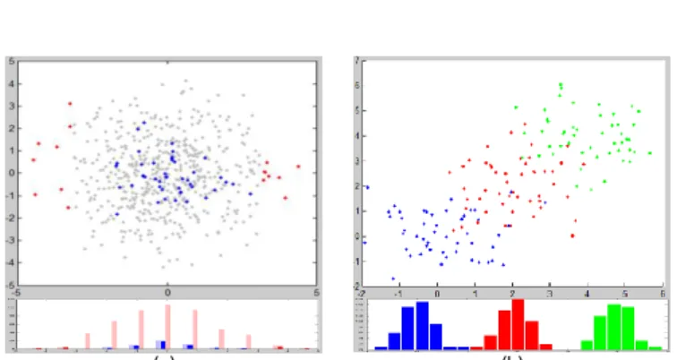
Brushing is a standard interaction technique for visual analytics. A brush is usually a closed region of the display used to select data items and to highlight them in the current view and other linked views. The reason for brushing data can be the focus on specific visual patterns like outliers or clusters in one view that the user wants to link to other views for further analysis. It is also a way to select data to be filtered out or to be highlighted permanently to keep track of detected patterns for future interactions. Clusters are important patterns in Exploratory Data Analysis. Data within a cluster are more similar to each other than to other data clusters. Two-dimensional (2D) scatterplots are also a standard way for data visualization where each data is represented as a point in a 2-dimensional Cartesian space. When data are multi2-dimensional (MD), 2D scatterplots can show an orthogonal projection of the data onto the plane formed by two of the data variables. However, this projection hides the MD cluster structure by possibly overlapping several distinct MD clusters in a single one. Even Scatter Plot Matrices (SPLOM) are unable to show this cluster structure for three possible reasons: the clusters are not pairwise linearly separable (Fig. 1a); the clusters are pairwise linearly separable but not by a hyperplane orthogonal to any one or two of the MD variables (Blue/red and red/green points in Fig. 1b); or the clusters are pairwise linearly separable by such a hyperplane but this is hidden by another cluster lying in between in any of the 2D scatterplots (Blue/green points separability hidden by the red points in Fig. 1b). In this work we focus on an interactive clustering task (a standard high-level analytic task in Exploratory Data Analysis) and define an MD brush which enables the user to solve these issues, exploring similarities between MD data through their 2D scatterplot, and to keep track of this exploration by coloring the MD clusters found.
1 MUL T I DIM EN SI O N AL B RU S H IN G
We consider a set P of D-dimension data x=(x1,…xD) as vectors in
the data space E=IRD , their orthogonal projection as a scatterplot of points (xa,xb) (a and b in {1,…,D}) in the 2D plane Eab and we define
a brush BS as a ball in S subspace of E with Euclidean radius rS and
center vS. In the sequel every distances and radius are Euclidean.
1.1 Brushing in 2D space
A standard brushing Bab(P) in the scatterplot Eab consists in selecting
points from P whose distance to vab=(va,vb) is lower or equal to rab.
The points selected are assigned a color or shape contrasting to non-selected points. The radius rab of this 2D-brush can be tuned with a
slider or the mouse wheel, while its center position vab can be
assigned to the mouse pointer position. This brush selects data points in the subspace Qab = Bab x E\a\b. The brush is local in Eab but not in
E\a\b (E = Eab x E\a\b) so it ignores any cluster structure in the E\a\b subspace as illustrated in Fig. 1.
(a) (b)
Fig. 1: 10D data scatterplot along two of their variables: (a) data from a 10D unit variance Normal (UVG) (grey and blue) centered within a 10D 5-unit radius sphere (grey and red); Below, histogram of the data, the ones within a 4-unit radius tube along the x-axis are highlighted. (b) data from three 10D UVG centered at (0,…,0); (2,…,2) and (4,…,4). Data histograms along the (0,…,0) to (1,…,1) diagonal. User task: clusters (colors) are unknown, they are to be discovered interactively.
1.2 Brushing in MD space
The multidimensional brush (MD-brush) is obtained by setting S=E, the MD-brush is then a D-dimension ball BE with radius rE centered
at some point v in E, that can be visualized as a disc Bab with radius
rab and center vab=(va,vb) in the scatterplot Eab. This Bab disc defines a
Magic Lens [1]: the appearance of the data points lying within this disc is altered based on the MD-brush selection process.
MD-brush selection: Data whose MD distance to vE is lower or equal
to rE are lying within the MD-brush. Among these points, only the
ones who also lie within the 2D magic lens are selected. We highlight these selected points by changing their shape (Fig. 2.). This highlighting in the scatterplot is linked to the current MD-brush selection and changes instantly with it.
MD-brush positioning: The mouse pointer position in Eab
corresponds to a whole D-2 subspace of E, so it cannot be used in general to set the HD position of the MD-brush center v. Therefore we propose to set v to the HD position of the nearest 2D data point to the mouse pointer.
Magic lens radius rab tuning: The radius of the magic lens can be
tuned using the mouse wheel. The smaller the radius, the more local the analysis of the MD cluster structure in the neighborhood of the MD-brush center v but the lower the number of points selected to get statistically relevant outcomes.
MD-brush radius rE tuning: The radius of the MD-brush is not
straight-forward to tune. Indeed, while it seems natural to set rE
equal to rab, the probability for BE to be empty while Bab is not would
increase with D. This is an effect of the curse of dimensionality [2]. If distances between data in Eab scale with unity on average, then
MD distances between data in E scale with the square root of D. Moreover if we consider a D-variate unit variance Normal distribution of data points centered at v, the distances of the data points to v follow a Chi distribution, so the smallest rE so that BE
captures all the points lying within Bab may be far larger than rab. 1 QCRI. [email protected]. 2 IRT SystemX.
We propose to support the user by visualizing as a bar graph, the distribution of the MD distances of any data points in Bab to the
center v of BE together with the Chi distribution of the distances of
points drawn from a D-variate Normal distribution centered at v with a diagonal covariance matrix whose non-zeros elements are all equal to ² =rab. The radius of the 95% quantile circle of a
bivariate unit variance Normal is equal to 2.45. So if MD data would come from a single D-variate Normal centered at v with variance ,
then their 2D projection in Eab would be also a Normal with center
vab and variance² so that the Magic Lens Bab would contain 95% of
the data. Thus this setting assumes the user selects a 2D cluster in Bab
and sees how the distances would be distributed if all of the data within the magic lens would represent the 95% core mass of a single D-variate Normal-distributed cluster. This allows the user to tune rE
so the empirical MD distance distribution within BE is similar to the
theoretical Chi distribution thus defined. If the empirical distribution appears to be denser than the theoretical one for smaller MD distances, that means points are even more concentrated or lie within a lower dimensional subspace clustered around v. We draw a vertical line indicating the 95th percentile of the Chi distribution which can be used as a default setting for rE (Fig. 2 and 3).
MD-brush clustering: A control key enables the user to permanently
color the selected points to keep track of MD clusters found. The interactive clustering process we propose is in the spirit of density-based automatic clustering approaches [3]. The user starts positioning the Magic Lens at some point in the scatterplot, then tunes the MD-brush radius rE to get a near Normal-cluster-like MD
distance distribution, then assigns the selected points to the current cluster and keeps up exploring the border of the current MD cluster point by point to enlarge or retract it. Notice that focusing the next MD-brush on a currently selected point in the 2D scatterplot corresponds to navigate continuously from a data point to its neighbours in the MD space E.
2 AN AL YT I C C AS E
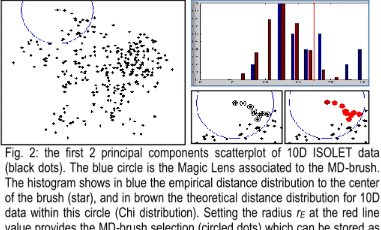
The data used for the experiment are letters ‘a’, ‘b’, ‘c’, ‘d’ and ‘e’ from the ISOLET dataset provided by the UCI machine learning repository. Each one of these letters were pronounced twice by 150 English speakers, 617 features were extracted from the signals. We kept the first 30 speakers for each letter so we got 300 instances of 617-dimension data that we further reduce to keep the 10 leading principal components using PCA. We attempted to extract manually the 5 clusters using the MD-brush through the scatterplot of the first two leading principal components. The basic interactive process of MD-brushing is demonstrated in Fig. 2, 3 and 4. At the end we got 3 clusters, one of which appeared to contains 3 of the original clusters (Fig. 4). We checked (Table 1) that these 3 clusters where not pairwise linearly separable in the 10D feature space, while they were all pairwise linearly separable with the two other clusters, supporting the correctness of the clusters we found with MD-brush.
Fig. 2: the first 2 principal components scatterplot of 10D ISOLET data (black dots). The blue circle is the Magic Lens associated to the MD-brush. The histogram shows in blue the empirical distance distribution to the center of the brush (star), and in brown the theoretical distance distribution for 10D data within this circle (Chi distribution). Setting the radius rE at the red line
value provides the MD-brush selection (circled dots) which can be stored as part of a cluster (red spots with dark red for the focused data point).
Fig. 3: After some MD-brush clustering (left), the circled dots and the blue spots are within the current MD-brush while yellow dots are not, therefore the circled dots will be added to the blue cluster. Later (right), a case where no clear cluster appears (no MD distance on the left of the red line), setting
rE to 40 shows that the center lies at the border of blue and red clusters. It
will be assigned arbitrarily to the blue one.
Fig. 4: Coming back to the small magenta cluster (left) it appears to be within the MD-brush with many data from the yellow cluster (yellow spots). The same is true for the small green cluster (not shown). Both will be finally assigned to the yellow one. The final MD-brush clustering result (center) and the true classes (right, with letters ‘a’,’b’,’c’,’d’,’e’ encoded as red, green, blue, magenta, and yellow colors respectively). The yellow MD-brush cluster is very close to the true blue class, the red one very close to the true red class, and the dark blue very close to the union of magenta, yellow and green true classes.
Table 1: true class pairwise linear separability of the ISOLET data.
3 DI SC USS I ON
We showed that an MD-brush can help to explore MD data through a single 2D scatter plot visualization, and recover MD cluster structures that other standard scatterplot-based visualization like SPLOM even equipped with brush and link, would fail to reveal. MD-brush relies only on the MD distances between the data points, so it could be used with other MDS-like projection but this has not been studied yet. Moreover, this work is to be complemented with a user-study to test how intuitive it is for non-expert users to recover MD clusters within various datasets and how the design could be improved for instance to display the distances’ histogram within the scatterplot. At last, a future work would be to study how MD-brush could be extended combined with SPLOM, to select the space E to be explored for subspace clustering.
RE FE RE NC ES
[1] Tominski, C.; Gladisch, S.; Kister, U.; Dachselt, R. & Schumann, H.: A Survey on Interactive Lenses in Visualization. EuroVis State-of-the-Art Reports, Eurographics Association, 2014.
[2] François, D. ;Wertz, V.; Verleysen, M.: About the locality of kernels in high-dimensional spaces . ASMDA 2005, International Symposium on Applied Stochastic Models and Data Analysis, pp. 238-245. Brest (France), 17-19 May 2005.
[3] Kriegel, H.-P.; Kröger, P.; Sander, J.; Zimek, A.: Density-based Clustering. WIREs Data Mining and Knowledge Discovery 1 (3): 231–240, 2011.