Credit Risk Analysis using Machine and Deep Learning models

(1)

HAL Id: halshs-01719983

https://halshs.archives-ouvertes.fr/halshs-01719983

Submitted on 28 Feb 2018

HAL is a multi-disciplinary open access archive for the deposit and dissemination of sci-entific research documents, whether they are pub-lished or not. The documents may come from

L’archive ouverte pluridisciplinaire HAL, est destinée au dépôt et à la diffusion de documents scientifiques de niveau recherche, publiés ou non, émanant des établissements d’enseignement et de

Credit Risk Analysis using Machine and Deep Learning

models

Peter Addo, Dominique Guegan, Bertrand Hassani

To cite this version:

Peter Addo, Dominique Guegan, Bertrand Hassani. Credit Risk Analysis using Machine and Deep Learning models. 2018. �halshs-01719983�

(2)

Documents de Travail du

Centre d’Economie de la Sorbonne

Credit Risk Analysis using Machine and Deep learning models

Peter Martey ADDO, Dominique GUEGAN, Bertrand HASSANI

(3)

Credit Risk Analysis using Machine and Deep learning

models

I

Peter Martey ADDOa,b,∗, Dominique GUEGANc,b, Bertrand HASSANId,b

a_{Data Scientist (Lead), Expert Synapses, SNCF Mobilite} b_{Associate Researcher, LabEx ReFi}

c_{University Paris 1 Pantheon Sorbonne, Ca’Foscari Unversity of Venezia, IPAG}

Business School

d_{VP, Chief Data Scientist, Capgemini Consulting}

Abstract

Due to the hyper technology associated to Big Data, data availability and computing power, most banks or lending financial institutions are renewing their business models. Credit risk predictions, monitoring, model reliability and effective loan processing are key to decision making and transparency. In this work, we build binary classifiers based on machine and deep learning models on real data in predicting loan default probability. The top 10 impor-tant features from these models are selected and then used in the modelling process to test the stability of binary classifiers by comparing performance on separate data. We observe that tree-based models are more stable than models based on multilayer artificial neural networks. This opens several questions relative to the intensive used of deep learning systems in the en-terprises.

Keywords: Credit risk, Financial regulation, Data Science, Bigdata, Deep

learning

I_{This work was achieved through the Laboratory of Excellence on Financial Regulation}

(LabEx ReFi) supported by PRES heSam under the reference ANR10LABX0095.

∗_{Corresponding author.}

Email addresses: pkaddo2000@gmail.com (Peter Martey ADDO), dominique.guegan@univ-paris1.fr (Dominique GUEGAN),

(4)

1. Introduction

The use of algorithms raises many ethical questions. Beyond the technical skills required to understand them, we are referring to the various discussions which occurred in the past few years regarding the use of personal data and all the problems related to Big Data, particularly the GDPR directive (GDPR (2016)) arriving May 25, 2018. During the year 2017, a public consultation (CNIL (2017)) on the use and the development of algorithms appeared, creat-ing many conferences and public meetcreat-ings in France on artificial intelligence. What is really the subject? People are afraid by the use of personal data and do not exactly understand the role of the algorithms due to the fear that they will have decisional power in place of people. These questions and the debates around these ideas are legitimate.

In this paper, we focus on the algorithms that are used to take these decisions. Algorithms are used in different domains with different objectives. For instance, they are used inside the enterprises to recruit persons, in line with the profile proposed. Algorithms can simplify the process, making it quicker, more fluid, etc. Nevertheless, algorithms are a set of codes with specific objectives to attain certain objectives. In the process of recruiting, it can introduce, for instance, discrimination or a specific profile, and then ”format” the persons working in the enterprise. It is the same in case of a loan provided or not provided by a bank to an enterprise, where the decision depends on the algorithm used. Thus, necessity must exist to understand these kinds of abuses and to find ways or advertisers to control the use of the algorithms. In another way, it seems impossible to impose an algorithm a priori. Indeed, in this paper, we illustrate the fact that there exist several algorithms that can be used in parallel to answer a question, for instance, to provide a loan to an enterprise. We observe that there exist several strategies to attain the objective we have: the choice of the variables (or features), the criteria and the algorithm that provides an answer to the question.

At the same time, the question of scrapping the data and their storage is a pre-requisite before using the algorithms. Some platforms are specialists in capturing data on the internet and their storage. Then the data are filtered; one important question concerns the filtering of the data: how to control them, how to avoid a manipulation of the data at this step, how to prevent data from locking in groups of profiles, for persons, enterprises, etc. The

(5)

choice of the data used is also a key point for the objective that people want to attain when they use Big Data.

Thus, concerning this new field, a need for transparency is necessary; it should be one that does not stand in the way of innovation in the field of algorithms, but can otherwise make progress. The terms associated with this field are ethics, transparency, knowledge and lisibility of the process. To contribute to these objectives, some political choices are necessary for the formation of the users and of the developers, the information concerning the limits of the algorithms with an adequate formation for the institutions that want to use them intensively and of the users to understand the framework. We can face some competition in that domain between the experts (de-velopers of codes, of nonparametric modelling behind this field of activities); also, we can, very quickly, be confronted with the use of supervised or un-supervised learning techniques and end up being subjected to the quarrels of the experts if one is not trained for these topics. An algorithm has no legal personality; thus, humans need to be at the end of the process to take a decision, and then they need to control the system they use.

Finally, in this paper, we try to highlight the most important points: the quality of the data, the transparency of the way in which the algorithms work, the choice of the parameters, the role of the variables (features) to avoid bias (cloning, filtering bubble, manipulation), the role of the evalua-tion criteria and the importance of the humans in terms of final decision.

The novelty of this paper is to address some specific questions we en-counter when we want to use Big Data and Algorithms. We focus mainly on the questions related to the use of the algorithms to solve or attain an objec-tive. Here, it is the possibility for a financial institution to provide a loan to a company. The bank that has to provide a loan needs to verify the safety of the enterprise. To decide, there exist several ways; one option is to use some models with specific information. The way in which the bank decides is not well known, but the use of classical linear models is well known in the banking sector. Thus, in the present exercise, we refer to the Lasso approach as a benchmark and we compare its fitting and decision rule based on the AUC as well as RMSE criteria with other non-parametric models classified as machine learning and deep learning in the recent literature. We retain six

(6)

approaches: a random forest model, a gradient boosting machine and four deep learning models. We specify the models and precise the choice done or retained (after optimisation procedures) for the parameters of each model. Besides the choice of the model, another question that arises concerns the choice of the variables (or features) to decide if an enterprise is eligible for a loan or not. We have used data provided by a European bank (thus, nothing is arbitrary in our further discussion) and we analyse the way in which the algorithms used or retained the variables.

This exercise exhibits three key points: the necessity to use (i) several models, (ii) several sets of data (making them change to quantify their im-pact), and, lastly, (iii) several criteria. We observe that the choices of the features are determinant as also the criteria: they permit to show the diffi-culty of getting a unique or ”exact” answer and the necessity of analysing all the results in details, or introducing new information before making any decision. One very important point is the fact that the deep learning model can provide very interesting results; in this exercise, this is probably because it does not retain the variables correctly and is not able to differentiate them in a robust way; but, is not that often the case? Finally, we find that tree-based algorithms have high performances on binary classification problems compared to the deep learning models considered in our analysis.

This paper is organised as follows: In Section two, a unified description of the algorithms we use is given. Section three discusses the criteria used to classify our results, and a discussion on imbalanced data sets is provided. The parameters and criteria used for each model is given in Section four with the results: we analyse how the algorithms are used to provide a loan to a company. We also analyse in details the choice of the features retained by each algorithm and their impact on the final results. Section five concludes. 2. A unified presentation of Models

We present, briefly, the models we use in our application. We make the presentation as uniform as possible to be able to specify, for each model, the different choices we are confronted in (i) parameters, (ii) stopping criteria, (iii) activation functions. References are provided for more details.

(7)

2.1. Elastic Net

The linear regression is a very well-known approach. It has several ex-tensions; one is the Lasso representation (Tibschirani (1996)) another one

includes the elastic net approach with a penalty term that is part l1 or l2,

(Zhou and Hastie (2005)).1 _{In their paper (Friedman et al. (2010)) describe}

algorithms for the carrying out of related-Lasso models: they propose fast algorithms for fitting generalised linear models with the elastic net penalty. This methodology can be useful for Big Data sets as soon as the algorithm is built to outperform execution speed. The regression modelling can be linear, logistic or multinomial. The objective is prediction and the minimisation of the predictions error, improving both the choice of the model and the esti-mation procedure.

Denoting Y as the response variable and X the predictors (centred and

standardised), and considering a data set (xi, yi), i = 1, · · · , N , the elastic

net approach solves the following problem, for a given λ:

minβ0,β[ 1 2N N X i=1 (yi− β0− xTi β) 2 + λPα(β)] (1)

where the elastic net penalty is determined by the value of α:

Pα(β) = (1 − α) 1 2kβk 2 l2+ α kβkl1 (2) Thus, Pα(β) = p X j=1 [1 2(1 − α)β 2 j + α|βj|]. (3)

Pα(β) is the elastic-net penalty term and is a compromise between the Ridge

regression (α = 0) and the Lasso penalty (α = 1): the constraint for

min-imization is that Pα(β) < t for some t. The parameter p is the number of

parameters. Historically, this method has been developed when p is very 1_{There exist a lot of other references concerning Lasso models; thus, this introduction}

does not consider all the problems that have been investigated concerning this model. We provide some more references noting that most of them have not the same objectives as ours. The reader can read with interest Fan and Li (2001), Zhou (2006) and Tibschirani (2011).

(8)

large compared to N . The Ridge method is known to shrink the coefficients of the correlated predictors towards each other, borrowing strength from each other. Lasso is indifferent to correlated predictors. Thus, the role of α is determinant: in the presence of the correlation, we expect α close to 1 (α = 1 − ε, for small ε). There also exists some link between λ and α.

Generally, a grid is considered for λ as soon as α is fixed. A lq (1 < q < 2)

penalty term could also be considered for prediction.

The algorithm also proposes a way to update the computation, optimis-ing the number of operations that are needed to be done. It is possible to associate a weight to each observation, which does not increase the computa-tional cost of the algorithm as long as the weights remain fixed. The previous approach works for several models:

• Linear regression: the response belongs to R. Thus, we use the model (1). In that case the parameter of interest is α, another set of

param-eters to be estimated are λ, βi. The existence of correlation must be

considered to verify if the values used for those parameters are efficient or not.

• Logistic regression: the response is binary (0 or 1). In that case the

logistic regression represents the conditional probabilities p(xi) through

a linear function of the predictors where p(xi) = P (Y = 1|xi) =

1

1+e−(β0+xiβi), then we solve

minβ0,β[ 1 N N X i=1

I(yi = 1)logp(xi) + I(yi = 0)log(1 − p(xi)) − λPα(β)].

(4) • Multinomial regression: the response has K > 2 possibilities. In that

case the conditional probability is2 _:

P (Y = l|x) = e −(β0l+xTβl) PK k=1e−(β0k+x T_β k) . (5)

(9)

For estimation, the parameter α has to be chosen first, then simple least squares estimates are use for linear regression, but a soft threshold is in-troduced to consider the penalty term, through the decrementation of the parameter λ using loops. In the case of logistic regression, a least square approach is also considered. In the case of the multinomial regression, con-straints are necessary for the use of the regularized maximum likelihood. In any case, the Newton algorithm is implement.

2.2. Random Forest modelling

Random forests are a scheme proposed by Breiman (2000, 2004) for build-ing a predictor ensemble with a set of decision trees that grow in randomly selected subspaces of data, Biau (2012), Ernst and Wehenkel (2006), and for a review Genuer et al. (2008). A random forest is a classifier consisting of

a collection of tree-structured classifiers rN(x, βk), k = 1, ... where the βk are

independent identically distributed random variables used to determine how the successive cuts are performed when building the individual trees. The accuracy of a random forest depends on the strength of the individual tree classifiers and of a measure of the dependence between them. For each input X, the procedure will be able to predict, with the optimal number of trees, the output value 1 or 0. A stopping criteria will be used to minimise the error of the prediction.

More precisely the random trees are constructed in the following way: all nodes of the trees are associated with rectangular cells such that at each step of the construction of the tree, the collection of the cells associated with

the leaves of the tree (external nodes) forms a partition of [0, 1]d. The roots

of the trees is [0, 1]d_{, (d ≤ N ). The procedure is repeated a great number}

of times: (i) at each node, a coordinate of the input is selected with the

j-th feature having a probability pj ∈ (0, 1) of being selected; (ii) at each

node, once the coordinate is selected, the split is at the midpoint of the cho-sen side. At each node, randomness is introduced by selecting, a small group of input features to split on, and choosing to cut the cell along the coordinate.

Each randomized output tree rN is the average over all the output

ob-servations yi for which the corresponding variables xj fall in the same cell of

(10)

random partition containing X, we obtain rN(X, β) = PN i=1yi1xj∈AN(X,β) PN i=11xj∈AN(X,β) 1LN where LN = PN

i=11xj∈AN(X,β) 6= 0. We take the expectation of the rN with

respect to the parameter β to obtain the estimate of the rN. In practice the

expectation is evaluated by Monte Carlo simulation, that is, by generating M (usually large) random trees, and taking the average of the individual

outcomes. The randomized variables βk, k > 1 are used to determine how

the successive cuts are performed when building the individual trees.

If X have uniform distribution on [0, 1]d, then the response of the model

is

Y =X

j∈S

βjxj+ ε,

where S is a non-empty subset of d features. With this model, we choose the following parameters: the number of trees and the stopping criteria (called threshold in the literature) used to choose among the most significant vari-ables. Depending on the context and the selection procedure, the informative

probability pj ∈ (0, 1) may obey certain constraints such as positiveness and

P

j∈Spj = 1. The number M of trees can be chosen. It is well known that

for randomised methods, the behaviour of prediction error is a monotically decreasing function of M; so, in principle, the higher the value of M, the better it is from the accuracy point of view. In practice, in our exercise, we

will fit the following non-parametric function fb on the variables to get the

response Y : Y = 1 B B X b=1 fb(X), (6)

where B is the number of trees, and a stopping criteria 10−p is used, for

which p has to be chosen.

2.3. A Gradient Boosting Machine

We now consider a more global approach for which the previous one can be considered as a special case. Using the previous notations, Y for outputs and X for different N input variables, we want to estimate a function f mapping X to Y , minimising the expected value of some specified loss function L(Y, f ).

(11)

This loss function L(Y, f ) can include squared error (Y −f )2_{/2, absolute error}

|Y − f |, for Y ∈ R1_{, negative binomial likelihood log(1 + e}−2Y f_{) when Y ∈}

(−1, 1), M-regression considering outliers L(Y, f ) = (Y −f )2/2 if |Y −f | < δ,

L(Y, f ) = δ(|Y − f | − δ/2) if |Y − f | > δ with δ a transition point, and logistic binomial log-likelihood: L(Y, f ) = log(1 + exp(−2Y f )). A general representation could be:

f (X, (βi, ai)1,...p) = p

X

i=1

βih(X, ai) (7)

where the function h(X, ai) is a parametric or a non parametric function of

the input X characterised by the parameters ai.

For estimation purpose, as soon as we work with a finite sample, the pa-rameter optimisation is obtained using a greedy stage wise approach solving:

(βl, al) = argminβ,a N X i=1 (L(yi, fl−1(xi) + βih(X, ai)1,...p)). (8) Thus fl= fl−1(X) + βlh(X, , al). (9)

The equations (8) and (9) are called boosting when y ∈ (−1, 1) and

L(Y, f ) is either an exponential loss function e−Y f or negative binomial

log-likelihood. The function h(X, a) is usually a classification tree. The smooth-ness constraint defined in (8) can be difficult to minimise and is replaced by a gradient boosting procedure (steepest-descent procedure) detailed in Fried-man (2001), or FriedFried-man et al. (2001).

2.4. Deep Learning

Neural networks (NN) have been around even longer, since early super-vised NNs were essentially variants of linear regression methods going back at least to the early 1800s. Thus, while learning, networks with numerous non-linear layers date back at least to 1965; also, explicit Deep Learning (DL) research results have been published at least since 1991. The expres-sion ”Deep Learning” was actually coined around 2006, when unsupervised pre-training of deep learning appeared through gradient enhancements and

(12)

automatic learning rate adjustments during the stochastic gradient descent. A standard neural network consists of many simple, connected processors called neurons, each producing a sequence of real-valued activations. In-put neurons get activated through sensors perceiving the environment; other neurons get activated through weighted connections from previously active neurons. An efficient gradient descent method for teacher-based supervised learning in discrete, differentiable networks of arbitrary depth, called back-propagation, was developed in the 1960s and 1970s, and applied to NNs in 1981. DL became practically feasible to some extent through the help of unsupervised learning. The 1990s and 2000s also saw many improvements of purely supervised DL. In the new millennium, deep NNs have finally at-tracted wide-spread attention, mainly by outperforming alternative machine learning methods such as kernel machines (Vapnik (1995); Scholkopf et al. (1998)) in numerous important applications. Deep NNs have become rele-vant for the more general field of reinforcement learning where there is no supervising teacher.

Deep Learning approaches consist in adding multiple layers to a neural network though these layers can take be repeated. Discussing the matter, most deep learning strategies rely on the following 4 types of architectures: (i) Convolutional Neural Networks, which, in essence, are standard neural networks that have been extended across space using shared weights; (ii) Recurrent Neural Networks, which are standard neural networks that have been extended across time by having edges that feed into the next time step instead of into the next layer in the same time step; (iii) Recursive Neural Networks, which are apparented to hierarchical networks where there is no time aspect to the input sequence but inputs have to be processed hierarchi-cally as in a tree. (iv) Finally, Standard Deep Neural Networks, which are a combination of layers of different types without any repetition or particular order. This is this last type that has been implemented in this paper.

In all these approaches, several specific techniques that we do not de-tail here are used. They concern (i) Back-propagation, which is a method to compute the partial derivatives, i.e. the gradient of a function. In this paper, we use the stochastic gradient descent, which is a stochastic approximation of the gradient descent optimisation and iterative method for minimising an objective function that is written as a sum of differentiable functions.

(13)

Adapting the learning rate for the stochastic gradient descent optimisation procedure can increase performance and reduce training time. The simplest and perhaps most used adaptations of learning rate during training are tech-niques that reduce the learning rate over time. (ii) Regularisation in deep learning: the approach consists of randomly dropping units (along with their connections) from the neural network during training. This prevents units from co-adapting too much. During training, dropout has been shown to improve the performance of neural networks on supervised learning tasks in vision, speech recognition, document classification and computational biol-ogy, obtaining state-of-the-art results on many benchmark datasets. It has shown no interest in our exercise. (iii) Dimensionality reduction is usually necessary for implementing Deep learning strategies. Max pooling can be used for this objective. It was not pertinent in our exercise. There exists numerous references on all these fields, some among others are, Siegelmann and Sontag, (1991), Balzer (1985), Deville and Lau (1994), and Hinton and Salakhutdinov (2006). For a complete and recent review we refer to Schmid-huber (2014).

The NNs behaviour or program is determined by a set of real-valued

pa-rameters or weights βj. To represent it in a uniform way, we focus on a single

finite episode or epoch of information processing and activation spreading, without learning through weight changes. During an episode, there is a

par-tially causal sequence xj, j = 1, ..., N of real values called events. Each xj

is an input, or the activation of a unit that may directly depend on other

xi, i < j through the current NN. Let the function f encoding information

and map events to weight indexes. The function f is any nonlinear function. Thus a classical NN layer performs a convolution on a given sequence X, outputting another sequence Y whose value at time t is as follows:

y(t) =

N

X

j=1

f (βj, xj(t)) + ε(t)

where βj are the parameters of the layer trained by backpropagation. In our

exercise, backpropagation is used, but also hierarchical representation learn-ing, weight pattern replication and sub-sampling mechanisms. We make use of the gradient descent method for optimisation convergence. The parame-ters we can choose are the number of layers, the stopping criteria. In case of an unsupervised deep learning system, regularisation functions are added

(14)

as activation functions. We specify them when we analyse the data sets and the results.

3. The criteria

There are several performance measures to compare the performance of the models including AUC, Gini, logLost function, RMSE and AIC; and we can use different metrics like the F-score, the recall and the precision. In this paper, we will put more emphasis on the AUC and RMSE criteria.

The Gini index was introduced by Gastwirth (1972) and extended by Yitzhaki (1983) and Lerman and Yitzhaki (1984). This index, in its essence,

permits to compare several algorithms. It is based on the decision tree

methodology and entropy measure. Raileanu and Stoffel (2004) discussed the possibility to compare algorithms using classification systems. From the empirical point of view, this problem has been discussed a lot. It seems that no feature selection rule is consistently superior to another and that Gini can be used to compare the algorithms; nevertheless, we will not use it in the paper, focussing on the ROC curve whose interpretation in terms of risks is

more efficient3.

For each company, we build the ROC curve. An ROC curve is then used to evaluate the quality of the model. The ROC approach can be often asso-ciated with the computation of an error from a statistical point of view. We now specify this point. If we want to associate the AUC value (coming from the ROC building) to Type I and Type II errors, we need to specify the test we consider and, thus, to determine the hypotheses, the statistics, the level and the power of the test. In our case the objective is to know if a bank can provide a loan to the enterprise, in the sense that the enterprise will not default. To answer this question, we use several models or algorithms and the idea is to find the algorithm which permits to answer this question with accuracy. The AUC criteria are used to do it; here, we explain why. To analyse, in a robust way, the results obtained with this indicator, we specify the risks associated with it. When a bank provides a loan to an enterprise, it 3_{As soon as AUC is known, the Gini index can be obtained under specific assumptions}

(15)

faces two types of errors: (1) to refuse a loan to a company whose probability of default is much lower than the one obtained with the model (Type I error); (2) to agree to provide a loan to a company whose probability of default is much higher than the value obtained with the selected model (Type II er-ror). We want these two errors to be as small as possible. We compute the probability of the corresponding events under the null and the alternative is that we specify these assumptions. We assume that a bank provides a loan

and the null is H0 : the company can reimburse the loan , α= P[the bank

does not provide a loan | the company can reimburse it] = PH0[the bank does

not provide a loan]: this is the Type I error; thus the alternative is H1 : the

company does not reimburse the loan, and β=P[the bank provides a loan |

the company cannot pay it back]= PH1[the bank provides a loan], this is the

Type II error.

Considering the data set, we are interested in the answer: the bank pro-vides a loan as the probability of default of the target company is sufficiently low (the model outcome has the value 1) or the bank does not provide a loan as the probability of default of the target company is not low enough (the outcome is now 0). These outcomes, 1 or 0, depend on a lot of variables that we use to compute the risks α or β. Note that to build the ROC curve, we make α varying (it is not fixed as it is in a general context of statistical test). When we build the ROC, on the x-axis, we represent 1 − α, also called

speci-ficity (in some literature). We want this number close to 14_{. On the y-axis}

we represent 1 − β, which corresponds to the power of the test and we want

that it is close to one. It is usually referred to as sensitivity5_{. In practice,}

when the ROC curve is built, all the codes are done under almost two kinds of assumptions on the data: the data are independent and the distribution under the null and the alternative are Gaussian; these assumptions can be far from reality in most cases. From the ROC curve, an index is built; it is the AUC. The AUC represents the area under the curve. How can we interpret its value? If the curve corresponds to the diagonal, then the AUC is equal to 0.5; we have one chance over two to make a mistake. If the curve is above the diagonal, the value will be superior at 0.5, and if it attains the horizontal at one, for all (1 − α), 1 is obtained which is the optimal value. Thus, as soon

4_{In medicine it corresponds to the probability of the true negative} 5_{In medicine corresponding to the probability of the true positive}

(16)

as the AUC value increases from 0.5 to 1, this means that we have less and less chance to make a mistake, whatever the value of (1 − α) between 0 and 1 (which means that the Type I error diminishes). We consider in fact that the test becomes more and more powerful because the probability for the bank to provide a loan and that the enterprise does not default is very high. Each algorithm provides a value of AUC. To be able to compare the results between the algorithms, we need to verify that we use the same variables to get the outputs 1 or 0. If that is not the case, the comparison will be difficult and could be biased.

Another question affects the quality of the results: it concerns imbal-anced data. The presence of a strong imbalance in the distribution of the response (which is the case for our exercise) creates a bias in the results and weaks the estimation procedure and accuracy of the evaluation of the results. A data set is imbalanced if the classification categories are not ap-proximately equally represented. Examples of imbalanced data sets have been encountered in a lot of fields, some references are Mladenic and Gro-belnik (1999) or Kubat et al. (1999) among others. Several approaches are used to create balanced data sets, either by over-sampling the minority class and under-sampling the majority class (Kubat and Marvin (1999) or Ling and Li (1998)); diverse forms of over-sampling can be used such as the one developed by Chawla et al. (2002). In this paper, the latter methodology has been implemented, blending under-sampling of the majority class with a spe-cial form of over-sampling the minority class associated with a naive Bayes classifier, improving the re-sampling, modifying the loss ratio and class prior approaches.

The approach, we use, proposes an over-sampling approach in which the minority class is over-sampled by creating ”synthetic” examples rather than by over-sampling with replacement. The synthetic examples are generated by operating in ”feature space” rather than in ”data space”. The minority class is over-sampled by taking each minority class sample and introducing synthetic examples along the line segments joining any/all the k minority class neighbours randomly chosen. To generate the synthetic examples, we proceed on the following path: we take the difference between the feature vector under consideration and its nearest neighbour. We multiply this dif-ference by a random number between 0 and 1 and add it to the feature vector under consideration. This causes the selection of a random point along the

(17)

line segment between two specific features. This approach effectively forces the decision region of the minority class to become more general. The major-ity class is under-sampled by randomly removing samples from the majormajor-ity class population until the minority class becomes some specified percentage of the majority class. This forces the learner to experience varying degrees of under-sampling; and at higher degrees of under-sampling, the minority class has a large presence in the training set. In our exercise, the rare events, n, correspond to less than 2% of the whole sample N (n= 1731, and N=117019).

4. Data and models

In this section6_{, we provide an overview of the data structure, models and}

then present results of model performance. 4.1. The Data

The information set contains 117019 lines, each of them representing ei-ther a default or not a default (binary value) of an enterprise when they ask for a loan from a bank. Default and good health are characterised by the same 235 labelled variables that are directly obtained from the companies: financial statements, balance sheets, income statements and cash flows state-ments where the values are considered at the lowest level of granularity. In the year 2016/2017, 115288 lines represented companies in good health and 1731 represented companies in default. Because of the bias created by imbal-anced data, in this exercise, we provide only results with balimbal-anced training data of the binary classes, following the method recalled in Section 3.

After importing the data, we clean them: this concerns the variables. We remove features with no pertinent information (same value for all the enterprises; sign with no available entries like NaN for instance). It remains 181 variables. Then we split the data in three subsets, considering 80% of the data (60% for the fitting and 20% for the cross validation) and then 20% of this data used for test purposes. The validation performance permits to 6_{Code implementation in this section were done in ’R’. The principal package used}

is H2o.ai (Arno (2015)). The codes for replication and implementation are available on https://github.com/brainy749/CreditRiskPaper

(18)

improve the training approach and we use it to provide predictions perfor-mance on the test set. In the training set, we verify if it is a balanced data set or not. Here it is: the value 0 represents 98,5% and the value 1, 1,5%. So, the extreme events are less than 2%. Using the Smote algorithm described in the previous Section, we obtain a balanced set with 46% of 0 and 53% of 1.

4.2. The models

The models we use have been detailed in the previous section. We focus on seven models: a logistic ridge regression, a random forest, a gradient boosting modelling and a neural network approach with four different complexities. To rank the models with respect to the companies’ credit worthiness, the ROC curve and AUC criteria as RMSE criteria are used. An analysis of the main variables is provided: first we use the 181 variables (54 variables have been removed); then we use the 10 first variables selected by each model, comparing their performance with respect to the models we use. An analysis on these variables completes the study.

4.2.1. Precisions on the parameters used to calibrate the models

To have a benchmark for comparison and replication of results, a fix seed is set. The models have been fitted using the balanced training data set.

• The Logistic regression model M1: to fit the logistic regression model-ing, we use the elastic net logistic regression and regularization func-tions. This means that the parameter in equations (2.1) and (2.2) can change. In our exercise, α = 0.5 in (2.3) (the fitting with α = 0.7

pro-vides the same results), and λ = 1.9210−6 (this very small value means

that we have privileged the ridge modelling) are used.

• The random forest model M2: using the equation (6) to model the random forest approach we choose the number of trees B = 120 (this choice permits to test the total number of features), the stopping

crite-rion is equal to 10−3 . If the process converges quicker than expected,

the algorithms stops and we use a smallest number of trees.

• The gradient Boosting model M3: to fit this algorithm, we use the logistic binomial log-likelihood function: L(y, f ) = log(1 + exp(−2yf )),

(19)

We need a learning rate which is equal to 0.3. At each step we use a sample rate which corresponds to 70% of the training set used to fit each tree.

• Deep learning: four versions of the deep learning neural networks mod-els with stochastic gradient descent have been tested.

1. D1: For this models 2 hidden layers have been implemented (this is motivated by the fact that we analyse binary data), and 120 neurons. This number depends on the number of features and we take 2/3 of this number. It corresponds also to the number used a priori with the random forest model and gives us a more comfortable design for comparing the results.

2. D2: Three hidden layers have been used, each composed of 40

neurons and a stopping criteria equal to 10−3 has been added.

3. D3: 3 hidden layers with 120 neurons each have been tested. A

stopping criteria equal to 10−3 and `1 and `2 regularization

func-tions have been used.

4. D4: Given that there are a lot of parameters that can impact model’s accuracy, hyper-parameter tuning is especially important for deep learning. So, in this model, a grid of hyper-parameters has been specified and then select the best model. The hyper parameters include the drop out ratio, the activation functions,

the `1 and `2 regularization functions, the hidden layers. We also

use a stopping criterion. The best model’s parameters yields a

dropout ratio of 0, `1 = 6, 8.10−5, `2 = 6, 4.10−5, hidden layers =

[50, 50], activation function is the rectifier (f (x) = 0 if x < 0, if not f (x) = x).

4.2.2. Results

Using 181 features, the seven models (M1 corresponding to the logistic regression, M2 to the random forest, M3 to the boosting approach and D1, D2, D3 and D4 for the different deep learning models) provide the ROC curve with the AUC criteria, and we also compute the RMSE criteria for each model.

Analysing Tables 1 and 2 using 181 variables, we observe that there exists a certain competition between the approaches relying on the random forest

(20)

Models AUC RMSE M1 0.842937 0.247955 M2 0.993271 0.097403 M3 0.994206 0.041999 D1 0.902242 0.120964 D2 0.812946 0.124695 D3 0.979357 0.320543 D4 0.877501 0.121133

Table 1: Models’ Performances on validation dataset with 181 variables using AUC and RMSE values for the seven models.

Models AUC RMSE

M1 0.876280 0.245231 M2 0.993066 0.096683 M3 0.994803 0.044277 D1 0.904914 0.114487 D2 0.841172 0.116625 D3 0.975266 0.323504 D4 0.897737 0.113269

Table 2: Models’ Performances on test dataset with 181 variables using AUC and RMSE values for the seven models.

(21)

(M2) and the one relying on gradient boosting (M3). The interesting point is that the complex deep learning in which we have tried to maximise the use of optimisation functions does not provide the best models.

On the validation set, we observe that the AUC criteria have the highest value with the model M3, then the model M2, then D3, and for the four last places, the model D1, then D4, M1 and D2. If we consider the RMSE criteria, the model M3 provides the smallest error, then the model M2, then D1 and D4, and finally, D2, M1 and D3. Thus, the model D3 has the highest error. We observe that the ranking of the performance metric is not the same using the AUC and RMSE criteria.

On the test set, we observe the same ranking for AUC and for RMSE as with the training set, except for D1 and D4 that switch between the third and the fourth place. D3 provides the highest AUC among the deep learning models; however, it yields the highest error.

If the gradient boosting model remains the best fit (using the AUC) with the smallest error, we observe stability of models on both validation and test sets. In all scenarios, we observe that the deep learning models do not outperform the tree-based models (M2, M3). The comparison between the results obtained with AUC criteria and the RMSE criteria indicate that a unique criterion is not sufficient.

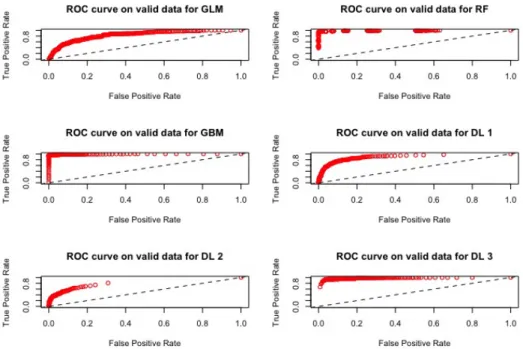
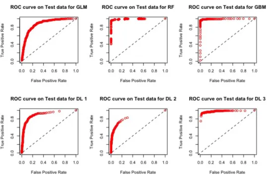
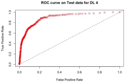
The ROC curves corresponding to these results are provided in the Fig-ures 1 - 4: they illustrate the speed at which the ROC curve attains the value 1 on the y-axis with respect to the value of the specificity. The best curve can be observed on the second row first column for the validation set on Figure 1 and for the test on Figure 3: it corresponds to the model M3.

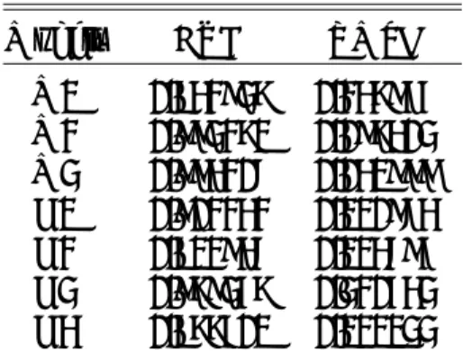
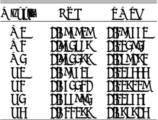
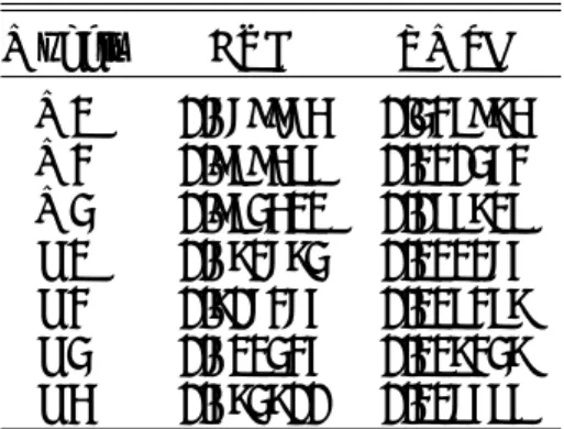
Each model M1-M3 and D1-D4 has used the same 181 variables for fit-tings. In terms of variable importance, we do not obtain the same top ten variables for all the models, Gedeon (1997). The top ten variables’ impor-tance for the models are presented in Table 3: they correspond to 57 different

variables. We refer to them as A1, ...A57(they represent a subset of the

orig-inal variables (X1, . . . , X181). Some variables are used by several algorithms,

(22)

Figure 1: ROC curves for the models M1, M2, M3, D1, D2, D3 using 181 variables using the validation set.

M1 M2 M3 D1 D2 D3 D4

X1 A1 A11 A11 A25 A11 A41 A50

X2 A2 A5 A6 A6 A32 A42 A7

X3 A3 A2 A17 A 26 A33 A43 A51

X4 A4 A1 A18 A27 A34 A25 A52

X5 A5 A9 A19 A7 A35 A44 A53

X6 A6 A12 A20 A28 A36 A45 A54

X7 A7 A13 A21 A29 A37 A46 A55

X8 A8 A14 A22 A1 A38 A47 A56

X9 A9 A15 A23 A30 A39 A48 A57

X10 A10 A16 A24 A31 A40 A49 A44

(23)

Figure 2: ROC curve for the model D4 using 181 variables using the validation set.

We now investigate the performance of these algorithms using only the ten variables selected by each algorithm. We do this work for the seven mod-els. The results for the criteria AUC and RMSE are provided in Table 10. The results obtained with the test set are only provided.

For all the tables, we get similar results. The M2 and M3 models perform significantly compared to the five other models, in terms of AUC. The deep learning models and the based logistic model poorly perform on these new data sets. Now, looking at the RMSE for the two best models, M3 is the best in all cases. The highest AUC and lowest RMSE among the seven models on these data sets is provided by the M3 model using the M3 top variables (Table 6).

Comparing the results provided by the best model using only the 10 top variables with the model fitted using the whole variables set (181 variables), we observe that the M3 model is the best in terms of highest AUC and small-est RMSE. The tree-base models provide stable results, whatever the number of variables used, which is not the case when we fit the deep learning models. Indeed, if we look at their performance when they use their top ten variables, this one is very poor: refer to line four in Table 7, line five in Table 8, line

(24)

Figure 3: ROC curves for the models M1, M2, M3, D1, D2, D3 using 181 variables with the test set.

six in Table 9, and line seven in Table 10.

Models AUC RMSE

M1 0.638738 0.296555 M2 0.98458 0.152238 M3 0.975619 0.132364 D1 0.660371 0.117126 D2 0.707802 0.119424 D3 0.640448 0.117151 D4 0.661925 0.117167

Table 4: Performance for the seven models using the Top 10 features from model M1 on Test dataset.

(25)

Models AUC RMSE

M1 0.667479 0.311934 M2 0.988521 0.101909 M3 0.992349 0.077407 D1 0.732356 0.137137 D2 0.701672 0.116130 D3 0.621228 0.122152 D4 0.726558 0.120833

Models AUC RMSE

M1 0.669498 0.308062 M2 0.981920 0.131938 M3 0.981107 0.083457 D1 0.647392 0.119056 D2 0.667277 0.116790 D3 0.6074986 0.116886 D4 0.661554 0.116312

Table 7: Performance for the seven models using the Top 10 features from model D1 on Test dataset.

(26)

Models AUC RMSE

M1 0.640431 0.459820 M2 0.980599 0.179471 M3 0.985183 0.112334 D1 0.712025 0.158077 D2 0.838344 0.120950 D3 0.753037 0.117660 D4 0.711824 0.814445

Models AUC RMSE

M1 0.650105 0.396886 M2 0.985096 0.128967 M3 0.984594 0.089097 D1 0.668186 0.116838 D2 0.827911 0.401133 D3 0.763055 0.205981 D4 0.698505 0.118343

(27)

Figure 4: ROC curve for the model D4 using 181 variables with the test set.

in terms of AUC and RMSE the logistic regression model (M1) and the multi-layer neural network models (deep learning D1-D4)) considered in this study in both the validation and test datasets using all the 181 features. We ob-serve that Gradient Boosting model (M3) demonstrates high performance for the binary classification problem compared to Random Forest model (M2), given lower RMSE values.

Upon selection of the top 10 variables from each model to be used for modelling, we obtain same conclusion of higher performance with models M2 and M3, with M3 as the best classifier in terms of both AUC and RMSE. The Gradient Boosting model (M3) recorded the highest performance on test dataset on the top 10 variables selected, out of 181 variables by this model M3.

Now we look at the profile of the top 10 variables selected by each model.

We denote Ai, i = 1, · · · A57, the variables chosen by the models among the

181 original variables; we refer to Table 3. For instance, M2 selects 3 variables already provided by model M1. Model M3 selects only one variable provided by M1. The model D1 uses three variables of model M1. The model D2 selects one variable selected by model M2. Model D3 selects one variable

(28)

used by model D1. The model D4 selects one variable selected by M1. The classification of the variables used by each model is as follows: the

variables A1, ..., A10of the model M1 correspond to flow data and aggregated

balance sheets (assets and liabilities). It concerns financial statement data. The model M2 selects financial statement data and detail financial state-ments (equities and debt). The model M3 selects detail financial statestate-ments (equities and debt). The model D1 selects financial statement data and a lowest level of granularity of financial statement data (long term bank debt). The models D2 and D3 select an even lower level of granularity of financial statement data (short term bank debt and leasing). The model D4 has se-lected the most granular data, for instance, the ratio between elements as the financial statements.

Thus, we observe an important difference in the way the models select and work with the data they consider provided for scoring a company and as a result accepting to provide them with a loan. The model M1 selects more global and aggregated financial variables. The models M2 and M3 select detailed financial variables. The models relying on deep learning select more granular financial variables, which provide more detailed information on the customer. There is no appropriate discrimination among the deep learning models of selected variables and associated performance on test set. It appears that the model M3 is capable of distinguishing the information provided by the data and only retains the information that improves the fit of the model. The tree-based models, M2 and M3, turn out to be best and stable binary classifiers as they properly create split directions, thus keeping only the efficient information. From an economic stand point, the profile of the selected top 10 variables from the M3 model will be essential in deciding whether to provide a loan or not.

5. Conclusion

The rise of Big Data and data science approaches, such as machine Learn-ing and deep learnLearn-ing models, do have a significant role in credit risk mod-elling. In this exercise, we have showed that it is important to make checks on data quality (in the preparation and cleaning process to omit redundant variables) and it is important to deal with an imbalanced train dataset to

(29)

avoid bias to a majority class.

In this exercise, we show that the choice of the features to respond to a business objective (in our case, should a loan be awarded to an enter-prise? Can we use few variables to save time in this decision making?) and the choice of the algorithm used to take the decision (whether the enter-prise makes defaults) are two important keys in the decision management processing when issuing a loan (here, the bank). These decisions can have an important impact on the real economy or the social world; thus, regular and frequent training of employees in this new field is crucial to be able to adapt to and properly use these new techniques. As such, it is important that regulators and policy makers take quick decisions to regulate the use of data science techniques to boost performance, avoid discrimination in terms of wrong decisions proposed by algorithms and to understand the limits of some of these algorithms.

Additionally, we have shown that it is important to consider a pool of models that match the data and business problem. This is clearly deduced looking at the difference in performance metrics. Data Experts or Data Sci-entist need to have knowledge of model structures (in terms of choice of hyper-parameters, estimation, convergence criteria, performance metrics) in the modelling process. We recommend that performance metrics should not be only limited to one criteria like AUC. It is important to note that stan-dard criteria like AIC, BIC, R2 are not always suitable for the comparison of model performance, given the types of model classes (regression-based, classification-based, etc.). In this exercise, we noticed that the use of more hyper-parameters, as in the grid deep learning model, does not outperform tree-based models on the test dataset. Thus, practitioners need to be very skilled in modelling techniques and careful while using some black-box tools. We have shown that the selection of the 10 top variables, based on the variable importance of models, does not necessary yield stable results given the underlying model. Our strategy of re-checking model performance on these top variables can help data experts to validate the choice of models and variables selected. In practice, requesting for few lists of variables from clients can help speed up the time to deliver a decision on load request.

(30)

necessary provide the best performance and that regulators need to also ensure transparency of decision algorithms to avoid discrimination and a possible negative impact in the industry.

References

Arno, C., 2015. The definitive performance tuning guide for h2o deep learn-ing. H2O.ai, Inc.

Balzer, R., Nov. 1985. A 15 year perspective on automatic programming. IEEE Trans. Softw. Eng. 11 (11), 1257–1268.

URL http://dx.doi.org/10.1109/TSE.1985.231877

Biau, G., Apr. 2012. Analysis of a random forests model. J. Mach. Learn. Res. 13 (1), 1063–1095.

URL http://dl.acm.org/citation.cfm?id=2503308.2343682

Breiman, L., 2000. Some infinity theory for predictors ensembles. Technical Report, UC Berkeley, US 577.

Breiman, L., 2004. Consistency for a sample model of random forests. Tech-nical Report 670, UC Berkeley, US 670.

Chawla, N., Bowyer, K., Hall, L., Kegelmeyer, W., 2002. Smote:synthetic mi-nority over-sampling technique. Journal of artificial Intelligence Research 16, 321–357.

CNIL, Sep 2017. La loi pour une r´epublique num´erique. concertation

citoyenne sur les enjeux ´ethiques lies `a la place des algorithmes dans notre

vie quotidienne. CNIL Montpellier.

Deville, Y., Lau, K. K., 1994. Logic program synthesis. Journal of Logic Programming 19 (20), 321–350.

Ernst, D., Wehenkel, L., 2006. Extremely randomized trees. Machine learning 63, 3–42.

Fan, J., Li, R., 2001. Variable selection via nonconcave penalized likelihood and its oracle properties. Journal of the American Statistical Society 96, 1348 – 1360.

(31)

Friedman, J., Hastie, T., Tibshirani, R., 2001. The elements of statistical learning. Springer series in statistics 1, 337–387.

Friedman, J., Hastie, T., Tibshirani, R., 2010. Regularization paths for gen-eralized linear models via coordinate descent.

Friedman, J. H., 2001. Greedy function approximation: A gradient boosting machine. The Annals of Statistics 29 (5), 1189–1232.

Gastwirth, 1972. The estimation of the lorenz curve and the gini index. The review of Economics and Statistics, 306 – 316.

GDPR, 2016. Regulation on the protection of natural persons with regard to the processing of personal data and on the free movement of such data, and repealing directive 95/46/ec (general data protection regulation). EUR Lex L119, European Parliament, 1–88.

URL http://data.europa.eu/eli/reg/2016/679/oj

Gedeon, T., 1997. Data mining of inputs: analysing magnitude and functional measures. Int. J. Neural Systems 1997 8, 209–217.

Genuer, R., Poggi, J.-M., Tuleau, C., 2008. Random Forests: some method-ological insights. Research Report RR-6729, INRIA.

Hinton, G., Salakhutdinov, R., 2006. Reducing the dimensionality of data with neural networks. Science 313 (5786), 504–507.

Kubat, M., Holte, R., Marvin, S., 1999. Machine learning in the detection of oil spills in satellite radar images. Machine learning 30, 195–215.

Kubat, M., Marvin, S., 1999. Addressing the curse of imbalanced training sets:one sided selection. Proceedings of the fourteenth International Con-ference on Machine Learning, 179–186.

Lerman, R., Yitzhaki, S., 1984. A note on the calculation and interpretation of the gini index. Economic Letters, 363 – 368.

Ling, C., Li, C., 1998. Proceedings of the fouth international conference on knowledge discovery and data mining. KDD-98.

(32)

Mladenic, D., Grobelnik, M., 1999. Feature selection for unbalanced class distribution and naives bayes. in Proceedings of the 16th international conference on machine learning, 258–267.

Raileanu, L., Stoffel, K., 2004. Theoretical comparison between the gini in-dex and information gain criteria. Annals of Mathematics and Artificial Intelligence 41, 77–93.

Schmidhuber, J., 2014. Deep learning in neural networks: An overview. Tech-nical Report IDSIA-03-14, University of Lugano & SUPSI.

Scholkopf, B., Burges, C. J. C., Smola, A. J., 1998. Advances in kernel meth-ods - support vector learning. MIT Press, Cambridge, MA 77.

Tibschirani, R., 1996. Regression shrinkage and selection via the lasso. Jour-nal of the Royal Statistical society, series B 58, 267–288.

Tibschirani, R., 2011. Regression shrinkage and selection via the lasso:a retro-spective. Journal of the Royal Statistical Society, series B 58 (1), 267–288. Vapnik, V., 1995. The nature of statistical learning theory. Springer.

Yitzhaki, S., 1983. On an extension of the gini inequality index. International Economic Review 24, 617–628.

Zhou, H., 2006. The adaptive lasso and its oracle properties. Journal of the American Statistical Society 101, 1418–1429.

Zhou, H., Hastie, T., 2005. Regulation and variable selection via the elastic net. Journal of the Royal Statistical Society 67, 301–320.