HAL Id: hal-00655812
https://hal.archives-ouvertes.fr/hal-00655812
Submitted on 2 Jan 2012
HAL is a multi-disciplinary open access archive for the deposit and dissemination of sci-entific research documents, whether they are pub-lished or not. The documents may come from teaching and research institutions in France or abroad, or from public or private research centers.
L’archive ouverte pluridisciplinaire HAL, est destinée au dépôt et à la diffusion de documents scientifiques de niveau recherche, publiés ou non, émanant des établissements d’enseignement et de recherche français ou étrangers, des laboratoires publics ou privés.
Using a break prediction model for drinking water
networks asset management: From research to practice
Eddy Renaud, Yves Le Gat, M. Poulton
To cite this version:
Eddy Renaud, Yves Le Gat, M. Poulton. Using a break prediction model for drinking water networks asset management: From research to practice. International water association, 4 th keadubg edge conference on strategic Asset management, Sep 2011, Mülheim an Der Ruhr, Germany. 10 p. �hal-00655812�
INTERNATIONAL WATER ASSOCIATION 4th LEADING EDGE CONFERENCE ON STRATEGIC ASSET MANAGEMENT
SEPTEMBER 27-30, 2011
MÜLHEIM AN DER RUHR, GERMANY
Paper Number:
Please enter the manuscript number given in the notification of acceptance
002
Paper Title: Using a break prediction model for drinking water networks asset management: From research to practice. Authors: E. Renaud*, Y. Le Gat* and M. Poulton**
* Cemagref Bordeaux ** WTSim SARL
Information in the following lines is required only when not yet provided at abstract submission stage or when the corresponding author’s contact details have changed.
Corresponding Author (one only) Name (Title, First, Middle, Last, Suffix): IWA Member Number (if any):
AWWA Member Number (if any): Position: Company: Street Address: City/State/Postal Code: Country: Office Phone: Fax: E-Mail Address:
Using a break prediction model for drinking water networks asset management:
From research to practice.
E. Renaud*, Y. Le Gat* and M. Poulton**
* Cemagref Bordeaux, 50 avenue de Verdun, Gazinet, 33612 CESTAS Cedex, France (E-mail: [email protected], [email protected])
** WTSim SARL, 15 Impasse Fauré, 33000 Bordeaux, France (E-mail: [email protected])
Abstract
Break prediction models can help water utility decision-makers to build their pipe rehabilitation programs. For a long time using them has been a specialist matter. After more than fifteen years of research in the field of the ageing of water pipes, Cemagref developed the LEYP model based on counting process theory that relies not only on the pipe’s characteristics and environment but also on pipe’s age and previous breaks. Then it was decided to develop a break prediction tool usable by water utilities - the “Casses” freeware. To make this possible, it was necessary to deal with several constraints. To cope with the diversity of available data for various water utilities, a flexible input data formats were designed as well as an importation module which checks the conformity and the coherence of data. Tools for data management and an advice module dedicated to model calibration were conceived for non-statistician users. The break prediction results can be used directly to compare break evolution with different rehabilitation strategies; they also can feed multicriteria decision tools. In this case, the freeware “Casses” can work as a “slave” of the integrated application.
Keywords: Asset management, break prediction model, drinking water networks, integrated software.
INTRODUCTION
Buried pipe networks represent more than 80% of the total asset value for water distribution systems and therefore their management is an important issue for water utilities. The service life expectancy of pipes can be long – there are pipes laid over 150 years ago still performing adequately. Conversely, because of their material, installation conditions, hydraulic regime, environment or water quality, certain newer pipes are decaying and need to be replaced earlier. Breaks in water distribution networks have several consequences including disruptions to service, traffic interruptions and water loss; those are one of the major factors dictating rehabilitation of pipelines. Consequently, this has led to the development of break prediction models for defining rehabilitation strategies in drinking water networks.
The “asset management” team at Cemagref Bordeaux has studied the ageing of networks for more than fifteen years. The chosen approach consists in estimating, the number of breaks for each pipe for a future period by using data describing the pipes, their environment and their break history. In 1994, Patrick Eisenbeis proposed a statistical method inspired from epidemiology (Eisenbeis, 1994; Le Gat and Eisenbeis, 2000). Then, in the frame of the European research programme CARE-W “Computer Aided Rehabilitation of Water Networks”, which was carried out between 1999 and 2002, the pertinence of the model was demonstrated and led to the development of the prototype software: Care-W-PHM (Torterotot et al, 2005; Eisenbeis et al 2005). After that, between 2003 and 2005, Cemagref and G2C Environnement carried out the SIROCO project witch aimed to develop an integrated decision support system to prioritize pipes for rehabilitation adapted to small and medium sized companies (Renaud et al 2007). In the continuation of these works, Yves Le Gat developed a new break prediction model in his PhD thesis (Le Gat, 2009). It involves a statistical model based on a counting process, and which relies not only on the pipe’s characteristics and environment but also on its age and previous breaks. The model is a linear extension of the Yule process (LEYP). The Yule
Process, also called Pure Birth Process, is a classical tool for modelling repeated events occurrences; the theory of Yule process is presented e.g. in Ross 1983. Formally, the linear extension of the Yule process consists in adding memory of the past events to the non homogeneous Poisson process (NHPP); a comprehensive presentation of the NHPP can be found in Lawless 1987.
During the research process, Cemagref developed prototype software designed to use the statistical models, but in fact, these tools were dedicated to specialist users and it was not possible to distribute them. At the same time, more and more drinking water utilities wanted to integrate break prediction results in their asset management decision process. Consequently, Cemagref decided to develop the freeware “Casses” to enable drinking water utilities to use the LEYP model for break predictions of drinking water pipes (Cemagref, 2008). To make this possible, it was necessary to deal with several constraints; notably to cope with the diversity of available data for various water utilities and to help users who are not specialists in statistics to build relevant models.
After a presentation of the LEYP model, this paper aims to highlight the stakes of the changeover from research to practice and then goes on to describe how the final freeware, “Casses”, can be practically used. Due to the limited size of this paper a priority has been given to methodological aspects, and practical illustrations are consequently only briefly exposed. A next companion paper will be devoted to case studies.
THEORETICAL OVERVIEW OF THE LEYP MODEL
Counting and intensity processes
The recurrent failures undergone by a water pipe from its installation until time t are accounted for by the random function N(t), that starts with N(0) = 0 and is incremented by 1 at each random failure time Tj. N(t) is called a counting process, and can be given a parametric representation as the Linear
Extension of the Yule Process (LEYP). The objective of modelling N(t) with LEYP is to enable the computation of the number of failures likely to occur in any time interval, possibly in the future, and hence to allow the ranking of pipes, in order to select the most relevant candidates for short term replacement operations, and to compare strategies over the medium or long term.
The repeated failure occurrences according to LEYP are driven by the random intensity process, formally defined as the probability that N(t), experiences a jump at instant t, or equivalently as the expectation of the differential dN(t) = N(t + dt) – N(t). The intensity is hence the instantaneous failure rate. Unlike the well known Non Homogeneous Poisson Process, the jump probability of N(t) and the expectation of dN(t) depend on the value that N(t) has reached just before t.
The LEYP intensity function is designed to account for multiplicative effects of: • Past failures, through the so-called Yule factor.
• Ageing, through the so-called Weibull factor.
• Covariates, which characterise the pipe and its environment, through the so-called Cox factor. The intensity function is formally written as:
{
}
(
)
T
1 Eθ d ( )N t N t( −),Z = +1 αN t( −) δtδ−eZ βdt with the parameter vector: θT =
(
α δ β)
• The Yule factor
(
1+αN t( )−)
is linear and represents the effect of past failures through the Yule scalar parameterα
; it reflects the tendency of failures to accumulate on the same pipes. • The Weibull factor increases the failure rate as a power of age through the Weibull scalarparameterδ .
• The Cox factor eZ βT makes that the LEYP model belongs to the class of Proportional Hazard Models, with features similar to these of the Generalised Linear Regression Models, through the regression coefficient vector β .
A pivotal property of the LEYP is that its counting process is negative binomially distributed which leads to an explicit formula for the expectation of the counting process and makes the computations of predictions fast and easy: EN
( )
t =α−1(
eαΛ( )t −1)
with( )
ββββ ZZZZT e t t = δ Λ
Correcting the selective survival bias
When attempting to apply the LEYP model to actual maintenance data, a practical problem arises due to the left truncation of known failure times and the selection bias it generates. Maintenance data are generally available in electronic format since a rather recent date (1975 at the earliest) and earlier failures are unknown both regarding their time of occurrence and their number. What is even trickier is that one cannot be sure to observe a complete population. If, indeed, one considers a cohort of pipes laid in the same year, the pipes that underwent too many failures before the beginning of the observation window are very likely to have been replaced, and very often, nothing is known about them up to their replacement. One can thus be sure that the older the cohort under consideration is, the more incomplete it is likely to be. This direct consequence of left truncated data is called a selective survival bias. This sets a difficult problem regarding accounting for ageing, as the failure rate may appear to decrease with age.
Correcting the selective survival bias involves distinguishing between two types of events, whereas a single type was considered until now. We consider thus two mutually dependent counting processes:
( )
t N( )
t N( )
tN = 1 + 2 with:
• N1(t) relating to failures followed by a repair,
• N2(t) relating to failures followed by a replacement.
ζ −
e being the probability to stay in service after a break, the intensity processes become:
{
}
(
)(
)
{
}
(
)
(
)(
)
(
)
T T 1 1 1 2 2 1 1 2 1 2 2 1 T E d ( ) ( ), ( ), 1 ( ) 1 ( ) e d E d ( ) ( ), ( ), 1 1 ( ) 1 ( ) e d with: = N t N t N t e N t N t t t N t N t N t e N t N t t t ς δ ς δ α δ α δ α δ ς − − − − − − = − − + − − − = − − − + − Z β θ Z β θ Z Z θ βParameter estimation procedure
Two sets of data are needed to estimate the LEYP parameters:
• One describing the n pipe segments in service indexed by i∈
{
1,...,n}
, within the observation window, by giving their identifier, starting and stopping observation ages ai and bi, material,length, diameter, and all other available covariates in Zi (water pressure, soil type, traffic type,
etc.)
• The other listing the failure dates tij, j=1,...,mi, recorded for each pipe i, along with its
Using the counting process theory and namely the product integration tool presented by Andersen et al 1993, the likelihood function of the unknown model parameters conditionally on the observations can be built. The parameter estimation procedure consists in finding, by using a Nelder-Mead optimisation algorithm with constraints α > 0, δ ≥ 1, ζ > 0 the parameter θ =
(
αδ ζ β)
T
that maximises the natural logarithm of the likelihood function.
ALLOWING WATER UTILTIES TO USE LEYP MODEL BY THEMSELVES
The freeware “Casses” has been developed to implement the LEYP model.
Coping with the diversity of available data
The LEYP model calculations use data collected by water utilities:
• A description of the pipes in the network detailing their physical, operational and environmental characteristics
• The break history of each pipe.
Each water utility has its own approaches and tools for data collection. This means that it is not necessary to construct the database within the software and that it would be better to enable data import from existing tools. An input data format was designed in order to be compatible with most of the situations.
Input data must be in text (.txt) or .csv format using a semicolon (;) as separator. Two input files are required, the pipes input file and the breaks input file. Both of these files have the same structure, any number of (optional) comment lines, four lines dedicated to the description of the data and one line of data per pipe or break. Only a few data are mandatory. Four in the pipes input file: pipe ID, date laid, length and material; and two in the breaks input file: pipe ID and break date. Besides the obligatory data, the software is able to handle the majority of different data collected by utilities (soil, corrosivity, traffic, depth, pressure, etc.). Two kinds of additional data can be used, quantitative and qualitative data. Depending on context, a wide range of data related to failure risk can be used.
Data imported into the software, has to conform to a set of rules to make calculations possible. The importation module of the program checks the input files and upon finding an error has two options, refuse importation or treat the data (after confirmation from the user). There are three phases to the module:
• Check the conformity of the data description lines in the input files
• Check the conformity of each data value with the relevant data description format • Check the coherence of the data files.
A report is produced to detail any eventual anomalies encountered. In practice, it is quite easy to create suitable input files from a database with standard tools using the import module to fix any errors.
Being able to understand and prepare data
Upon successful importation, it is necessary to analyse the data. The first need is to match the pipe input file and the break input file. Then, it is possible to represent the distribution of pipes and breaks as a function of the different attributes. It is useful to observe, for different groups of pipes, the number of pipes, the length of pipes, the number of breaks and the mean break rate. For qualitative
characteristics, these data can be calculated for each modality; for quantitative characteristic or dates, it is possible to divide the data into ranges between the minimum and maximum values.
It is also interesting to create sub-groups of pipes and breaks. It enables the user to study one kind of pipe (for example cast iron pipes) and only for selected breaks (for example excluding breaks due to external interventions). In the software, pipe sets and break sets can be created, by filtering the data and only including pipes with certain characteristic values.
Pipe characteristics available in imported data can often be used as covariates in a break prediction models but sometimes, more relevant covariates can be obtained by calculations or combinations based on the characteristics. There are five methods for creating new covariates:
• Merging of qualitative covariate modalities. For example dividing materials into “metal” and “plastic”.
• Grouping of quantitative covariates. For example replacing absolute diameters with “large”, “medium” and “small”.
• Assigning a quantitative value to qualitative modalities. For example replacing soil types with a corrosivity index.
• Numerical modification of quantitative covariate. For example using log length instead of length.
• Combining two or more qualitative covariates to create a new one. For example combining diameter groups with material.
Helping the user to build a model
Different steps are necessary to build a model. Firstly a set of pipes and a set of related breaks must be selected. Then, the period during which breaks observed on the network are taken into account for calculations has to be chosen; this choice allows the user to eliminate periods during which break data does not seem relevant. After that, the covariates of the model have to be selected and optionally certain model parameters can be fixed. The parameters are as follows:
• Alpha, this is the effect of previous breaks. It can be constrained to zero, meaning that breaks are independent of the number of previous breaks on the same pipe.
• Delta, this is the effect of ageing. It can be constrained to one, meaning no ageing is apparent. • Zeta, this is the selective survival bias and is used to counteract the effect of previous
rehabilitation. In effect old pipes may have been replaced before the break observation window and surviving pipes of the same generation are not fully representative. It can be constrained to zero meaning no rehabilitation has been carried out. If alpha is constrained then zeta is automatically constrained too.
To be usable in LEYP calculations, qualitative covariates are converted into (n-1) indices where n is the number of modalities. Each index has a value of 0 or 1. The nth modality is called the reference modality. For example:
• Covariate = soil type
• Modalities = chalk, clay, sand
• The covariate is represented as two indices, chalk and clay, with sand as the reference modality • If a pipe is buried in chalky soil, the value of the indices are 1, 0
• If a pipe is buried in clay soil, the value of the indices are 0, 1 • If a pipe is buried in sandy soil, the value of the indices are 0, 0
The LEYP calibration model carries out statistical tests to check the significance of the model parameters (alpha, delta and zeta) and the beta related to chosen quantitative covariates and qualitative indices. The standard test for significance is an approximate chi-squared valid test that provides a p-value for each parameter. If the p-p-value is less than 0.05 then the parameter is considered significant and should be retained.
To help the user to build a relevant model, the software includes an automatic mode that carries out a series of iterations. At each step, if one or more parameters have a p-value greater than 0.05 then the parameter with the highest value is modified thus:
• If alpha is insignificant, it is constrained to zero (also zeta = 0) • If delta is insignificant, it is constrained to one
• If zeta is insignificant, it is constrained to zero
• If a quantitative covariate is insignificant, the covariate is removed
• If all qualitative covariate indices are insignificant, the covariate is removed
• If only some of the qualitative covariate indices are insignificant, the index with the highest p-value is combined with the reference.
Calculations run until all remaining parameters in the model are significant.
Validating a model
A module is dedicated to perform the validation of a model (Le Gat 2002). The basic principle of the validation is to compare the break predictions with the actual breaks for a period when breaks were observed but discarded from the dataset used to calibrate the model. To perform the validation, two distinct periods are defined from the break recording period – a calibration period and a subsequent validation period.
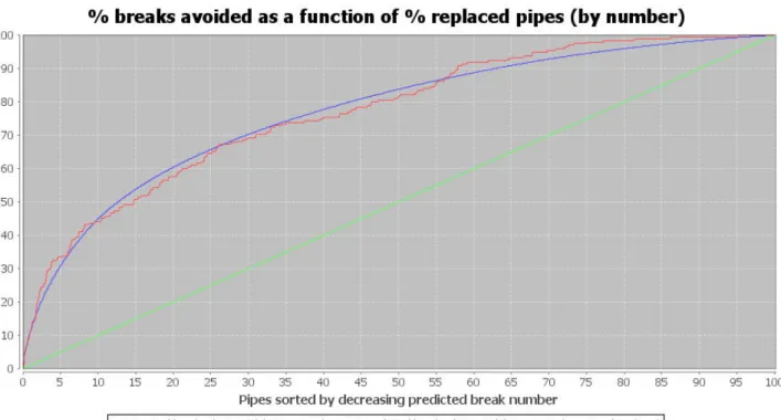
After having sorted the pipes by descending number of predicted breaks per year, the proportion of the number of actual breaks during the validation period can be expressed as a function of the number of pipes represented by the red curve in Figure 1 – X-axis represents percentage of number of pipes. A random ranking of pipes corresponds closely to that described by the function y = x (green curve). Two indicators are defined:
• An: Area under the red curve.
• C5n: Percentage of actual breaks during the validation period on 5% of the number of pipes sorted by descending number of predicted breaks.
For a random ranking, An is close to 0.5 and C5n is closed to 5%. The prediction is therefore more satisfactory when An and C5n are greater. In all cases, An and C5n are less than 1 (100%).
If a significant proportion of long pipes make up the pipes most at risk then this might lead to an optimistic vision of the model quality. 5 % of the number of pipes could, for example, represent 15% of the network length. For this reason an alternative ranking method is proposed in complement: After having sorted the pipes by descending predicted break rate, the proportion of the number of actual breaks during the validation period can be expressed as a function of the relative cumulative length of pipes. Using the same method as above, similar indicators can be calculated: Al and C5l
The validation allows the user to choose a model with satisfactory predictive performances. He can then calculate break predictions over any period.
USING THE RESULTS OF THE “CASSES” FREEWARE
The main results from the software are the predicted number of breaks and break rate for each pipe.
Comparing break evolution with different rehabilitation strategies
The first use of break prediction results is creating a hierarchy of at-risk pipes, sorting the pipes either according to decreasing predicted number of breaks or according to decreasing predicted break rate. While using number of breaks tend to select preferentially long pipes, using break rate tend to select preferentially short pipes (Poulton et al 2007).
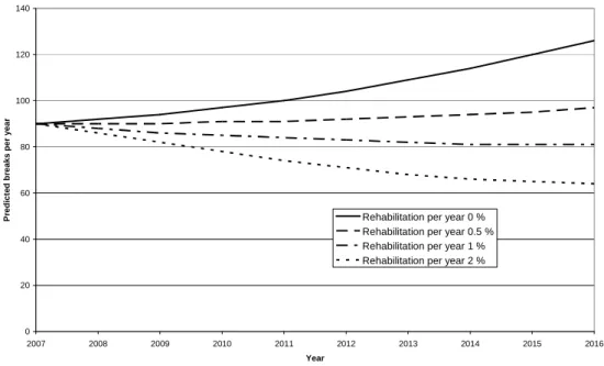
Several tests carried out by Cemagref, notably with data from Oslo water network (Norway) demonstrate that the LEYP model provides a good estimation of the number of breaks predicted. So, it is possible to calculate year-by-year, a forecast of the overall number of breaks in a network. The same calculations can be done applying different rehabilitation policies based on a hierarchy of at-risk pipes built with the model. This allows the evolution of the number of breaks to be compared for different rehabilitation policies.
SAUR FRANCE (a French water company), uses freeware “Casses” in this way. Figure 2 represents the case of a French rural drinking network 550 km long. The significant covariates of the model are diameter, length, material and pressure. If no rehabilitation is carried out, the number of breaks will increase from 90 in 2007 to 126 in 2016. If a rehabilitation rate of 0.5% per year is used, the number of break will almost stabilise. For any greater rehabilitation rates, the break rate will fall.
0 20 40 60 80 100 120 140 2007 2008 2009 2010 2011 2012 2013 2014 2015 2016 Year P re d ic te d b re a k s p e r y e a r
Rehabilitation per year 0 % Rehabilitation per year 0.5 % Rehabilitation per year 1 % Rehabilitation per year 2 %
Figure 2: Break evolution with different rehabilitation strategies
Feeding multicriteria decision tools
Many tools dedicated to prioritise pipes for rehabilitation use a mulicriteria approach. Examples include Care-W integrated decision support system (Le Gauffre et al 2005) and SIROCO, a decision support system for rehabilitation adapted for small and medium size water distribution companies developed by “G2C Environnement” and Cemagref (Renaud et al 2007). The multicriteria tools use indicators which, usually, include the rate of pipe breaks.
The freeware “Casses” can work as a “slave” of an integrated application. This is the case within the SIROCO software. In order to overcome the problem of critically small databases, the SIROCO approach involved creating a database that amalgamates data from several companies. It is based on a geographic information system (GIS) which enables a structured data organisation. Same data can be used as potential covariates in the LEYP model and as multicriteria analysis indicators. Four of the seven criteria need the predicted break rate value for their calculation:
• Linear index of hydraulic criticality. The impact of the pipe in terms of continuity of water supply to users is calculated using hydraulic modelling combined with break prediction (Bremond and Bertin 2001). It is here worth pointing out that the relevance of the hydraulic criticality index could be substantially improved by using a pressure dependent model for hydraulic computations.
• Road traffic disturbance index. This combines the level of road traffic above the pipe and its break rate.
• Repair/Replacement cost ratio. This compares the annual cost of repairs of the pipe knowing the predicted number of breaks and the annual depreciation allowance of the pipe.
• Index of local disturbance to continuity of service. This combines the annual time of unavailability of the pipe (deduced of the predict number of breaks) and the vulnerability of the users directly connected to the pipe.
The user can automatically produce the input data files and then, use the “Casses” freeware to calibrate a model and calculate break predictions. After that, he can use selected results to run the SIROCO analysis and rank pipes as rehabilitation candidates.
CONCLUSION
With the ageing of the network, drinking water utilities have to plan the rehabilitation of their pipes. Many of them now have large databases with detailed description of the pipes and break history of each pipe. Besides that, the last twenty years has seen significant research concerning statistical tools dedicated to forecast pipe breaks and provide relevant models.
A new step is to design tools using these models and that are available to be used by the technical staffs of water utilities or by consultants. To make that possible, it is necessary to be able to cope with the wide diversity of data and to design tools dedicated to prepare data for the calculations. Furthermore, the user must be assisted to calibrate a relevant model. Then, the results of break predictions can be used to compare rehabilitation strategies and to rank pipes as rehabilitation candidates using multicriteria approaches.
After having developed the break prediction freeware “Casses”, based on the LEYP model and having integrated it in the decision support software SIROCO, Cemagref continues working in the field to improve the model and the tools:
• Research is ongoing to integrate “time dependant” covariates like climate in the LEYP model (Babykina et al 2009)
• The use of break prediction models to assess the service life distribution of pipes is also under study.
References
Andersen, P.K., Borgan, O., Gill, R., Keiding, N., (1993).Statistical Models Based on Counting Pracesses, 1st Edition. Springer-Verlag, New York.
Babykina, G., Couallier, V., Le Gat,Y. (2009). Modeling failures of repairable systems under "worse than old" assumption. 6th International Conference on "Mathematical Methods in Reliability. Theory. Methods. Applications.". Moscou.
Bremond B.,Bertin S. (2001) : Reliability of a drinking water supply system. IWA Brno
Cemagref (2008), « Casses » User Manual. available at https://casses.cemagref.fr/ (accessed 15 september 2009)
Eisenbeis, P. (1994), Modélisation statistique de la prévision des défaillances sur les conduits d'eau potable (Statistical modeling of drinking water pipes break prediction) . PhD thesis, Université Louis Pasteur Strasbourg, 1994.
Eisenbeis, P., Laffrechine, K., Rostum, J., and Tuhovcak, L. (2005). Réhabilitation des réseaux d'eau potable : Des logiciels pour le calcul d'indicateurs techniques (Drinking water networks rehabilitation : Tools for technical indicators calculations) TSM, 2005 - 1, 90 - 97.
Lawless, J.F., (1987). Regression methods for poisson process data. Journal of the Americain Statistical Association, Theory and Methods 82 (399), 808-815.
Le Gat, Y and Eisenbeis P. (2000), Using maintenance records to forecast failures in water networks, Urban Warter, 2:173-181,
Le Gat, Y. (2002). Evaluation de la performance d’un modèle de prévision de casses en réseau d’adduction d’eau potable (Performance evaluation of a break prediction modele for drinking water networks) Mémoire de DEA, Université de Bordeaux 2.
Le Gat Y (2009), Etude du Processus de Yule Non Homogène – Application à la modélisation du risque de casses en réseau d’AEP (Study of the non homogeneous Yule process – Application to drinking water pipes failure risk modelling), PhD thesis, ENGREF Paris, (in preparation).
Le Gauffre, P., Laffrechine, K., Bauer, R., Poinard, D., and Schiatti, M. (2005). Réhabilitation des réseaux d'eau potable : Des outils multicritères pour la programmation annuelle (Drinking water networks rehabilitation: Multicriteria tools for annual programming . TSM, 2005 - 1, 81 - 89.
Poulton, M., Le Gat, Y. Bremond, B. (2007), The impact of pipe segment length on break predictions in water distribution systems, IWA Lesam 2007 conference proceedings
Renaud, E., De Massiac, J.C., Bremond, B., Laplaud, C. (2007). SIROCO, a decision support system for rehabilitation adapted for small and medium size water distribution companies, IWA Lesam 2007 conference proceedings
Ross, S., (1983). Stochastic processes. John Wiley and Sons, New York.
Torterotot, J., Werey, C., Rebelo, M., and Cravero, J. (2005). Réhabilitation des réseaux d'eau potable : Les processus de décision et le projet CARE-W (Drinking water networks rehabilitation : Decision processes and Care-W project) . TSM, 2005 - 1, 56 - 64.