Global observations of the zonal drift speed of equatorial ionospheric plasma bubbles

(1)

HAL Id: hal-00317621

https://hal.archives-ouvertes.fr/hal-00317621

Submitted on 23 Sep 2004

HAL is a multi-disciplinary open access

archive for the deposit and dissemination of

sci-entific research documents, whether they are

pub-lished or not. The documents may come from

teaching and research institutions in France or

abroad, or from public or private research centers.

L’archive ouverte pluridisciplinaire HAL, est

destinée au dépôt et à la diffusion de documents

scientifiques de niveau recherche, publiés ou non,

émanant des établissements d’enseignement et de

recherche français ou étrangers, des laboratoires

publics ou privés.

Global observations of the zonal drift speed of equatorial

ionospheric plasma bubbles

T. J. Immel, H. U. Frey, S. B. Mende, E. Sagawa

To cite this version:

T. J. Immel, H. U. Frey, S. B. Mende, E. Sagawa. Global observations of the zonal drift speed of

equatorial ionospheric plasma bubbles. Annales Geophysicae, European Geosciences Union, 2004, 22

(9), pp.3099-3107. �hal-00317621�

(2)

SRef-ID: 1432-0576/ag/2004-22-3099 © European Geosciences Union 2004

Annales

Geophysicae

Global observations of the zonal drift speed of equatorial

ionospheric plasma bubbles

T. J. Immel1, H. U. Frey1, S. B. Mende1, and E. Sagawa2

1_{Space Sciences Laboratory, University of California Berkeley, USA} 2_{Communications Research Laboratory, Tokyo, Japan}

Received: 3 October 2003 – Revised: 31 January 2004 – Accepted: 9 February 2004 – Published: 23 September 2004 Part of Special Issue “Equatorial and low latitude aeronomy”

Abstract. Space-based measurements from an imager

aboard the high-apogee NASA-IMAGE satellite allows for global-scale observations of nightside ionospheric densities and structure. Such a view cannot be provided by imagers in near-Earth orbit or based on the ground. The IMAGE Spec-troscopic Imager (SI) isolates the Far-ultraviolet (FUV) O I 135.6 nm emission which is produced through radiative re-combination of O+. These observations clearly show the dis-tribution of FUV emissions of the equatorial airglow bands over the range of local times between the evening terminator to points well after midnight. Determination of plasma drift speeds in these local time sectors is performed by identifica-tion and subsequent tracking of localized depressions in the FUV emissions. This determination is made for nearly 200 plasma bubbles in the March-May period of 2002. Important findings of this study include (1) an unambiguous association between Dst and zonal plasma drift speeds, and (2) a

longi-tudinal dependence of the zonal plasma drift speeds, with a peak around the Indian sector. The first effect is attributed to penetrating ring current electric fields, while the second is apparently due to a longitudinal variability in the vertical po-larization electric fields that directly affects the zonal plasma drift speeds.

Key words. Ionosphere (Equatorial ionosphere, Electric

fields and currents, Ionosphere-magnetosphere interactions, Ionospheric irregularities)

1 Introduction

Recent studies of the nightside equatorial ionosphere demon-strate the utility of global-scale far-ultraviolet (FUV) imag-ing for retrievimag-ing important ionospheric parameters. Usimag-ing global-scale images of the far-ultraviolet emissions produced by recombination of ionospheric O+, Immel et al. (2003) and Sagawa et al. (2003) found that plasma drift speeds

Correspondence to: T. J. Immel

([email protected])

in the ionospheric anomalies could be determined through analysis of multiple successive images of the equatorial air-glow bands. Such a determination depends on the presence of embedded brightness irregularities, a requirement eas-ily fulfilled by the presence of equatorial ionospheric bub-bles. Once produced in the post-sunset equatorial iono-sphere, plasma bubbles appear as localized decreases in air-glow brightness and can be tracked across the nightside to determine their zonal drift speed. Under the assumption that these depletions are embedded in the surrounding plasma, one can equate the bubble drift speed with the drift of the am-bient ionospheric plasma (Mendillo and Baumgardner, 1982; Taylor et al., 1997; Pimenta et al., 2003).

In the above noted study, Immel et al. (2003) determined the globally averaged speed of zonal plasma drifts from IMAGE/FUV images of the O I 135.6 nm emission during March-May 2002. These were compared to zonal drifts de-termined by the Jicamarca radar from data obtained over sev-eral years (Fejer et al., 1991), whereupon it was determined that the global-averaged zonal drifts in the equatorial iono-spheric anomaly were generally higher than those measured at the magnetic equator, especially at early local times. This latitudinal shear effect was noted earlier by Aggson et al. (1987), using in-situ plasma drift observations by the polar-orbiting DE-2 satellite. Recent studies confirm and help to explain this observation (Martinis et al., 2003), as F-region drifts have a stronger initial effect on plasma flux tubes that terminate in the anomalies than on plasma in flux tubes that terminate closer to the equator (with lower apex altitudes).

The current study is an extended investigation of the plasma drifts observed in the aforementioned year 2002 pe-riod. Of particular interest is the global distribution of plasma drift speeds, and the factors that may influence or cause sys-tematic localized or global variability in these drift speeds. The significant variations in magnetic field strength, declina-tion, and geographic latitude along the magnetic equator are factors that may well have (heretofore unobserved) localized effects on plasma drift speeds and the ionosphere in general.

(3)

3100 T. J. Immel et al.: Global observations of equatorial ionospheric plasma drift speeds The zonal drift of equatorial ionospheric F-region plasma

was first described by Woodman (1972), using measurements from the radar facility at Jicamarca, Peru. Since then, nu-merous studies of the dependence of the zonal plasma drift on neutral wind interactions, solar irradiance, and geomag-netic activity have been undertaken (e.g. Fejer et al., 1981, 1985, 1991; Fejer, 1993; Fejer and Scherliess, 1998; Sobral and Abdu, 1991; Sobral et al., 1999; Scherliess and Fejer, 1998; Valladares et al., 1996; de Paula et al., 2002). The work described in this report is the first space-based imaging study that addresses the topics previously studied using only ground-based or in-situ measurements.

Several studies have investigated the properties of the equatorial ionosphere with specific attention to longitudi-nal variations in the properties of the plasma. The global distribution of vertical plasma drifts was examined by Fe-jer et al. (1995), using data from the AE-E satellite. How-ever, AE-E only measured cross track drifts, and given its low-inclination orbit (∼19◦), the zonal speeds were gener-ally along the satellite track and not unambiguously separa-ble from the satellite velocity. Coley et al. (1994) did look at the global distribution of low-latitude zonal plasma drifts from the polar-orbiting DE-2 satellite, but as a function of local time rather than longitude. In an earlier study of DE-2 data, Coley and Heelis (1989) state that aside from a some-what different strength and location of the evening zonal drift reversal, the zonal drifts do not depend on longitude. Maynard et al. (1995) performed a thorough analysis of low-latitude drift velocities measured by the San Marco D satel-lite, showing the variability as a function of solar radio flux, lunar phase, season, and longitude. While the zonal plasma drifts showed little variation with longitude, it was found that the vertical drifts had a significant longitudinal dependence, with a maximum dayside vertical drift speed in the Indian sector. The San Marco D satellite had the lowest inclination of all the satellites discussed here (∼3◦).

This research aims to provide a new and comprehensive set of observations of low-latitude plasma drift speeds over several months of time between equinox and solstice. In particular, the goal is to determine the degree of influence of factors such as magnetic activity, solar output, or ge-ographic location. The IMAGE/FUV data set provides a unique global view with simultaneous measurements over >90◦_{of longitude, and continuous, extended (>5 h)}

observa-tions of changes in densities in the low-latitude ionospheric anomalies, including individual plasma bubbles. Its utility in making ionospheric observations should prove to benefit the understanding of the physical processes influencing the low-latitude ionosphere.

2 Instrumentation: IMAGE/FUV SI-13

The NASA-IMAGE satellite was placed into a highly ellip-tical polar orbit by a Boeing Delta II launch vehicle on 25 March 2000. Apogee was originally at 40◦north latitude, but through apsidal motion the apogee reached 90◦N in 2001,

and by March 2002 was again approaching 40◦_{N latitude,}

with right ascension of apogee 180◦_{away from the initial}

or-bit. The low latitude of apogee in 2002 provided observation times well suited for equatorial measurements. The orbital geometry was equally favorable at the beginning of the mis-sion, but the imager was operated primarily as a high-latitude auroral imager at that time. The focus of this study remains, therefore, on the 2002 observations.

The Spectrographic Imager (SI) on board IMAGE has two FUV wavelength channels, one to obtain images of Doppler-shifted hydrogen emissions at 121.8 nm, originating in the proton aurora, and another to spectrally separate and ob-tain images of the 135.6 nm emission of O I (Mende et al., 2000). In the terrestrial environment, this emission of O I generally has two causes; either excitation by impact of ener-getic electrons produced by solar Extreme-ultraviolet (EUV) photoionization or ionization through precipitation of auro-ral particles, or by radiative recombination of ionospheric O+. The later reaction is also responsible for the 630.0 and 777.4 nm emissions often observed by ground-based ob-servers at equatorial or mid-latitude stations (Weber et al., 1978; Meriwether et al., 1985; Makela et al., 2001).

The 135.6 nm channel of the SI is usually called SI-13. The SI-13 is insensitive to the bright, optically thick emis-sions of O I at 130.4 nm, though with its 5-nm passband centered at 135.6 nm it is sensitive to a particular N2Lyman

Birge Hopfield (LBH) band emission at 135.4 nm. For ob-servations of the aurora or the daytime airglow this must be taken into consideration. However, in the nighttime middle-to-low latitude ionosphere, the LBH emission is basically ab-sent, and the signal in the SI-13 is purely due to the 135.6 nm emissions. Final stellar calibrations (Frey et al., 2003) report an instrumental sensitivity of 15.3 counts per 1000 Rayleighs (R) per pixel (5-s exposure) of O I 135.6 nm emissions. The counting rates for observations in the equatorial ionospheric anomaly regions generally peak around 5–8 counts per pixel, indicating emissions less than 500 R, close to the expected brightness.

With a 14.2-h orbit period, the imager can dwell on low-latitude emissions for 6–8 h per orbit. As shown by Immel et al. (2003), the duration of the observation is sufficient to observe any significant changes in the brightness and/or morphology of the emissions originating in the ionospheric anomaly. Though the images are global in scale, the lati-tude of apogee in the March-May 2002 time of interest is not ideal for observations of the southern anomaly, or even of the northern anomaly in regions where the magnetic equator dips well into the Southern Hemisphere (i.e. South America). The combination of this fact and a known seasonal reduction in the occurrence of spread-F and ionospheric bubbles in the South American sector beginning in April-May (Valladares et al., 1996) result in a total lack of bubble observations over 70◦of longitude in the South American sector for the 2002 observational season.

(4)

-30 -30 -30 -20 -20 -20 -20 -10 -10 -10 -10 10 10 10 10 10 20 20 20 20 20 30 30 30 30 30 0 0 0 0 0 -30 -30 -30 -20 -20 -20 -20 -10 -10 -10 -10 10 10 10 10 10 20 20 20 20 20 30 30 30 30 30 0 0 0 0 0 May 1, 2002 (Day 121), 09:00 UT IMAGE/FUV SI-13 135.6 OI emissions 14 minute integration SSL, UC Berkeley 0.0 0.0 0.1 0.1 0.2 0.2 0.3 0.3 ≥0.4 ≥0.4 Brightness(kRayleigh) Brightness(kRayleigh) IMAGE/FUV SI-13 135.6 OI emissions 14 minute integration SSL, UC Berkeley May 3, 2002 (Day 123), 14:28 UT

(a)

(c)

(b)

(d)

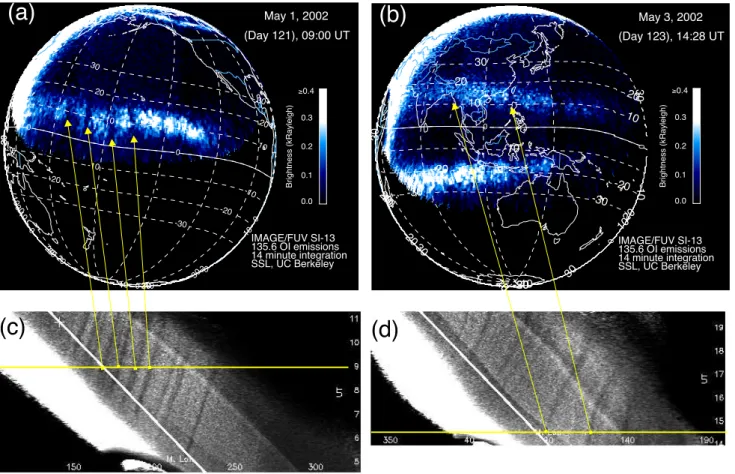
Fig. 1. Two 135.6 nm imaging examples with keograms of integrated brightness. Figures 1a, b show images resulting from integrations of seven 5-second SI-13 exposures obtained during 14 min of nominal imager operations with 2-min imaging cadence. These are mapped onto a projection of geographic coordinates centered at 22:00 LT on days 121 and 123 of 2002, respectively. Figures 1c, d show keograms of the latitudinally integrated brightness in the northern airglow band for a period of observations including the images shown above. The horizontal scale of the keograms indicates magnetic longitude, where 0◦longitude coincides with Greenwich, and the vertical scale indicates UT. The time of the image is indicated with a horizontal yellow line and the features in the images associated with depletions in the keogram are noted with arrows.

3 Data analysis

3.1 Determination of drift speeds, two examples

Figure 1 shows a pair of images from early May 2002, mapped to an orthographic projection of geographic coor-dinates with contours of magnetic latitude and longitude su-perposed. The center of the projection is at the geographic equator and 22:00 LT. The upper left image is the average brightness observed in 7 successive images (obtained over 14 min) from the SI-13 instrument, beginning at 09:00 UT on 1 May. The upper right image is a similar projection of the average of 7 successive images obtained after 14:28 UT on 3 May. Each of these images shows the emissions from the northern equatorial airglow band, that extend from the re-gion of bright airglow at the western edge of the disc across the nightside. The 3 May image also shows the southern air-glow band, whose brightness is enhanced due to the effect of limb brightening, as the southern band was near the imaging horizon at this time.

Each of these images is obtained at a time during which several low-latitude ionospheric plasma bubbles are gener-ated and proceed to drift across the nightside. Below each image is a record of the latitudinally-integrated brightness of the northern airglow band as a function of magnetic longi-tude and UT. Every image is processed and represented as a single row of pixels in this keogram. A horizontal yellow line underlies the row of pixels corresponding to the above image. The vertical scales are identical so the vertical size of the keogram is representative of the total time of obser-vation. In each keogram, airglow depletions associated with plasma bubbles appear as dark stripes, depressions in bright-ness which drift eastward with time. The depletions can also be seen in the images, and the locations of the bubbles in the images are identified by arrows originating at their cor-responding location in the keograms. The white line in the keograms indicates the motion of the location of 20 h Mag-netic Local Time (MLT) in the keogram.

The 1 May case shows several well-defined, localized de-pletions in airglow brightness. Four plasma bubbles are

(5)

3102 T. J. Immel et al.: Global observations of equatorial ionospheric plasma drift speeds 40 60 80 100 120 Magnetic Longitude 14 15 16 17 18 19 UT(hours) 40 60 80 100 120 Magnetic Longitude 0 2 4 6 8 10 12 14 Driftspeed(deg/hour) 160 180 200 220 240 Magnetic Longitude 5 6 7 8 9 10 11 UT(hours) 160 180 200 220 240 Magnetic Longitude 0 2 4 6 8 10 12 14 Driftspeed(deg/hour) (a) (c) (b) Day 121 Day 123 (d)

Fig. 2. Locations and velocities of major brightness depletions from keograms of Fig. 1. (a) The locations of 5 brightness decreases seen in the keogram of Fig. 1c are determined and plotted as a function of MLon vs. UT. (b) The drift speed of each depletion shown in 2a is shown as a function of MLon. (c, d) These panels repeat the presentation of 2a, b, but following three brightness depletions from Fig. 1d.

clearly identifiable in the image and in the keogram. The 3 May case does not have such strong depletions, but the lo-cations of two depletions can still be identified in both the keogram and the image. A comparison of these keograms reveals that the 1 May depletions show a much more steady drift across the nightside than the 3 May case, when the drifts are more variable and often more rapid.

Figure 2 shows the locations and speeds of the most eas-ily identifiable bubbles. Figures 2a and 2b show the bubbles’ positions and drift speeds, respectively, in Magnetic Longi-tude (MLon) vs. UT coordinates for the 1 May period of interest. The positions (longitudes) are determined for each row of the keogram from a Gaussian function least-squares fitted to the brightness vs. ML on data around the position of the bubble. The initial position is determined by hand, then determined by a Gaussian fitting of a 13-point subset of the row of counts centered on the last observed position of the depletion for all subsequent points. If the fitting procedure fails to converge to a solution, the position of the minimum counting rate is used. The speeds are determined using a 4th degree polynomial, least-squares fitted to the position of each plasma bubble vs. UT (as shown in Fig. 2a). The derivative of this fit, i.e. the fitted speed of the plasma bubble, v, is de-termined. These plots show that the 1 May period exhibited several bubbles between geomagnetic longitudes 160◦ and 240◦, drifting at speeds of around 5◦/hour, on average. The low rate of change in drift speeds seen in the 1 May keogram (Fig. 1c) is reflected here in the velocity plot.

The 3 May locations and velocities are shown in Figs. 2c and 2d, respectively, showing finally the velocities of three plasma bubbles observed between 50◦and 130◦MLon. The

westernmost bubble displays variability similar to that seen on 1 May, with a peak speed of 10◦_{/hour around 50 MLon,}

with gradually slowing speeds afterwards. The next bubble to the east shows a general increase in velocity from 3◦ to 9◦/hour between 85◦ and 102◦MLon, followed by a slow-down back to ∼6 m/sec around 115◦. The easternmost bub-ble shows only a consistent increase in velocity between 115◦ and 138◦MLon.

These later bubble drifts conflict with the generally ob-served variation, that nightside plasma drift speeds slow with local time (Fejer et al., 1991). The reason for this variation and the significant difference between the day 123 and 121 plasma drifts is not clear from the images, as in each case the airglow bands are nominally located around ± 10–15◦ magnetic latitude, and the level of magnetic activity is about the same on the two days (average Kp121(Dst121)= 1.3 (5 nT)

vs Kp123(Dst123)= .9 (1.3 nT)). The most obvious difference

between the two observations is that the drifts are being mea-sured over different parts of the Earth, separated by 100◦of longitude. Whether the drift speed behavior observed on day 123 is unique to this imaging time/geographic sector or is ob-served more frequently will be investigated in the course of this study.

3.2 Relation of drift speeds to magnetic and solar activity 3.2.1 Kpand Dstdependences

Before analyzing the data for any global variations in drift speed, other influencing factors must be determined, and if necessary, removed from the data set or otherwise accounted for. One area of interest is the effect of magnetic activity on low-latitude electric fields, that will in turn affect the plasma drift speeds observed.

There are a total of 104 plasma depletions observed dur-ing the days between 87–129, 2002 that are tracked to deter-mine drift speeds. The level of magnetic activity during these times is such that most bubbles are seen to occur during pe-riods of low-to-moderate activity, where Kp≤3+. Several

bubbles were seen around the time of the 17–21 April storm period, where Kpwas in the range of 4–6. These are the only

observations at high levels of activity, however, which may be too few for a good statistical analysis of the effects of high magnetic activity.

To determine any possible effect of geomagnetic activity on plasma drift speeds, the drift velocities are determined for all bubbles as described in the previous section. The MLT of the bubble and the magnetic planetary K index (Kp) at each

imaging time is recorded along with the velocity, and the av-erage velocity is determined in one hour bins of MLT, and in bins of Kp, where, for example, Kp=3−, 3oand 3+ are

considered equivalent. The average drift speed as a function of Kp can therefore be plotted in separate bins of MLT, as

shown for six MLT bins in Fig. 3. In these panels, heavy diamonds indicate values for which the standard deviation of the mean velocity (σm) is <50% of the actual value. The

(6)

0 2 4 6 8 Kp 0 2 4 6 8 10

Drift Speed (deg/hr)

MLT=19-20 Hrs. 0 2 4 6 8 Kp 0 2 4 6 8 10

MLT=20-21 Hrs. 0 2 4 6 8 Kp 0 2 4 6 8 10

MLT=21-22 Hrs. 0 2 4 6 8 Kp 0 2 4 6 8 10

MLT=22-23 Hrs. 0 2 4 6 8 Kp 0 2 4 6 8 10

MLT=23-24 Hrs. 0 2 4 6 8 Kp 0 2 4 6 8 10

MLT=0-1 Hrs.

Fig. 3. Kpdependence of the drift speeds in 6 magnetic local time

sectors. In each plot, the most statistically significant points are shown with heavy diamonds and error bars. Less significant points are shown with light diamonds and no error bar. A linear least-squares fit is calculated and overlaid in each panel. The average coefficient of linear correlation over these six magnetic local time sectors is 0.63.

Light diamonds are points where σmis greater than 50% of

the speed, though these standard deviations are not shown. Each frame of Fig. 3 shows a slightly different variation in drift speeds vs. Kp, but the trend towards lower values

with increasing Kp is clear in the 20:00–23:00 MLT range.

Inclusion of the high standard deviation points would ex-tend the trend to 19:00–24:00 MLT. In each panel, a line is least-squares fitted to the points represented by the heavy di-amonds. The average of the coefficients of linear correlation is −0.63. This is a fair correlation, and shows a significant relation between drift speeds and Kp.

A similar analysis is carried out using the geomagnetic storm index, Dst, as the indicator of magnetic activity. The

average plasma drift speeds are now determined in one hour bins of MLT and 25 nT bins of Dst. The average speeds are

shown in Fig. 4, where heavy and light diamonds again de-mark points with σm less or greater than 50% of the mean

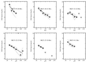
speed, respectively. This set of figures shows a very defi-nite decrease in drift speed with decreasing Dst (increasing

magnetic storm activity) across all local time sectors. Linear lines are fitted to the heavy diamonds (in a manner similar to that used for Fig. 3), and the average coefficient of linear correlation in the 06:00 MLT sectors is −0.93. This indicates an excellent correlation between the storm time ring current strength and the low-latitude zonal plasma drift speeds.

The result of this analysis is that any study of the longitu-dinal variation in drift speed must take into account the value of the Dst index, and either sort the data by that index or

determine a correction factor to apply based on the value of Dst. The relation with Kp is noteable, but of lesser

impor-tance than Dst, and probably not causative. The linear fits

shown in the Dst plots characterize the variation of the drift

speed, and are used to develop correction factors that may be

50 0 -50 -100 -150 Dst 0 2 4 6 8 10

MLT=19-20 Hrs. 50 0 -50 -100 -150 Dst 0 2 4 6 8 10

MLT=20-21 Hrs. 50 0 -50 -100 -150 Dst 0 2 4 6 8 10

MLT=21-22 Hrs. 50 0 -50 -100 -150 Dst 0 2 4 6 8 10

MLT=22-23 Hrs. 50 0 -50 -100 -150 Dst 0 2 4 6 8 10

MLT=23-24 Hrs. 50 0 -50 -100 -150 Dst 0 2 4 6 8 10

MLT=0-1 Hrs.

Fig. 4. Dst dependence of the drift speeds in 6 magnetic local time

sectors. As in Fig. 3, the most statistically significant points are shown with heavy diamonds and error bars. Less significant points are shown with light diamonds and no error bar. A linear least-squares fit is calculated and overlaid in each panel. The average coefficient of linear correlation over these six magnetic local time sectors is 0.93.

applied to any set of drift speed observations, to normalize the observed speeds to Dst=0 nT. From this point onward, all

analyses are performed using drift speeds that are normalized to Dst=0 nT.

3.2.2 Solar 10.7 cm and EUV flux dependences

If the drift speeds measured by the FUV instrument are truly plasma drift speeds, a manifestation of the known relation between solar irradiance, zonal neutral winds and ion drifts should be revealed in an analysis of these data (Biondi et al., 1991, 1999; Fejer et al., 1991). Until the late 1980s, no con-sistent direct measure of solar EUV irradiance was available, but a good long-term correlation between the EUV flux and the 10.7 cm solar radio flux provided a ground-based and consistently measurable proxy for solar EUV. Consistent, di-rect measurements are now available, however, and the EUV fluxes in narrow (26–34 nm) and wide (1–50 nm) passbands have been provided by the SOHO-SEM instrument since the beginning of the NASA-IMAGE observations (Judge et al., 1998). Here, comparisons between each of these parameters and the measured plasma drift speeds are made in one hour bins of MLT, similar to the analyses of Section 3.2.1. As noted before, all of these data are normalized to Dst=0 nT in

the manner described in Sect. 3.2.1.

To compare the plasma drift speeds and F10.7, the average

drift speeds are determined in 1 h bins of MLT and 25 Jan-sky (Jy) bins of solar radio flux. The results are shown for 6 bins of MLT in Fig. 5. Heavy (light) diamonds indicate val-ues where σmwas less (greater) than 50% of the mean, and v±σmis indicated by dashed lines. In each panel, a linear fit

to the data, weighted by the inverse of σm, is overlaid. In

(7)

3104 T. J. Immel et al.: Global observations of equatorial ionospheric plasma drift speeds 100 120 140 160 180 200 220 240 F107 0 2 4 6 8 10

MLT=19-20 Hrs. 100 120 140 160 180 200 220 240 F107 0 2 4 6 8 10

MLT=20-21 Hrs. 100 120 140 160 180 200 220 240 F107 0 2 4 6 8 10

MLT=21-22 Hrs. 100 120 140 160 180 200 220 240 F107 0 2 4 6 8 10

MLT=22-23 Hrs. 100 120 140 160 180 200 220 240 F107 0 2 4 6 8 10

MLT=23-24 Hrs. 100 120 140 160 180 200 220 240 F107 0 2 4 6 8 10

MLT=0-1 Hrs.

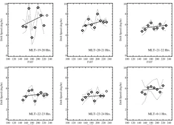
Fig. 5. F10.7dependence of the drift speeds in 6 magnetic local time

sectors. As in Fig. 3, the most statistically significant points are shown with heavy diamonds and error bars. Less significant points are shown with light diamonds and no error bar. A linear least-squares fit is calculated and overlaid in each panel. The average coefficient of linear correlation over these six magnetic local time sectors is 0.34.

increase in drift speed with solar activity. The correlation of linear correlation is determined for each panel, the average of the 6 panels is 0.34. Though the correlation is not great, it indicates a moderate degree of confidence in the trend toward positive slopes suggested by each of the 6 separate fits.

Comparisons of the drift speed with solar EUV flux is done in a very similar manner as the previous analysis of the F10.7

dependence. In this case, the data are binned in units of 109 photons/cm2/sec, and in this case only the wide-band data are used. The range of solar fluxes over the period of interest is from 52–64 ×109photons/cm2sec. Unlike the F10.7

mea-surement, the space-based detector is overwhelmed by ener-getic solar proton fluxes occurring during and after flares, so the days between 17–23 April 2002 are not included. The re-sults of this analysis are shown for six MLT sectors in Fig. 6. The overall increase in the zonal drift speed with increas-ing solar EUV flux is clear in each sector of MLT. Lin-ear least-squares fits to the points represented by heavy di-amonds all have a positive slope. The average coefficient of linear correlation is 0.56, which is not outstanding, but is more significant than the coefficient calculated in the above-performed F10.7analysis. This is expected, as the EUV flux

directly affects thermospheric temperatures, pressure gradi-ents, and in the end, zonal neutral winds and vertical electric fields. The F10.7is just a proxy for this, with a better

correla-tion over longer terms than over periods of significant daily variation (as noted by Hedin (1984)), such as is the case in March–May 2003.

3.3 Longitudinal Drift Speed Variability

To this point, the approach has been to determine the influ-ence of geophysically important effects through comparisons

50 55 60 65 70 SEM Wide/109 0 2 4 6 8 10

MLT=19-20 Hrs. 50 55 60 65 70 SEM Wide/109 0 2 4 6 8 10

MLT=20-21 Hrs. 50 55 60 65 70 SEM Wide/109 0 2 4 6 8 10

MLT=21-22 Hrs. 50 55 60 65 70 SEM Wide/109 0 2 4 6 8 10

MLT=22-23 Hrs. 50 55 60 65 70 SEM Wide/109 0 2 4 6 8 10

MLT=23-24 Hrs. 50 55 60 65 70 SEM Wide/109 0 2 4 6 8 10

MLT=0-1 Hrs.

Fig. 6. Solar EUV flux dependence of the drift speeds in 6 magnetic local time sectors. As in Fig. 3, the most statistically significant points are shown with heavy diamonds and error bars. Less signifi-cant points are shown with light diamonds and no error bar. A linear least-squares fit is calculated and overlaid in each panel. The aver-age coefficient of linear correlation over these six magnetic local time sectors is 0.56.

with magnetic and solar indices or measurements. The ve-locity measurements have been averaged in bins of these fac-tors and MLT, with no regard to the terrestrial location of the measurement. In this section, the importance of terres-trial location is investigated. Using the results of the earlier sections, it is possible to remove geophysically controlled variability to better reveal geographic dependences. Though all of the comparisons yielded results of some significance, the DstMLT analysis showed very significant linear

correla-tions, from which correction factors for subsequent removal of the Dst effect are determined. Corrections for Dst effects

have already been applied in Sect. 3.2.2, and are applied in this section as well.

The Dst-corrected plasma drift velocities are shown

ver-sus geomagnetic longitude in Fig. 7. In this case, as with the plots shown in Figs. 1 and 2, the 0◦_{reference is a magnetic}

meridian through Greenwich. These velocities come from 4 separate one-hour bins of MLT, from 20:00 to 24:00 MLT, proceeding from the top to bottom panel. Each diamond represents the average speed of all bubbles observed in one-degree bins of MLon. Obvious is the gap in the South Amer-ican sector, where bubbles are not observed during the entire observational period. In addition to the unfavorable seasonal effect, the number of observations in that sector is less, with only ∼2500 images containing pixels located at those longi-tudes vs. a peak imaging frequency of nearly 6000 during the same observation period (occurring around 120◦). The sea-sonal effect is discussed at length by Valladares et al. (1996), while the later effect is due to observational geometry and the southward excursion of the magnetic equator in the South American sector.

Figure 7 shows that the drift speeds are not randomly dis-tributed about a mean value, but in each MLT sector exhibit

(8)

T. J. Immel et al.: Global observations of equatorial ionospheric plasma drift speeds 3105 a peak speed between 60 and 100◦_{. In each MLT sector, this}

peak speed represents up to a 50% excursion away from the mean value. For instance, in the 20:00–21:00 MLT sector, af-ter filaf-tering the data with a 15◦wide moving median function, the peak speed is 9.9◦/h, while the mean speed is 6.5◦/h. In that sector, this peak is located just to the west of the peak in the magnetic field strength in the anomaly (determined at 15◦ magnetic latitude using the IGRF reference field). Closer to midnight, the peaks in drift speed and magnetic field strength are nearly colocated.

4 Discussion

The first notable result of this research is the correlation be-tween the solar radio flux and the low-latitude plasma drift speed, and the improved correlation when the speeds are compared directly to solar EUV flux. The covariation of drift speeds and solar indices has been noted in several research efforts (e.g. Sobral and Abdu, 1991; Fejer et al., 1991)) and is related to the increased thermospheric temperatures and pressure gradients resulting in higher neutral winds (Biondi et al., 1991). All of the studies cited here used the solar F10.7

flux as a proxy for solar EUV, but also used data from events distributed through several years of time, taking advantage of the long-term correlation between EUV flux and F10.7. In this

study, the observations are distributed over only 2 months of very active solar activity, in which case it is better to com-pare to direct EUV measurements. This is clear from the high correlation between drift speeds and solar EUV flux, as compared to F10.7.

A more significant result is the correspondence between zonal plasma drift speeds and Dst, where the eastward

night-time drifts slow with increasing level of disturbance (negative Dst). Compared to previous studies of the effect of magnetic

activity on the low latitude ionosphere, this result is outstand-ing in several respects. Scherliess and Fejer (1997) found very good correlation between low-latitude vertical plasma drifts and the auroral electrojet index (AE), given a time de-lay on the order of several hours. This differs from our results as, (1) the AE and Dst indices measure completely separate

(though related; see Kamide et al. (1998)) ionospheric and magnetospheric current systems, respectively, and (2) IM-AGE/FUV provides zonal plasma drifts where Scherliess and Fejer (1997) analyzed the vertical plasma drifts provided by the Jicamarca radar. In this work, no analysis of the time delay between the Dst and drift speeds that results in the

greatest correlation is reported, as the coefficient of linear correlation is already greater than 0.9, which is around the peak correlation found by Scherliess and Fejer (1997).

The slowing of zonal drifts in the vicinity of the iono-spheric anomaly during heightened magnetic activity is of-ten attributed, at least in part, to the perturbations to the global thermospheric wind system generated in response to increased high-latitude Joule heating. The wind perturba-tion generates electric fields that basically act to suppress the normal quiet-time ionospheric current system, an effect of

0 60 120 180 240 300 360 0 5 10 15 MLT=20-21

Average Drift Speed (deg/hour)

20 25 30 35 40 nT/1000 0 60 120 180 240 300 360 0 5 10 15 MLT=21-22

20 25 30 35 40 nT/1000 0 60 120 180 240 300 360 0 5 10 15 MLT=22-23

20 25 30 35 40 nT/1000 0 60 120 180 240 300 360 Magnetic Longitude 0 5 10 15 MLT=23-24

20 25 30 35 40 nT/1000

Fig. 7. Zonal drift speed vs. MLon in 4 Magnetic Local Time sec-tors. From top to bottom are shown the average plasma drift speed at all observed MLons in one hour bins from 20:00–24:00 MLT. Overlaid with a dashed line on each plot is the IGRF magnetic field strength at 15◦in units of 1000 nT. The peak velocities are seen in the 60-100◦MLon sector, with the peak shifting westward with increasing MLT.

which is the reduction of vertical low-latitude electric fields along with zonal neutral wind speeds (Blanc and Richmond, 1980). In this respect, it is even more interesting that the relation between Dst and zonal drift is so significant (much

more so than the relation with Kp), as the disturbance

dy-namo is driven by high-latitude inputs, which are not mea-sured by Dst. The close correspondence between v and Dst

indicates an effect of electric fields originating in the ring current, with an influence at least as great as disturbance dy-namo effects. The correspondence between zonal drift speed and Dst does not lend direct support to either the

penetra-tion of magnetospheric convecpenetra-tion electric fields (Burke and Maynard, 2000; Fejer, 2002) or to the interplanetary electric field Kelley (1989) to low latitudes as the causative mecha-nism slowing the equatorial zonal plasma drifts. However, to the extent that enhancements in the ring current and Dst are

driven by increased convection, we cannot rule out a slow-down in zonal drifts caused by penetrating convection elec-tric fields as described by Fejer and Scherliess (1998).

The greatest storm-time penetration effects are usually manifested in vertical motion of equatorial plasma, or the imposition of a zonal electric field (Tanaka, 1986; Foster and Rich, 1998). The zonal plasma drift speed variation observed here suggests that a radial electric field, possibly originating in the enhanced ring current, is present in the equatorial

(9)

F-3106 T. J. Immel et al.: Global observations of equatorial ionospheric plasma drift speeds region. Such a source is described by Ridley and Liemohn

(2002), where, in particular, the authors note the outward radial electric fields which develop on the nightside in re-sponse to enhancements in the region 2 current system oc-curring under magnetic storm conditions. Their simulation work predicts outward radial electric fields at ∼3000 km al-titude of 2–10 mV/m during magnetic storms, with Dst

rang-ing from −50 to −200 nT. The penetration of only a small percentage of the maximum value of 10 mV/m down to the F-region of the ionosphere would be sufficient to slow the zonal drifts to the degree seen in Fig. 4. That work also at-tributes the low-latitude penetration of magnetospheric elec-tric fields to the addition of ring current polarization elecelec-tric fields to the convection electric fields, a result also described in earlier research efforts (e.g. Blanc, 1978). It may well be that the zonal drift speed vs. Dst relationship described in

Sect. 3.2.1, which is here attributed to ring current enhance-ment, describes the same reduction of low-latitude plasma drifts noted by Fejer and Scherliess (1998) during periods of enhanced magnetospheric convection.

The reason for the overall longitudinal enhancement in drift speeds in the South-Southeast Asian sector is less clear. From a simple view of the physics of the low-latitude iono-sphere where the drift speed is proportional to |E|/|B|, this result is not expected. A maximum in the magnetic field should generally result in a minimum in the E×B drift speed. These data suggest that some process is at work to cause the vertical electric fields to reach large values in this sector ex-ceeding the ∼30% heightening of the magnetic field. One cause of this could be very low Pedersen conductivities in this sector. This could be a result of a localized enhancement in the daytime equatorial fountain, an effect noted by May-nard et al. (1995). The stronger evacuation of ionospheric plasma would lead to reduced low-latitude plasma densities in the afternoon sector, which would corotate to the night-side. Another possibility is that the integrated effect of ther-mospheric neutral winds on the ionosphere leads to higher drift speeds in this sector. This would occur if in this lon-gitude sector the influence of neutral winds at F-region alti-tudes is greater influence than in the E-region relative to other locations on Earth. This requires that a larger proportion of plasma along an ionospheric flux tube lie above the E-region, which could also result from an enhanced daytime uplift of the ionosphere.

5 Conclusions

This research finds significant and consistent geophysical ef-fects in the low-latitude plasma drift speed data provided by IMAGE-FUV. The first effect is a reduction of zonal drift speeds with increasing Dst. Though not entirely unexpected,

the effect is remarkably clear in the data set and reflects the strong, regular influence of electric fields originating in an energized ring current. The drift speed is controlled by a downward, polarization electric field, which must be weak-ened or countered by an upward electric field to slow the

drifts. This could originate in asymmetric separation of charges in the energized ring current, as recently described by Ridley and Liemohn (2002).

The second interesting effect is the longitudinal varia-tion in zonal plasma drift speeds. From observavaria-tions dur-ing the two months after vernal equinox, a peak in eastward zonal plasma drift speed is found to exist between 80◦ and 120◦E longitude. This is generally near, but not always co-located with, the maximum in the low-latitude geomagnetic field. The overall heightening of the drift speeds in this sec-tor may be due to a generally lower pedersen conductance caused by stronger evacuation of ionospheric plasma during the daytime (resulting in stronger polarization electric fields at night), or a different distribution of ionospheric plasma, with greater proportion in the F-region. This could also be driven mainly by the dynamics of the dayside ionosphere in this region of maximum magnetic field strength. The impor-tance of either of these possible effects cannot be decisively determined in this first report of the localized drift enhance-ment. Further study with in-situ data from satellites such as DMSP and NOAA and the new C-NOFS mission will help to clarify the drivers of the zonal drift enhancement in the Asian sector.

Acknowledgements. IMAGE FUV analysis is supported by NASA through Southwest Research Institute subcontract number 83 820 at the University of California, Berkeley, contract NAS5-96020.

Topical Editor M. Lester thanks I. H. Sastri and another referee for their help in evaluating this paper.

References

Aggson, T. L., Maynard, N. C., Herrero, F. A., Mayr, H. G., Brace, L. H., and Liebrecht, M. C.: Geomagnetic equatorial anomaly in zonal plasma flow, J. Geophys. Res.,92, 311–315, 1987. Biondi, M. A., Meriwether, J. W., Fejer, B. G., Gonzales, S. A., and

Hallenbeck, D. C.: Equatorial thermospheric wind changes dur-ing the solar cycle measurements at Arequipa, Peru, from 1983 to 1990, J. Geophys. Res., 96, 15 917–15 930, 1991.

Biondi, M. A., Sazykin, S. Y., Fejer, B. G., Meriwether, J. W., and Fesen, C. G.: Equatorial and low latitude thermospheric winds: measured quiet time variations with season and solar flux from 1980 to 1990, J. Geophys. Res., 104, 17 091–17 106, 1999. Blanc, M.: Midlatitude convection electric fields and their relation

to ring current development, Geophys. Res. Lett., 5, 203–206, 1978.

Blanc, M. and Richmond, A. D.: The ionospheric disturbance dy-namo, J. Geophys. Res., 85, 1669–1688, 1980.

Burke, W. J. and Maynard, N. C.: Satellite observations of electric fields in the inner magnetosphere and their effects in the mid-to-low latitude ionosphere, IEEE Trans, on Plasma Sci., 28, 1903– 1911, 2000.

Coley, W. R. and Heelis, R. A.: Low-latitude zonal and vertical ion drifts seen by DE 2, J. Geophys. Res., 94, 6751–6761, 1989. Coley, W. R., Heelis, R. A., and Spencer, N. W.: Comparison of

low-latitude ion and neutral zonal drifts using DE 2 data, J. Geo-phys. Res., 99, 341–348, 1994.

(10)

de Paula, E. R., Kantor, I. J., Sobral, J. H. A., Takahashi, H., San-tana, D. C., Gobbi, D., de Medeiros, A. F., Limiro, L. A. T., Kil, H., Kintner, P. M., and Taylor, M. J.: Ionospheric irregular-ity zonal velocities over cachoeira paulista, J. Atmos. Solar-Terr. Phys., 64, 1511–1516, 2002.

Fejer, B. G.: F Region plasma drifts over Arecibo: Solar cycle, sea-sonal and magnetic activity effects, J. Geophys. Res., 98, 13 645– 13 652, 1993.

Fejer, B. G.: Low latitude storm time ionospheric electrodynamics, J. Atmos. Solar-Terr. Phys., 64, 1401–1408, 2002.

Fejer, B. G. and Scherliess, L.: Mid and low-latitude prompt pene-tration ionospheric zonal plasma drifts, Geophys. Res. Lett., 25, 3071–3074, 1998.

Fejer, B. G., Farley, D. T., Gonzales, C. A., Woodman, R. F., and Calderon, C.: F region east-west drifts at Jicamarca, J. Geophys. Res., 86, 215–218, 1981.

Fejer, B. G., Kudeki, E., and Farley, D. T.: Equatorial F-region zonal plasma drifts, J. Geophys. Res., 90, 12 249–12 255, 1985. Fejer, B. G., de Paula, E. R., Gonz´alez, S. A., and Woodman, R. F.:

Average vertical and zonal F region plasma drifts over Jicamarca, J. Geophys. Res., 96, 13 901–13 906, 1991.

Fejer, B. G., de Paula, E. R., Heelis, R. A., and Hanson, W. B.: Global equatorial ionospheric vertical plasma drifts measured by the AE-E satellite, J. Geophys. Res., 100, 5769–5776, 1995. Foster, J. C. and Rich, F. J.: Prompt midlatitude electric field

ef-fects during severe geomagnetic storms, J. Geophys. Res., 103, 26 367–26 372, 1998.

Frey, H. U., Mende, S. B., Immel, T. J., G´erard, J.-C., Hubert, B., Habraken, S., Spann, J., Gladstone, G. R., Bisikalo, D. V., and Shematovich, V. I., Summary of quantitative interpretation of IMAGE far ultraviolet auroral data, Space Sci. Rev., 109, 255– 283, 2003.

Hedin, A. E.: Correlations between thermospheric density and tem-perature, solar EUV flux, and 10.7 cm flux variations, J. Geo-phys. Res., 89, 9828–9834, 1984.

Immel, T. J., Mende, S. B., Frey, H. U., Peticolas, L. M., and Sagawa, E.: Determination of low latitude plasma drift speeds from FUV images, Geophys. Res. Lett., 30, 1945, 2003. Judge, D. L., McMullin, D. R., Ogawa, H. S., Hovestadt, D.,

Klecker, B., Hilchenbach, M., Mobius, E., Canfield, L. R., Vest, R. E., Watts, R., Tarrio, C., Kuhne, M., and Wurz, P.: First so-lar EUV irradiances obtained from SOHO by the CELIAS/SEM, Solar Physics, 177, 161–173, 1998.

Kamide, Y., Baumjohann, W., Daglis, I. A., Gonzalez, W. D., Grande, M., Joselyn, J. A., McPherron, R. L., Phillips, J. L., Reeves, E. G. D., Rostoker, G., Sharma, A. S., Singer, H. J., Tsurutani, B. T., and Vasyliunas, V. M.: Current understanding of magnetic storms: Storm-substorm relationships, J. Geophys. Res., 103, 17 705–17 728, 1998.

Kelley, M. C.: The earth’s ionosphere plasma physics and electro-dynamics, Academic Press, Inc., San Diego, 1989.

Makela, J. J., Kelley, M. C., Gonzalez, S. A., Aponte, N., and McCoy, R. P.: Ionospheric topography maps usin multiple-wavelength all-sky images, J. Geophys. Res., 106, 29 161– 29 174, 2001.

Martinis, C., Eccles, J. V., Baumgardner, J., Manzano, J., and Mendillo, M.: Latitude dependence of zonal plasma drifts ob-tained from dual-site airglow observations, J. Geophys. Res., 108, 1129, 2003.

Maynard, N. C., Aggson, T. L., Herrero, F. A., Liebrecht, M. C., and Saba, J. L.: Average equatorial zonal and vertical ion drifts determined from San Marco D electric field measurements, J. Geophys. Res., 100, 17 465–17 479, 1995.

Mende, S. B., Heetderks, H., Frey, H. U., Stock, M., Lampton, M., Geller, S. P., Abiad, R., Siegmund, O. H. W., Habraken, S., Renotte, E., Jamar, C., Rochus, P., G´erard, J.-C., Sigler, R., and Lauche, H.: Far ultraviolet imaging from the IMAGE spacecraft. 3. Spectral imaging of Lyman-α and OI 135.6 nm, Space Sci. Rev., 91, 287–318, 2000.

Mendillo, M. and Baumgardner, J.: Airglow characteristics of equa-torial plasma depletions, J. Geophys. Res., 87, 7641–7652, 1982. Meriwether, J. W., Biondi, M. A., and Anderson, D. N.: Equatorial airglow depletions induced by thermospheric winds, Geophys. Res. Lett., 12, 487–490, 1985.

Pimenta, A. A., Bittencourt, J. A., Fagundes, P. R., Sahai, Y., Buriti, R. A., Takahashi, H., and Taylor, M. J., Ionospheric plasma bub-ble zonal drifts over the tropical region: a study using OI 630nm emission all-sky images, J. Atmos. Solar-Terr. Phys., 65, 1117– 1126, 2003.

Ridley, A. J. and Liemohn, M. W.: A model-derived storm time asymmetric ring current driven electric field description, J. Geo-phys. Res., 107, SMP–2, 2002.

Sagawa, E., Maruyama, T., Immel, T. J., Frey, H. U., and Mende, S. B.: Global view of the nighttime low latitude ionosphere by the 135.6 nm OI observation with IMAGE/FUV, Geophys. Res. Lett., 30, 1534–1537, 2003.

Scherliess, L. and Fejer, B. G.: Storm time dependence of equatorial disturbance dynamo zonal electric fields, J. Geophys. Res., 102, 24 037–24 046, 1997.

Scherliess, L. and Fejer, B. G.: Satellite studies of mid- and low-latitude ionospheric disturbance zonal plasma drifts, Geophys. Res. Lett., 25, 1503–1506, 1998.

Sobral, J. and Abdu, M.: Solar activity effects on equatorial plasma bubble zonal velocity and its latitude gradient as measured by airglow scanning photometers, J. Atmos. Terr. Phys., 53, 729– 742, 1991.

Sobral, J. H. A., Abdu, M. A., Takahashi, H., Sawant, H., Zamlutti, D., and Borba, G. L.: Solar and geomagnetic activity effects on nocturnal zonal velocities of ionospheric plasma depletions, Ad-vances in Space Research, 24, 1507–1510, 1999.

Tanaka, T.: Low-latitude ionospheric disturbances: Results for 22 March, 1979, and their general characteristics, Geophys. Res. Lett., 13, 1399–1402, 1986.

Taylor, M. J., Eccles, J. V., LaBelle, J., and Sobral, J. H. A.: High resolution OI (630 nm) image measurements of F-region deple-tion drifts during the Guara campaign, Geophys. Res. Lett., 24, 1699–1702, 1997.

Valladares, C. E., Sheehan, R., Basu, S., Kuenzler, H., and Es-pinoza, J.: The multi-instrumented studies of equatorial ther-mosphere aeronomy scintillation system: Climatology of zonal drifts, J. Geophys. Res., 101, 26 839–26 850, 1996.

Weber, E. J., Buchau, J., Eather, R. H., and Mende, S. B.: North-south aligned equatorial airglow depletions, J. Geophys. Res., 83, 712–716, 1978.

Woodman, R. F.: East-west ionospheric drifts at the magnetic equa-tor, Space Res., 81, 5447–5466, 1972.