by
TERENCE JOHN WALES Bachelor of Arts
University of British Columbia (1962)
SUBMITTED IN PARTIAL FULFILLMENT OF THE REQUIREMENTS FOR THE
DEGREE OF DOCTOR OF PHILOSOPHY
at the
MASSACHUSETTS INSTITUTE OF TECHNOLOGY September, 1966
Signature of Author... ... ...
Department fr Economics, July 1, 1966
Certified by.... ... .0... 0 q 0 0 . ... . Thesis Supervisor
Accepted
by...,...
. . Chairman, Departmental CommitteeABSTRACT
The Effect of Accelerated Depreciation on Investment Terence John Wales
Submitted to the Department of Economics on July 1, 1966, in partial fulfillment of the requirements for the degree of Doctor of Philosophy in Economics.
This thesis represents an attempt to determine the effects of accelerated depreciation on investment. Motiva-tion is provided by recent tax law changes which have re-sulted in liberalized depreciation provisions. In 1954 the sum of the year's digits and double declining balance me-thods were permitted in place of the straight line method, in 1958 a limited 20% initial allowance was introduced, and in 1962 a reduction in asset life for tax purposes and an investment credit of 7% were authorized.
In theory investment behaviour will be influenced by the changes in present discounted value and liquidity which result from an acceleration of depreciation. That is, an acceleration of deductions not only increases an asset's
dis-counted revenue stream and hence its profitability, but also provides a permanently higher level of cash flow for a grow-ing firm, and to the extent that there is an advantage to financing from internal sources the profitability of invest-ment projects is increased. Although the elasticity of in-vestment expenditures with respect to discounted value and liquidity changes is unknown, it is nevertheless interesting to compare such changes for different methods of acceleration as well as for relevant parameters such as the asset life, discount rate and growth rate of investment.
In practice the effectiveness of the two factors will depend on the nature of the investment decision-making pro-cess used. Interview evidence and a study of the extent of reliance of firms on internal financing suggest that although discounting techniques are rarely considered explicitly by firms, the level of cash flow has a strong influence on in-vestment decisions. For this and other reasons the
liquid-ity effect forms the basis of the empirical analysis. A general model of investment, dividend, and external finance behaviour is estimated which, as well as being of interest
in itself, is used to obtain estimates of the increase in investment in the two-digit manufacturing industries attri-butable to the 1954 and 1962 accelerated depreciation pro-visions. The 1958 allowance is quantitatively unimportant because of the annual limitation to $2,000.
Thesis Supervisor: Edwin Kuh
Title: Professor of Economics
I would like to express appreciation to the members of my thesis committee, E. C. Brown, F. M. Fisher, and E. Kuh, for their helpful comments and guidance.
I am grateful to The Canada Council and The Ford Foundation for providing financial assistance.
Finally I owe special thanks to my wife for encour-agement and typing assistance.
Chapter Page
1. Introduction 1
2. The Effect of Accelerated Depreciation
on Present Discounted Values 30
3.
The Effect of Accelerated Depreciationon Liquidity 50
4. Interview Evidence 77
5.
The Effect of Accelerated Depreciationon Rate of Return Measures
92
6. Estimation of an Accelerated Depreciation
Learning Function 130
7. Investment, Dividend and External Finance
Behaviour 158 8. Simulation Results 214 Appendix 255 Bibliography 258 Biographical Note iv
1.1 Comparison of 1962 Guideline Lives and
Average Lives used in Practice (1962) 29 (Includes Industry Description and Code)
2.1 Change in pdv Due to a Switch from SL
to SYD 44
2.2 Values of the Discount Rate which Maximize
the Gain from Switching to SYD from SL 44 2.3 Change in pdv Due to an Initial Allowance
of 100% 45
2.4 Change in pdv Due to the 1962 Investment
Credit 46
2.5 Change in pdv Due to Reduction in Asset Life 47 2.6 Comparison of pdv Effects for Different
Methods 48
3.1 Change in D/I Due to a Switch from SL to SYD
Exponential Growth of Investment
69
3.2 Change in D/I Due to a Switch from SL to SYDLinear Growth of Investment 70
3.3
Change in D/I Due to an Initial Allowanceof 100% 71
3.4 Change in CF/I Due to 1962 Investment
Credit 72,
3.5 Change in D/I Due to Reduction in Asset Life 73 3.6 Comparison of Changes in CF/I For Various
Methods 75
4.1 Sources and Uses of Corporate Funds 91
5.2
5.3
5.45.5
5.6
5.7
5.85.9
6.1 6.26.3
7.1 7.27.3
viEffect on the Internal Rate of Return Due to a 20% Initial Allowance
Effect on the Internal Rate of Return Due to the 1962 Investment Credit
Effect on the Internal Rate of Return Due to Reduction in Asset Life
Change in Payback Period Due to a True 7% Investment Credit
Change in the Payback Period Due to the 1962 Investment Credit
Change in the Payback Period Due to a 20% Initial Allowance
Change in the Payback Period Due to a Switch from SL to SYD
Change in the Payback Period Due to Reduction in Asset Life
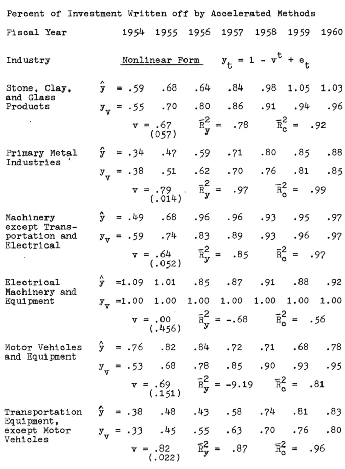
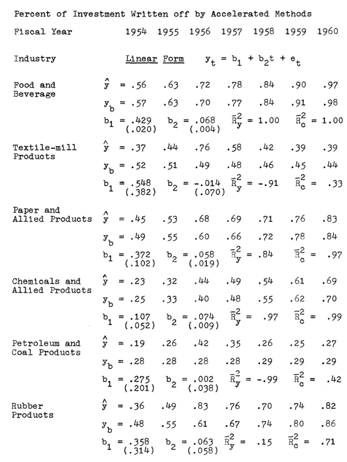
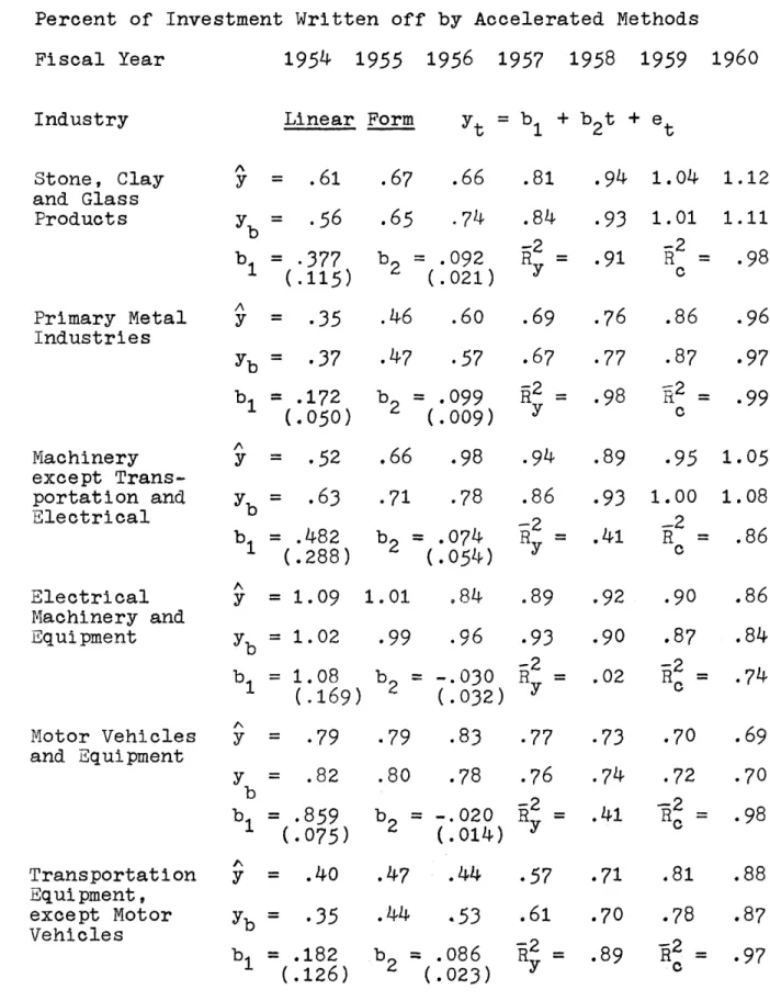
Estimated Depreciation Learning Functions for U. S. Manufacturing Industries
Comparison of Nonlinear Estimates Using Original Asset Lives and Original Lives Increased by Two Years
Error in Effective Depreciation Rates Due to Assuming an Average Asset Life
Regression Results--Investment Equation Regression Results--Investment Equation (Estimated by the Method of Generalized
Least Squares)
Durbin-Watson Statistics for the Original and Transformed Investment Equations--by Quarter 119 121 123 125 126 127 128 129 152 156
157
206 207 208Payout Ratios for Dividend Models 7.6 Regression Results--Dividend Equation
(Intercept and C+GS Excluded) 211 7.7 Regression Results--Debt-Equity Ratio
Equation 212
7.8 Regression Results--External Finance
Equation 213
8.1 Model Test Summary 249
8.2 Percent Change in Investment Due to 1954
Accelerated Depreciation Provisions 250 8.3 Comparison of the Original Investment
Equations with Those Estimated by
General-ized Least Squares 251
8.4 Estimated Potential Increase in Depreciation on Existing Capital Stock Resulting from
1962 Asset Life Reduction 252
8.5 Comparison of 1962 Guideline Depreciation 253 8.6 1962 Investment Credit Statistics 253 8.7 Estimated Effect on Investment of the
1962 Accelerated Depreciation Provisions 254
INTRODUCTION
By accelerated depreciation is meant any change in the timing of depreciation deductions over the life of an asset which results in an increase in the present discounted value (to be denoted pdv) of these deductions. This in-crease of course depends on the discount rate used in cal-culating the present value, and therefore a specific rate or range of rates is required in order to determine what con-stitutes accelerated depreciation. That is, depreciation deductions could be altered in such a manner as to yield an increase in pdv at some discount rates and a decrease at others. For the methods of acceleration which have occurred in practice and to be considered below, however, this is not possible since they all involve increased deductions in
early year(s) with corresponding lower deductions in later years, and the pdv of such a series is greater than zero for all positive discount rates.
Since accelerated depreciation is defined in relative terms, that is, as a change from an existing to a new system, the existing system is itself of importance. The straight line depreciation method (to be denoted SL) is generally considered as the existing system or norm compared to which the methods of double declining balance (DDB) and sum of the
other hand, any of these methods may be taken as the exist-ing system compared to which the introduction of an initial allowance is said to be accelerated. An initial allowance of b percent of cost results in an increased deduction in the first year of b times cost, together with a corresponding decrease in the depreciable base of the asset over the re-maining n-1 years.
Two methods of stimulating investment which have been used in practice but which do not satisfy the above defini-tion of accelerated depreciadefini-tion are the investment credit and reduction in asset life for tax purposes. The former results in a decrease in taxes by the amount of the credit in the first year of an asset's life, but leaves depreciation deductions unchanged. The latter is essentially different because it changes the period over which deductions are
taken. However, it may be thought of in terms of the above definition by considering the new deductions over the longer
life, that is, as deductions of 1/n1 for n1 years and 0 for
lUnder the SL method deductions of 1/n are permitted in each year, for an asset with a life of n years. Under the DDB method the allowable deduction in the kth year of the asset's life is 2/n times the undepreciated value of the asset. Since the latter is given by (1-2/n)k-1, the DDB deduction is (2/n)(1-2/n)k-1. Under the SYD method allow-able depreciation in the kth year is n-(k-1) divided by the sum of the first n digits (n(n+1)/2), and hence equals
2(n-k+1)/(n(n+1)). It should be noted that these expres-sions are given for an asset with unit cost. In the analysis to follow all examples will have this property unless other-wise stated.
n2-ni years, where n is the shorter, n2 the longer life.
For convenience in the work to follow both the credit and re-duction in life are classified as methods of accelerated
depreciation.
The four major methods of acceleration which are therefore to be studied in detail are a switch to SYD, an
initial allowance, an investment credit, and a reduction in asset life for tax purposes. This choice of methods is motivated by recent tax law changes which have resulted in an acceleration of depreciation in practice. The relevant tax provisions are reviewed briefly before consideration is given to the theoretical effects of accelerated depreciation.
Although specific methods of computing depreciation deductions were not specified by the Treasury prior to 1954, methods used were required to be reasonable, to conform with a recognized trade practice, and to be adopted by the tax-payer in his own account. Useful lives for tax purposes were intended to correspond to the length of time assets were retained in use, the life of each asset therefore
depending on the particular circumstances of its employment. Estimated lives contained in Treasury mortality tables, such as Bulletin F, were averages and were not meant to apply to all assets or taxpayers.
The Internal Revenue Code of 1954 specifically author-ized the following three methods of computing depreciation: the straight line method, the declining balance method at not
,
years digits method. Any other consistent method was allowed, provided the deductions at the end of each year during the first two-thirds of the useful life of the property did not result in a greater cumulative deduction than under double declining balance. The option of switching at any time from double declining balance to straight line was permitted in order to recover the total cost of the asset. These methods were applicable to all new assets with a useful life of
three or more years acquired or constructed after December 31, 1953. The 1954 Revenue Code did not include any changes with respect to determination of useful lives for tax pur-poses, although Revenue Ruling 90 issued by the Internal Revenue Service at the time instructed agents not to adjust lives used by taxpayers unless there was a clear basis for change.
New or used property with a useful life of over 5 years acquired after December 31, 1957, was eligible for a
20% initial allowance. The allowance could be claimed on property with a value of not more than $10,000 in any tax-able year.
The 1962 Revenue Act required that entrepreneurs claim a tax credit equal to 7% of qualified investment in new or used machinery bought after December 31, 1961. Qualified Investment was defined as: zero for assets with useful lives of less than 4 years, one-third of cost for
assets with lives greater than
3
and less than 6 years, two-thirds of cost for assets with lives greater than5
and less thar 8 years, and full cost for assets with lives of 8 or more years. The depreciable base of qualified investment had to be reduced by the amount of the credit taken. In any one year the credit was limited to the first $25,000 of tax liability plus one-fourth of any remaining tax liability. Any unused credit could be carried back 3 years and then forward5
years until exhausted.In July, 1962, the I.R.S. published Revenue Procedure 62-61 to replace Bulletin F for the purpose of determining useful lives. Use of the procedure was optional. Useful lives were suggested in general by industry groupings, and by certain Guideline classes that crossed industries such as office furniture and transportation equipment. The Guide-lines were applicable to existing as well as to new facil-ities. The new lives could be used for three years after which they were required to conform with actual lives as
demonstrated by retirement practice. The reserve ratio test was intended to provide an objective basis for determining
if this conformity was met.2 Table 1.1 contains a comparison
2Basically the reserve ratio for each Guideline class is computed by dividing the total depreciation reserves for all assets in that class by their corresponding basis
(including any assets which have been removed from the ac-counts but which are still in use). The reserve ratio cal-culated in this manner must lie in the acceptable range pre-scribed by the Treasury, where the acceptable range depends on the method of depreciation, the Guideline life (n) and the rate of growth of investment over the preceding n years.
in use at the time of introduction of the Guidelines.'s' The Revenue Act of 1964 repealed the provision intro-duced in 1962 which required the depreciable base of assets to be reduced by the amount of tax credit taken. The depreci-able base of assets purchased and subjected to such a reduc-tion in 1962 and 1963 could be increased by a corresponding amount beginning in 1964.
The two major effects of accelerated depreciation, which will be analysed in detail in Chapters 2 and 3, are the
present discounted value and liquidity effects. The former refers to the change in the pdv of a single asset's net revenue stream resulting from an accelerated depreciation provision. That is, when depreciation deductions are in-creased in early years, taxes are reduced and hence net
revenues increased by the amount of the deductions times the corporate tax rate. Of course there is an equivalent de-crease in net revenues in later years, but with a positive discount rate the pdv of these changes is positive. By the pdv effect then is meant the pdv of the change in depreciation deductions times the corporate tax rate, but since the latter
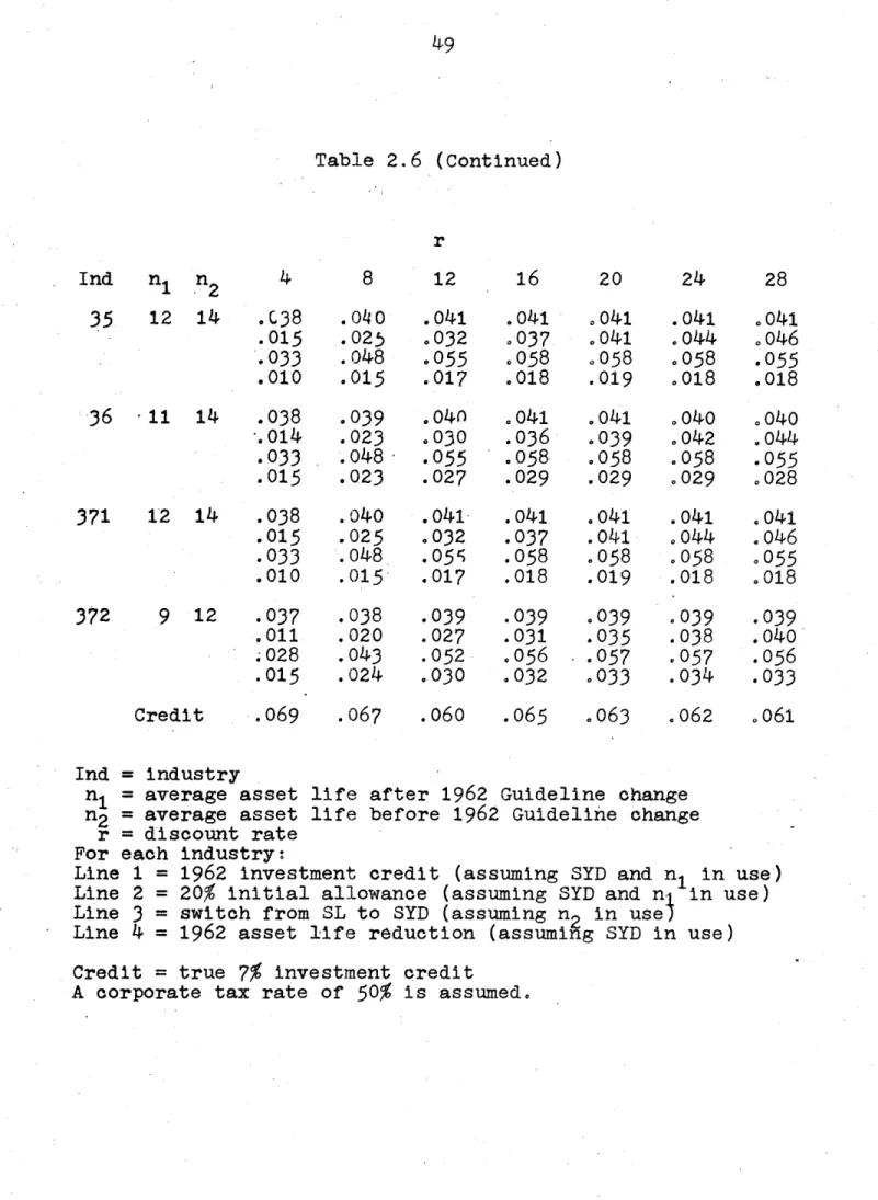
3All numbered tables appear at the end of their respective chapters.
4Table 1.1 also contains for each manufacturing
industry its Standard Industrial Classification number which will be used for reference purposes in the analysis to
is assumed throughout to be constant (at 50%), it is suffici-ent to analyse the former.
There are a number of reasons for analysing changes in pdv. Although the mechanism through which such changes might be expected to result in changes in investment is un-known, a number of hypotheses are possible. First, invest-ment decisions may rest on pdv calculations themselves. Second, investment decisions may be a function of rate of return measures which are affected by pdv changes. Third, the investment process may be formulated in terms of an adjustment process involving a desired capital stock the magnitude of which depends on the pdv of depreciation
deduc-tions (assuming of course a positive corporate tax rate). There exists in the literature on accelerated dep-reciation, a number of studies in which pdv changes are analysed.5 There does not exist, however, a comprehensive analysis of pdv effects such as the one presented in Chapter 2, which allows a comparison to be made of the effects of the major methods of accelerated depreciation over a wide range
5See
for example, E. C. Brown, "The New Depreciation Policy Under the Income Tax- An Economic Analysis", National Tax Journal, March, 1955, in which the effect on pdv of a switch from SL to SYD is studied; and M. M. Dryden, "Capital Budgeting and the Investment Credit", Working Paper 24-63, School of Industrial Management, M.I.T., June, 1963, inwhich the pdv change resulting from the 1962 credit is anal-ysed. Other relevant works include Richard Goode, "Acceler-ated Depreciation Allowances as a Stimulus to Investment",
Q.J.E., Vol. LXIX (May, 1955), pp. 191-220 and George Terborgh, Realistic Depreciation Policy, M.A.P.I., 1954.
cause it is very difficult in the absence of such a compari-son to determine the relative incentive to investment pro-vided by the different methods. The effect on pdv changes of variations in the discount rate and asset life can also be analysed, and is of interest in discovering the relative
incentive provided to assets with different lives and of different degrees of riskiness. The latter is possible to the extent that the discount rate may be interpreted as a measure inclusive of risk. Finally a table is presented which allows a direct comparison to be made of the effects of the 1954 and 1962 provisions, for asset lives which are intended to approximate the average lives used in the two-digit manufacturing industries,
The second major effect of accelerated depreciation is the liquidity effect. The liquidity measure to be con-sAdered is the ratio of total depreciation deductions to total investment.6 This ratio gives the fraction of invest-ment in any period which can be financed internally from depreciation allowances, Such a concept is of interest if there exists an advantage to financing investment internally. The nature of this advantage will be discussed in Chapter 4.
Of course total cash flow consists of net profits as well as depreciation allowances, and an increase in the
6
This terminology differs from standard usage in that the liquidity measure defined here is a flow rather than a
latter due to accelerated cepreciation will reduce taxable and hence net profits. It is not hard to show, however, that cash flow will increase by the tax rate times the change in depreciation deductions. Consider the following simplified identity in which D is depreciation, Pn is net profit, Pg is taxable profits less all deductions except depreciation, and T is the corporate tax rate, then Pn = g-D)(1-T). Cash flow (CF), which equals Pn+D, is therefore given by
CF
=
(Pg.D)(1-T) + D or CF = Pg(1-T) + DT, which shows that an increase in depreciation deductions, ceteris paribus,increases cash flow by the tax rate times the change in deductions. This increase in cash flow is an upper bound to the amount (depending on the fraction of profits retained) by which the internal financing of investment can increase as a result of accelerated depreciation. Since this increase is given by a constant (the tax rate) times the change in depreciation deductions, it is sufficient to concentrate on the latter in order to determine the effect on internal financing.
In analysing the effect of accelerated depreciation on liquidity it is necessary to distinguish between the case of a single asset and that of a stream of assets. This
distinction is not necessary for pdv analysis, but liquidity analysis is relevant only in the context of a stream of
assets. That is, the variable of interest in any period is the ratio of total depreciation to current investment where
ferent times in the past. For a single asset of course the behaviour of the depreciation-investment ratio over time is simply given by the depreciation rate itself, and any in-crease in deductions in early years by definition equals the decrease in later years. But for a stream of assets the total depreciation deduction in any period is a function of investment expenditures over the preceding n years, where n is the average asset life. In order to determine the total depreciation deduction then it is necessary to make an
assumption about the past growth of investment. For a posi-tive growth rate, the increase in deductions on new or
recent assets due to accelerated depreciation will not equal the decrease on older assets, because the stock of newer assets is permanently larger.
There exists in the literature a number of studies in which the advantages to be gained from accelerated depre-ciation under conditions of growth are recognized. Probably the first authors to explicitly analyse the time path of deductions for different methods for a stream of growing assets were R. Eisner and E. D. Domar.7 The former showed that with a positive growth rate of investment, the aggregate
7
Robert Eisner, "Accelerated Amortization, Growth, and Net Profits", Q.JE., Vol. LXVI (November, 1952), pp. 533-544; and Evsey D. Domar, "The Case for Accelerated Depreci-ation", Q.J.E., Vol. LXVII (November, 1953) pp. 493-519.
depreciation-investment ratio would increase as the length of asset life decreased, under the SL method. To illustrate the effect, hypothetical depreciation values were calculated for the U. S. economy using actual investment figures but assuming different SL amortization periods.
E. D. Domar studied the behaviour of the ratio of accelerated to normal depreciation under conditions of an exponential growth rate of investment and no initial capital stock. The methods of accelerated depreciation studied were the combinations of DDB and an initial allowance, SL and an allowance, and SL with a shorter life. Advantages accruing to new and growing firms were emphasized. But Domarts con-clusions (which have essentially become the commonly held views in the literature) rest entirely on the assumption that the most appropriate measure of advantage from accelerated depreciation is the ratio of accelerated to normal deductions. One important implication of such an assumption, for any of the methods of acceleration studied here or in Domar's work, is that the gain from acceleration will decrease (or remain constant) during transition to steady state conditions. It will be argued below that the difference of depreciation deductions rather than the ratio of such deductions is a more suitable measure of the advantage from acceleration, in which case some of Domar's conclusions, and in particular the one just noted, must be modified.
A detailed account of the literature on the subject of depreciation dedictions under conditions of growth will
however, would include E. C. Brown, E. D. Domar, R. Eisner, and R. Goode.8 In spite of the substantial number of articles relating to the behaviour of depreciation deductions under conditions of growth, there exists neither a comprehensive study nor one in which the relation to liquidity factors is clearly stated. The analysis to be presented in Chapter 3
may be considered comprehensive for the following reasons. It allows a comparison to be made of the effects of the vari-ous major methods of accelerated depreciation, as well as of different asset lives, growth rates, and types of growth. The transitional effects for growing firms are studied
care-fully since their relevance for n years (the average asset life) after introduction of the new methods makes them important. Steady state depreciation to investment ratios are analysed and shown to be equivalent to pdv expressions when the growth rate is interpreted as a discount rate. Finally, the relevance of the change in the depreciation-investment ratio resulting from accelerated depreciation is studied in terms of the advantages to be gained from the increased capability to finance investment internally.
The analysis of the liquidity and pdv effects outlined and presented in detail in Chapters 2 and
3
is straightfor-ward in that it simply involves computing changes in the8See Brown, op. cite, Domar, op. cit., Eisner, op. cit.,
relevant parameters. A much more difficult problem is to determine the manner in which and the extent to which these
changes affect investment decisions. Such a step is of course necessary for an empirical determination of the im-portance of the 1954 and 1962 Revenue Act provisions. If perfect rationality could be attributed to all entrepreneurs and if the exaqt manner of reaching investment decisions were known, then the pdv and liquidity factors, which theor-etically should affect investment, could be translated into actual changes in investment. However, neither of these assumptions is acceptable. First, entrepreneurs do not always follow objectively rational practices when making
investment decisions, whether because subjective preferences are considered more important, or because of ignorance of appropriate methods. Second, there exists in the literature a wide variety of determinants which are hypothesized to affect investment (to varying degrees) while attempts to describe investment behaviour econometrically have not re-sulted in general acceptance of any particular subset of these.
An assumption must be made therefore about the factors which determine investment decisions in order to investigate the effect of accelerated depreciation on them and hence on investment. If these factors are influenced by pdv and liquidity considerations then their incorporation (if pos-sible) into an empirical model provides a means for
14
determining empirically the effects of depreciation changes. Two points should be mentioned. First, even if pdv and
liquidity changes do affect investment decisions it may be possible to argue, in view of the orders of magnitude of such changes, and in view of the probably rough predictions of future revenues and costs required in making investment deci-sions, that one or both of the effects is essentially neglig-ible. Second, since investment decisions may be based on not entirely rational grounds, some mechanism may exist through which accelerated depreciation affects investment other than the two mentioned above.
In order to gain further insight into the factors which are considered important by entrepreneurs in reaching investment decisions, a brief report on two recent interview studies of corporation executives is given in Chapter 4. Attention centers on rate of return measures used by entre-preneurs in analysing investment projects, and particular emphasis is placed on determining whether such measures are affected in general by accelerated depreciation. (The extent
to which such measures are affected is analysed in Chapter 5.)
In view of the fact that accelerated depreciation re-sults in a permanent increase in liquidity (for growing firms), Chapter 4 also contains an analysis of the advantages of
financing expenditures from internal sources, and a descrip-tion of the extent to which this practice is followed. Aside from rational reasons for preferring internal funds, probably
the major one of which is due to differences in tax rates on dividends and capital gains, entrepreneurs exhibit a strong subjective preference for them which in some cases may not be entirely rational. Whether for rational reasons
or not, however, the existence of such a preference suggests that the liquidity effects resulting from accelerated
depreciation may well be important.
Chapter
5
contains a comprehensive investigation of the orders of magnitude involved in rate of return changes resulting from specific accelerated depreciation provisions. In spite of the fact that the elasticity of investment with respect to such changes will in general be unknown, there are at least two reasons for analysing them. First, they are of interest in comparing the different methods of accel-erated depreciation, and in comparing variations in asset lives and initial rates of return. Second, the orders of magnitude involved are of interest. In particular, ifacceleration results in very small changes in rate of return measures, one might be justified in assuming their influence on investment negligible in view of the roughness with which such measures are likely to be constructed, being based on revenue predictions over the asset's entire life.
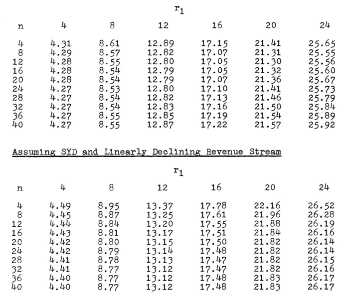
There exists in the literature a scattered discussion of changes in rate of return measures resulting from accel-erated depreciation. In particular analysis has centered on the internal rate of return. G. Terborgh has calculated the
assuming an initial internal rate of return of 10% and a
9
linearly declining revenue stream. M. Dryden has tabulated the effect of the 1962 investment credit for various initial internal rates and with a linearly declining revenue stream, and has experimented slightly with the revenue stream
assumption.10 There exists, however, no comprehensive
analysis of rate of return changes such as the one presented in Chapter 5. The effects on the internal rate of return for various initial rates and asset lives, and under the assumptions of constant and linearly declining revenue
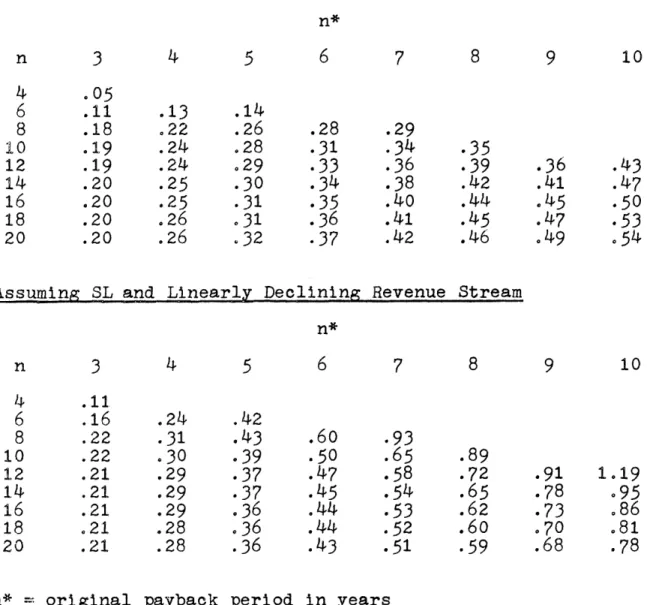
streams are given for the four major methods of accelerated depreciation mentioned above. The effects on a modified internal rate of return, which avoids the assumption of reinvestment at the internal rate, are also given. Finally in view of the reportedly widespread use of such a rate of return measure, the change in an asset's payout period due to accelerated depreciation is analysed.
It is important to recognize the relation between the pdv and liquidity effects discussed in Chapters 2 and 3, and
9George Terborgh, Incentive Value of the Investment
Credit, the Guideline Depreciation System, and the Corporate Rate Reduction, M.A.P.I., Washington, D. C., 1964; and New Investment Incentives, M.A.P.I., Washington, D. C., 1962.
10Miles M. Dryden, "How do Recent Changes in Tax Laws Affect Investment Decisions?" Working Paper 25-63, School of Industrial Management, M.I.T., June, 1963.
the rate of return analysis in Chapter
5.
The changes in the internal rate of return and the modified rate of returnconsidered in Chapter
5
are essentially pdv changes trans-lated into rate of return terms. That is, such changes arise because of variations in the timing of an asset's (discounted) depreciation deductions, although the total amount of deduc-tions remains the same. For the internal rate of return, depreciation deductions are discounted at the internal rate(whatever it may be), while for the modified internal rate deductions are discounted at the firm's cost of capital.
Variations in an asset's payout period due to acceler-ated depreciation do not depend on the pdv or the liquidity effects as defined above. That is, since discounting is ignored the effect is not one of present values, not is it concerned with the effect on the aggregate depreciation-investment ratio of a stream of assets. Rather accelerated depreciation alters an asset's payout period simply by
increasing net revenues in early years thereby reducing the period of time taken for revenues to accumulate to invest-ment cost. The payout period is strictly speaking not a
rational profitability measure, and hence is not included in the analysis in Chapters 2 and
3
of the two major effects of accelerated depreciation. It is included in the discus-sion on rate of return measures because of its reportedly widespread use in practice.No account is taken in the rate of return calculations in Chapter 5 of the liquidity effect considered in Chapter 3.
in a single asset's revenue stream resulting from accelerated depreciation, while the liquidity factor as defined above is relevant only for a stream of assets. These two concepts, may be related however, in the following manner. Since the liquidity effect in any period after introduction of acceler-ation reduces the cost of financing investment by allowing more to be financed internally, then it results effectively in an increase in the rate of return of each asset purchased in that period. That is, the cost of financing each asset may be considered reduced and hence its rate of return in-creased. The reduction in cost will depend not only on the extent of the increase in internal financing made possible by the acceleration, but also on the importance of this
in-crease to the firm. The former is exactly what is analysed in Chapter
3
under the heading of the liquidity effect and depends therefore on the average asset's life and the growth rate of investment. The importance of this increase to the firm, however, is not readily determinable because it depends on the subjective preference of the firm for internal funds, as well as on the relative costs of internal and external funds. For this reason no attempt is made to translate liquidity changes into rate of return changes, and in the rate of return analysis presented in Chapter5
financing costs are assumed constant.In contrast to the many discussions which exist in the literature on the theoretical effects of accelerated
depreciation on investment, empirical analyses are almost nonexistent. The author is aware of only two (as yet un-published) papers in which an attempt is made to determine empirically the effects of accelerated depreciation. The first is a paper by R. E. Hall and D. W. Jorgenson. The second is a Doctoral Dissertation by R. M. Coen. The analyses are very similar in that they both assume that
investment expenditures depend on the difference between the existing capital stock and a desired capital stock. The latter is made a function of the "user cost" of capital, and this cost in turn depends on the pdv of depreciation deduc-tions earned by the assets involved (assuming a positive corporate tax rate of course). A change in the pattern of such deductions therefore changes their present discounted value, and hence the desired and actual capital stocks.
(This alleged direct dependence of investment expenditures on the discounted value of depreciation deductions provides additional motivation for the pdv analysis of the next
chapter.)
Probably the major reason for the lack of empirical work in this field is the fact that any such analysis will of necessity depend crucially on the nature of the investment
11R. E. Hall and D. W. Jorgenson, "Tax Policy and
Investment Behaviour", 1966, (to be published in the A.E.R.), and R. M. Coen, Accelerated Depreciation, The Investment Tax Credit, and Investment Decisions, (Preliminary), Unpublished Manuscript, December, 1965.
function
rely entirely on the assumption that investment expenditures respond (in a specified manner) to changes in the present discounted value of depreciation deductions earned on fixed assets. This means that entrepreneurs must employ precise discounting procedures, or act as if they did, when making investment decisions. If entrepreneurs do not in general use discounting methods, another formulation of investment behaviour might be more appropriate. The real problem then lies in the fact that, as mentioned above, a wide variety of determinants are hypothesized to affect investment while attempts to describe investment behaviour econometrically have not resulted in the general acceptance of any particular investment function.
The model of investment behaviour hypothesized in this paper and studied in detail in Chapter 7 is oriented more towards the profit models in the literature than towards the Jorgenson capital model as outlined above. The assumption is made that the firm's cash flow (depreciation plus net profits) plays a major role in influencing investment decisions. The mativation for making such an assumption is the preference
(some reasons for which are discussed in Chapter 4) of entre-preneurs for internal funds. Pressure on capacity, the
availability of eXternal funds, and the current liquid posi-tion of the firm are also assumed to affect investment.
The investment equation is postulated to be one of a system of equations that involves a simultaneous determination
of investment, dividend, and external finance behaviour. Dividend and investment expenditures both rely heavily on cash flow, which in turn depends on investment due to its depreciation component. The level of external finance is affected by investment opportunities relative to the supply of internal funds, while investment itself is influenced by the availability of external finance. The budget constraint of the firm requires that these decisions be consistent.
Dividend behaviour in general is assumed to follow the basic Lintner model in whieh the change in dividends in any period represents partial adjustment towards a desired level of dividends, with the latter being a constant fraction of cash flow. Variations from this pattern may result due to differences in the liquid position of the firm. The cash flow variable is used rather than net profits in view of recent findings by several authors which suggest that cash flow is the superior income variable.1 3 By far the most
12John K. Lintner, "Distribution of Incomes of Corpor-ations Among Dividends, Retained Earnings, and Taxes",
Proceedings co the American Economic Review, Vol. 46, No. 2, (May, 1956) pp. 97 -113.
1
3.See
in particular John A Brittain, CorporateDivi-dend Policy The Impact of the Tax Structure and Other Factors, (Preliminary Manuscript), March, 1965; R. Sutch,
ISoe Comments on Corporate Dividend Behaviour", Unpublished Manuscript, January, 1966; R. Gordon, "Explaining Corporate
Payout Behaviour"1 , Unpublished Manuscript, July, 1965, and E. Kuh, "Income Distribution over the Business Cycle", Chapter 8 of The Brookins Quarterly Econometric Model of the United States, Chicago, 1965, pp. 275-278.
Brittain, whose basic behavioural hypothesis is that firms are aware of the depressing effect of changing depreciation provisions on their ability to pay dividends, and will take this into account when making such payments. Three arguments are offered in support of the proposition. First, firms may think of depreciation as a purely accounting charge in which case cash flow will be viewed as one source of funds to be distributed between dividends and investment. Second, firms may regard stability of dividends more important than invest-ment expenditures, and consequently finance dividends direct-ly from cash flow. Finaldirect-ly, in a period of changing depreci-ation reguldepreci-ations firms will desire to utilize consistent depreciation rules for determing dividend payments, and for
simplicity may use cash flow as an approximation.
The external finance behaviour of firms is analysed in considerable detail. Such behaviour is assumed to depend not only on current investment expenditure and the supply of internal funds but also on the cost of financing externally, the firm's current liquid position, and the relation of long term debt to equity. The latter assumes that borrowing
decisions are influenced by the difference between an optimal and the actual debt-equity ratio. An attempt is made to
determine whether the resort to outside funds is best repre-sented by past, current, or future expectations of investment expenditure, and to determine if it depends in a nonlinear
fashion on financing needs. The major components of external finance, long term bank borrowing and corporate bond issues, are analysed separately in an attempt to determine the extent to which their determinants differ.
in a recent book by W. H. Locke Anderson an attempt is made to explain investment in fixed assets, short and long term borrowing, and the accumulation of cash and government securities.1 4 The analysis is based on quarterly time series data for the two-digit manufacturing industries. A major drawback of the study is its failure to allow for simultane-ity in the estimation procedure while stressing the inter-dependence of financial decisions in the theoretical discus-, sion.
The author is aware of only one other study in the literature in which a simultaneous model of investment, dividend, and external finance behaviour is statistically estimated. It is a recent paper by P. J. Dhrymes and M. Kurz
involving a cross section analysis similar in some respects to the time series analysis presented here.15
The reduced form of such a system of equations may be used to determine the effect of any method of accelerated
14W. H. Locke Anderson, Corporate Finance and Fixed Investment, Boston, 1964.
15Phoebus J. Dhrymes and Mordecai Kurz, Investment,
Dividend and External Finance Behaviour of Firms, (Preliminary), presented at the Conference on Investment Behaviour,
spon-sored by Universities-National Bureau Committee for Economic Research, June 10-12, 1965.
1954 and 1962 Revenue Acts. The mechanism through which accelerated depreciation affects the endogenous variables is of course by changing the pattern of depreciation deductions, and therefore cash flow, over time. Variations in cash flow result in variations in dividend payments, the level of
external finance, and investment expenditures, with the latter feeding back onto cash flow through a further change in depreciation deductions. Using an initial set of lagged endogenous variables and the actual values of exogenous
variables, the reduced form can be used to generate values of endogenous variables which are functions of any desired
accelerated depreciation parameter.
The following identity (in simplified form) contains the depreciation parameters which can be altered in order to analyse the different methods.
Dt = Dt-1 + vt t + Ct + Rt
Dt is depreciation, vt is the depreciation rate applied
against current investment, Ct is a correction term which is required if the depreciation method results in unequal deduc-tions over time, (and is therefore required for all methods but SL), and Rt is current retirements of fixed assets. By appropriately adjusting Ct and vt and then using the reduced form to generate values of endogenous variables, any method of accelerated depreciation may be analysed. For example, if SYD were used instead of SL, then basically vt would be
2(n-k+1)/n(n+1) rather than 1/n, and Ct would have to be
adjusted to take into account the fact that under SYD deduc.-tions on any asset decrease by an amount equal to 2/n(n+1) each year. A reduction in asset life for tax purposes from n2 to n1 would require that n, be used instead of n2 in
computing vt and Ct. This general method of analysis is used in Chapter 8 in an attempt to determine the effects of the liberalized depreciation provisions introduced in 1954 and 1962.
A major problem in determining the effect of the introduction of accelerated methods in 1954 arises in con-nection with the fact that entrepreneurs did not immediately accept such methods but adopted them only slowly over the years. A problem arises because there is no direct infor-mation available on the extent of use of the accelerated methods by two-digit industry, nor is the author aware of any estimates of their use. Clearly information on the rate of adoption is required as a part of the parameter vt in
the depreciation identity given above. That is, in analysing a switch from SL to SYD, vt will be a weighted average of the two depreciation rates, with weights equal to the amounts of investment written off under the two methods.
For this reason an attempt is made in Chapter 6 to
estimate an adoption rate or learning function for accelerated depreciation. Satisfactory results are obtained for all
industry, there is in the case of the petroleum industry, in that depletion provisions may make accelerated depreciation less advantageous than straight line. The statistical
techniques derived and used in obtaining learning function estimates have not, to the author's knowledge, appeared in the literature.
Before turning to the analysis of pdv effects in the next chapter, a few details will be given concerning the different methods of accelerated depreciation.
As mentioned above, DDB results in a deduction in year k of an asset's life of an amount equal to (2/n)(1-2/n)k-1. Since (2/n)(1-2/n)k-1= 1 - (1-2/n)n it is clear that at the end of n years the asset will not be completely depreci-ated. For this reason the law permits a switch from DDB to SL at any time during the asset's life. Profit maximization requires a switch when the annual deductions under the two methods are equal, and for an asset with life n this occurs
in year n/2+1, calculated as follows. The percent of cost written off after t years is given by
Z(
2/n)(1-2/n)k-11-(1.2/n)t, leaving (1-2/n)t for later years. The switch occurs in year k+1 determined by equating deductions: (1-2/n)k/(n-k) = (2/n)(1-2/n)k, from which k+1 = n/2+1.
If complete rationality is not assumed and switching does not occur, it can be shown that for certain values .of the discount rate (r) and asset life (n), the SL method
results in a higher present discounted value of deductions than the DDB method. That is, by solving for the value of r which equates deductions under the two methods for a given n, one obtains the discount rate below which the present value of the deductions using SL exceeds that of DDB. For asset lives of 5, 10, 15, 20 and 25 years respectively the critical discount rate is approximately given by 9, 7, 5, 4, and 3%. Such calculations illustrate the crucial role of the discount rate in the definition of accelerated depreci-ation.
The pdv and liquidity computations under DDB are complicated if switching is assumed, and the problem men-tioned above is encountered if it is not. For this reason, the SYD method of depreciation is used in the analysis in Chapters 2, 3, and 4 to represent both the accelerated
methods (DDB and SYD) introduced in 1954. The error involved in using SYD in place of DDB is small, since the two methods
(assuming switching) result in essentially the same pattern of deductions.
An initial allowance, which results in a larger deduc-tion in the first year with an equal reducdeduc-tion in later years, is more beneficial under SL than SYD or DDB. This follows (for n > 2) because, although the gain is always taken in the first year, the write-down of the base occurs closer to the present using an accelerated method. For n=2 there is no difference since the remainder of the asset is completely
combination of SYD or DDB and an allowance remains preferable to SL and an allowance.
The continuous formulations of the three methods of depreciation are used to some extent in the analysis in
order to simplify the mathematics. The SYD rate is the only one in which a change is evident, since the SL and DDB rates remain as 1/n and 2/n(1-2/n)k respectively. The continuous SYD rate applicable at time k of an asset's life is given by 2(n-k)/n 2 and since 2(n-.k)/n 2dk = 1, the asset is complete-ly depreciated as required.
In practice the depreciable base of an asset must -be reduced by its estimated salvage value before applying the SL or SYD methods, but not the DDB method. Since there is little to be gained in the theoretical discussions from assuming varying amounts of salvage (in relation to cost), and since no relevant data exist for the empirical work,
Table 1.1
COMPARISON OF 1962 GUIDELINE LIVES AND AVERAGE LIVES USED IN PRACTICE (1962)
Industry Industry Current Guideline
Description Number Lives Lives
Food and Beverage 20 15 13
Textile-mill Products 22 16 13
Paper and Allied 26 19 15
Products
Chemicals and Allied 28 13 11
Products
Petroleum and Coal 29 18 15
Products
Rubber Products 30 14 13
Stone, Clay, and 32 18 16
Glass Products
Primary Metal 33 21 17
Industries
Machinery except Trans- 35 14 12
portation and Electrical
Electrical Machinery 36 14 11
and Equipment
Motor Vehicles and 371 14 12
Equipment
Transportation Equipment 372 12 9
Except Motor Vehicles
Source: Based on asset lives in the Treasury Depreciation Survey, Treasury Department, Office of Tax Analysis,
November, 1961, Table 1, (Unpublished), and Depreciation Guidelines and Rules, (Revenue Procedure 62-61), U.S.
Treasury Department, I.R.S., Publication No. 456, Revised, August, 1964, pp. 6-13. For any industry in which more
than one Guideline life appears in Revenue Procedure 62-61 the entry in Table 1.1 is a weighted average (using 1962
investment values) of these lives. All asset lives have been rounded to the nearest integer.
PRESENT DISCOUNTED VALUES
As mentioned in Chapter 1 the two major effects of accelerated depreciation are the pdv and liquidity effects. The purpose of this chapter is to analyse the former. The
four basic methods of accelerated depreciation to be considered are: a switch from SL to SYD, the introduction of an initial allowance, the introduction of an investment credit, and the adoption of a shorter asset life for tax purposes. As men-tioned above reasons for making such calculations rest on the assumption that investment is affected by pdv changes. Al-though the precise elasticity of investment with respect to such changes may be unknown, the calculations are of interest in that when combined with order of magnitude elasticity
estimates, they provide some idea of the orders of magnitude involved. A comparison of incentives across methods as well as for different asset lives and interest rates is also of
interest.
It should be recalled that the pdv analysis in this chapter is concerned with a single asset while the liquidity analysis in the next chapter involves a (constant or growing) stream of assets.
The Effect on PDV of a Switch from SL to SYD
Let n be the tax life of an asset and r the rate at which deductions are discounted. The change in net revenue
in any period from using SYD instead of SL equals the change in depreciation deduction for that period times the corporate tax rate. Discounting these changes by the rate r and summing gives the change in present discounted value. Assuming SL and continuous discounting, the present value of depreciation deductions is given by:
PDV(SL) = e-rt/n dt
0
and under SYD the corresponding expression is: PDV(SYD)
j
(2(n-t)/n2)e-rtdt.Let y = PDV(SYD)-PDV(SL), then ys times the corporate tax rate is the gain in discounted value from using SYD. Table 2.1 gives values of ys for selected r and n.1
From the table it can be seen that ys is neither a monotonic function of r for fixed n, nor of n for fixed r. Considering ys first as a function of r only, the introduc-tion of SYD increases the present value of early deducintroduc-tions and decreases the value of later ones. A higher discount rate reduces both early and late deductions. The discount rate for which the gain in deductions is a maximum is there-fore the one for which a higher rate reduces near deductions more than it reduces future ones. For each n this value of r
can be calculated by setting the partial derivative of ys with respect to r equal to zero, and solving to obtain r. Table 2.2 contains such values of r for n less than 40 years, although
1Unless otherwise stated all such tabulations of changes resulting from an acceleration of depreciation are based on annual rather than continuous discounting.
From the fact that ys declines for large values of r the conclusion is often drawn that the benefits from
switch-ing to SYD decrease for risky assets. That is, the discount rate in the preceding calculations may be thought of as play--ing a dual role -- that of discounting for time per se and for risk. A time discount rate is applied because revenues are received in the future. If uncertainty is involved in the outcome a risk discount factor may be applied as well. Gener--ally the latter will be an increasing function of time since more risk is associated with distant revenues, either because of greater probability of not receiving them or they are pre-dicted with less certainty. One plausiie manner in which to discount for risk is to discount revenues in year t by (1+r)t thus resulting in a discounted value calculation of the usual sort. but since there are an infinite number of ways to dis-count, each ctepending on predictions about the future, differ-ent conclusions from those based on Tables 2.1 and 2.2 might be reached.
Even if the particular assumption that revenues in pe-riod t are discounted for risk by (1+r) is accepted, care must be taken in interpreting Tables 2.1 and 2.2 since the discount rate appearing in the tables combines both the time and risk factors. Let r1 be the time, and r2 the risk discount
2For simplicity it is assumed (although perhaps
un-realistically) that the same risk discount rate is applied to gross revenues as to depreciation deductions.
rate, then r in Tables 2.1 and 242 is related to these two rates by the following equation:
(2.1) (1+r) = (1+rI)(1+r
2)
This means that the risk discount rates for which the benefits from accelerated depreciation are a maximum are considerably less than the values given in Table 2.2. For example since YS for n = 20 reaches a maximum at r = .13, then for a time discount rate of .05, the risk discount rate (r2 ) which maximizes pdv may be calculated as:
(1+r2)(1'05) = 113 or r2 = .076
In conclusion, if risk is associated with discounting revenues in period t by (1+r 2)t then for any given asset life (n) and time discount rate (r 1 ) there exists a value of the risk discount rate r*, above which the gain from accelerated depreciation decreases. Using Table 2.2 and equation (2.1)
it can be seen that for large n and a high time discount rate, r2 may well equal zero. If this is the case, any discount for risk decreases the benefit derived from accelerated dep-reciation, and the maximum incentive is for investment in riskless assets.
If ys is considered as a function of n only, an
analysis of the same form as above would reveal for any r, the n which maxi-mizes the gain. This has not been done but an idea of the orders of magnitude involved can be obtained from Table 2.1. For example, discount rates of .16 and .24 yield the maximum advantage for assets with lives of approximately 20 and 16 years respectively.
Present value calculations for a change from SL to DDB (assuming the switching provision is used) are not pre-sented but it is clear that the results will be similar to those given in Table 2.1. On the other hand, as stated in the preceding chapter, if DDB is used ignoring the switching provision then for low discount rates the SL method will have a higher pdv than the DDB method.
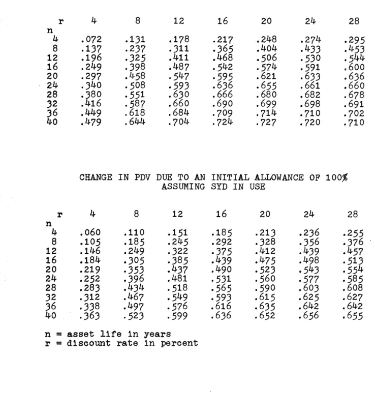
The Effect on PDV of an Initial Allowance
As mentioned in Chapter 1, the introduction of an initial allowance is more beneficial if SL rather than an accelerated method such as SYD is in use. An initial allow-ance of b% of cost results in a gain in deductions in the
first year of b, with a corresponding loss of b over the remaining n-1 years. The discounted value of the net gain from introducing the allowance, assuming SL is in use (and before multiplying by the tax rate) is therefore given by:
ya (SL) = b e-rtdt- bfert/(n-1) dt The corresponding expression assuming SYD is:
n
ya(SYD) = bf e-rtdt - b (2(n-t)/(n-1)2 )e-rtdt
0 1
Note that the loss of b in deductions is spread over n-i years in proportion to a depreciation rate applicable to an asset of n-1 years. For this reason 1/(n-1) is the SL rate in the second part of ya(SL) and ((n-1)-(t-1))/(n-1)2 is the corresponding SYD rate. Values of ya(SL) and ya(SYD) appear in Table 2.3 for b = 100% and selected r and n. In order to , compare the effects resulting from an allowance with other
m'ultiplied by the value of the allowance.
A prjori one would expect the gain from using the
allowance to follow the same pattern with respect to the dis-count rate as the gain from using SYD in place of SL. That is, for a given asset life the gain should increase with r at first and then decrease. Table 2.3 shows this to be the case, although the effect is not very pronounced because the only year with increased deductions is the first.
With respect to asset lives, however, there is a basic difference between the gain resulting from an initial ance and that from a switch to SYD. In the case of an allow-ance, the net gain increases monotonically with n for any acceptable depreciation allowance (defined below). This proposition is not difficult to prove.
Let ya = the increase in pdv resulting from an initial allowance
b = initial allowance as a percent of cost r = discount rate
n = asset life
T = corporate tax rate
h(t,n) = depreciation deduction on an asset of age t with life n. h(tn) must satisfy the following condi-tions for all n> 0.
(a) h(t,n)>0 for 0,<t6 n = 0 for t >n (b) h(t,n) dt = 1
Condition (a) states that all deductions over the asset's life must be positive, (b) requires that the total deduction be equal to cost, and (c) requires that the deduction in any year be smaller (or the same) for a longer lived asset.
ya is therefore given by:
(2.2) ya = bT e rtdt - bT h(t-1,n-1)ertdt and differentiating ya with respect to n gives:
(2.3) dya/dn = -bT(h(n-1,n-1)e-rn + rt Jd/dn (h(t-1,n-1))e- dt
From condition (b) above, h(t-1,n-1)dt = 1 and differenti-ating with respect to n gives:
h(n-1,n-1) + d/dn(h(t-1,n-1)) dt = 0 Substituting for h(n-1,n-1) in (2.3) yields:
(2.4) dy/dn = -bT( (d/dn(h(t-1,n-1)))(e-rt- e-rn)dt) But e-rt_ e-rn>O for t = Jn and d/dn(h(t-1,n-1)),<0 from condition (c). Therefore the integral in (2.4) is negative since it consists of all negative terms, and hence dya/dn itself is positive.
This shows that the gain from an initial allowance is an increasing function of n, which is a plausible result if the allowance is thought of as an interest free loan in the first year, to be paid back over the life of the asset. The longer the life the more benefit is obtained. A switch from SL to SYD can not be thought .of in these terms because the period during which the loan occurs is not restricted to the first year, but varies with the asset life.
the gain from an allowance, as a function of r, increases at first and then decreases. Differentiating ya with respect to r gives: dya/dr = -(bT/r)I e-rttdt + (bT/r) fh(t,n)e-rttdt
0
Since the second term is positive, dya/dr would be positive if it were not for the fact that the gain is taken over the first period and must be discounted. For small r the -first period discounting will be unimportant and dya/dr will be positive, but for large r the first term will dominate. This shows that for all depreciation functions h(tn) the
gain from an initial allowance increases at first, but de-creases for r greater than some r*, which depends on h(t,n). The Effect on PDV of an Investment Credit
The change in discounted value resulting from an
investment credit is simply the amount of credit k discounted by r over the first period, that is, k e-rtdt. This value decreases with r and is independent of n and the corporate tax rate.
The investment credit introduced in the 1962 Revenue Act consists of a 7% tax credit in the first period together with a write-down of the base over the asset's life. The required write-down of the base means that the pdv of the credit will depend on the asset's life and the corporate tax rate. The gain in pdv resulting from such a credit is given by: yk = *07 e-rtdt - ,07T h(t,n)e-rtdt
0
As with an initial allowance dyk/dn> 0 for all n but dyk/dr> 0 only for r less than some r *.
from the 1962 credit for various asset lives and discount rates. Since the credit is applicable only to machinery and equipment,asset lives greater than 24 years are not presented. The required reduction in credit for lives of less than 8
years is taken into account in the calculations. The table indicates that credit is more beneficial for assets with long lives and if SL rather than SYD is in use. The absolute gain does not appear to vary much with the discount rate, but the pattern of increase followed by decrease, as r increases is discernible.
The Effect on PDV of a Change in Asset Life
Let n1 be the new shorter asset life for tax purposes, and n2 the old life, Then the increase in pdv due to using the shorter tax life is the difference between the depreciation deductions under the two lives. This increase in pdv may
also be thought of as resulting from a change in deductions of h(t,n 1 )-h(t,n2 ) in the first nj years and of -h(t,n2 ) in
the remaining n2-n1 years, where h(t,n) is the depreciation deduction on an asset of age t with life n. The increase in
pdv is then:
y
5
(h(t,nl)-h(t,n2)e -rtdt - h(t,n2 )e-rtdt 0= h(t,nl)ertdt -
f
h(t,n2)ertdt0
which shows that y. equals the difference between depreciation deductions'under the two lives.