HAL Id: hal-00295440
https://hal.archives-ouvertes.fr/hal-00295440
Submitted on 24 May 2004
HAL is a multi-disciplinary open access
archive for the deposit and dissemination of
sci-entific research documents, whether they are
pub-lished or not. The documents may come from
teaching and research institutions in France or
abroad, or from public or private research centers.
L’archive ouverte pluridisciplinaire HAL, est
destinée au dépôt et à la diffusion de documents
scientifiques de niveau recherche, publiés ou non,
émanant des établissements d’enseignement et de
recherche français ou étrangers, des laboratoires
publics ou privés.
Temperature lidar measurements from 1 to 105 km
altitude using resonance, Rayleigh, and Rotational
Raman scattering
M. Alpers, R. Eixmann, C. Fricke-Begemann, M. Gerding, J. Höffner
To cite this version:
M. Alpers, R. Eixmann, C. Fricke-Begemann, M. Gerding, J. Höffner. Temperature lidar
measure-ments from 1 to 105 km altitude using resonance, Rayleigh, and Rotational Raman scattering.
Atmo-spheric Chemistry and Physics, European Geosciences Union, 2004, 4 (3), pp.793-800. �hal-00295440�
www.atmos-chem-phys.org/acp/4/793/
SRef-ID: 1680-7324/acp/2004-4-793
Chemistry
and Physics
Temperature lidar measurements from 1 to 105 km altitude using
resonance, Rayleigh, and Rotational Raman scattering
M. Alpers1, *, R. Eixmann1, C. Fricke-Begemann1, M. Gerding1, and J. H¨offner1
1Leibniz-Institute of Atmospheric Physics, K¨uhlungsborn, Germany
*Now at German Aerospace Center (DLR), Space Management, Earth Observation Division, Bonn, Germany
Received: 12 December 2003 – Published in Atmos. Chem. Phys. Discuss.: 6 February 2004 Revised: 12 May 2004 – Accepted: 12 May 2004 – Published: 24 May 2004
Abstract. For the first time, three different temperature li-dar methods are combined to obtain time-resolved complete temperature profiles with high altitude resolution over an altitude range from the planetary boundary layer up to the lower thermosphere (about 1–105 km). The Leibniz-Institute of Atmospheric Physics (IAP) at K¨uhlungsborn, Germany (54◦N, 12◦E) operates two lidar instruments, using three different temperature measurement methods, optimized for three altitude ranges: (1) Probing the spectral Doppler broad-ening of the potassium D1 resonance lines with a tunable
narrow-band laser allows atmospheric temperature profiles to be determined at metal layer altitudes (80–105 km). (2) Be-tween about 20 and 90 km, temperatures were calculated from Rayleigh backscattering by air molecules, where the upper start values for the calculation algorithm were taken from the potassium lidar results. Correction methods have been applied to account for, e.g. Rayleigh extinction or Mie scattering of aerosols below about 32 km. (3) At altitudes below about 25 km, backscattering in the Rotational Raman lines is strong enough to obtain temperatures by measuring the temperature dependent spectral shape of the Rotational Raman spectrum. This method works well down to about 1 km. The instrumental configurations of the IAP lidars were optimized for a 3–6 km overlap of the temperature profiles at the method transition altitudes. We present two night-long measurements with clear wave structures propagating from the lower stratosphere up to the lower thermosphere.
1 Introduction
Knowledge of the temporal and spatial structure of the tem-perature of the Earth’s atmosphere over a wide vertical range is essential for understanding the Earth’s climate. Sporadic measurements of single temperature profiles are insufficient Correspondence to: M. Gerding
(gerding@iap-kborn.de)
for a realistic observational coverage of temperature struc-ture. Dynamical processes such as tidal, planetary and grav-ity waves strongly influence the temperature profile from the troposphere up to the upper mesosphere and thermosphere. The vertical propagation range and the change in the prop-erties of these waves (wavelength, amplitude, etc.) are still under scientific discussion. Experimental analysis of these dynamical processes in the Earth’s atmosphere requires con-tinuous observations with good temporal and vertical resolu-tion. To cover the wide vertical propagation range of these waves, including the formation and breaking altitudes, the complete lower and middle atmosphere from the ground to about 100 km must be observed. Wave parameter inversion methods require data sets of high spatial and temporal reso-lution extending as far as possible (see, e.g. review by Fritts and Alexander, 2003).
Presently, there exists no in-situ or remote sensing experi-mental method which covers the full altitude range from the ground up to the lower thermosphere. Dependent on their specific methods, the measurements are limited to small alti-tude ranges. Only a combination of different methods allows measurements of complete temperature profiles over a wide altitude range. To avoid systematic errors, the observation geometry and time scales of the combined methods should be as similar as possible. It is problematic to combine meth-ods with strongly different time scales (e.g. a rocket-borne in-situ measurement of a few minutes duration with a 1 h li-dar measurement) or different measurement geometry (e.g. a space-borne limb-scanning spectrometric measurement with a local lidar measurement).
In this work we describe a combination of different ground-based temperature lidar methods, which allows mea-surements of complete temperature profiles between alti-tudes of 1 and 105 km. The lidars of the Leibniz Institute of Atmospheric Physics (IAP) at K¨uhlungsborn, Germany (54◦N, 12◦E) use three different scattering processes for temperature measurements:
794 M. Alpers et al.: Temperature lidar measurements from 1 to 105 km 1. Resonance scattering: In the altitude range between 80
and 105 km there exist layers of free metal atoms, as e.g. Fe, Ca, Na, and K. Probing the spectral Doppler broadening of the metal resonance lines, especially Na-D2and K-D1, with
a tunable narrow-band laser allows atmospheric temperature profiles to be determined at the metal layer altitudes (e.g. Fricke and von Zahn, 1985; von Zahn and H¨offner, 1996).
2. Rayleigh scattering: In the absence of resonance and particle scattering, atmospheric temperatures can be calcu-lated from the density profiles obtained from the Rayleigh backscatter signal (e.g. Hauchecorne and Chanin, 1980). Owing to the exponential decrease of the Rayleigh backscat-ter signal with altitude, this method is limited to altitudes below about 90 km. For temperature retrieval, the top-to-bottom integration method needs a temperature start value at the top of the profile. For a stand-alone Rayleigh lidar this value can only be estimated from model atmospheres with large uncertainties (about ±30 K). In case of the avail-ability of a metal resonance lidar the uncertainty of the start value can be significantly reduced to less than ±5 K and the temperature calculation from the Rayleigh backscatter sig-nal can be extended to higher altitudes. The IAP operates a Rayleigh/Mie/Raman (RMR) lidar at K¨uhlungsborn, which can make Rayleigh temperature measurements (Alpers et al., 1999).
3. Rotational Raman scattering: Mie scattering on aerosols prevents temperature measurements with the
Rayleigh method below about 20 km. At these low
alti-tudes, backscattering in the Rotational Raman lines of air molecules is strong enough to obtain temperatures by mea-suring the temperature-dependent spectral shape of the Ro-tational Raman spectrum. In practice, two parts of the Rota-tional Raman spectrum are measured, using two interference filters of about 0.4–0.5 nm spectral width separated by about 1 nm. The temperature at a specific altitude can be calculated from the ratio of the backscatter signals obtained at these two wavelengths. This requires a signal-ratio-to-temperature cal-ibration, which can be delivered by simultaneous in-situ ra-diosonde temperature measurements or by highly accurate measurements of the spectral shapes of the two filters and the detector sensitivities. The second method is applied at the IAP (see below) and described in detail by Vaughan et al. (1993). An alternative approach to the Rotational Raman method was published by Behrendt and Reichardt (2000). In general also the Rayleigh temperature data can be used for the calibration. Typically the Rotational Raman temperature profiles are retrieved up to about 25 km. Above this region the statistical error exceeds 10 K and is always larger than 2 K above 20 km. Therefore for a calibration factor a large uncertainty would remain, if the calibration is limited to the Rayleigh altitude range. Moreover, the elastic backscatter profiles are affected by additional Mie scattering below about 30 km and the temperature profiles have to be corrected with respect to this. A calibration of the Rotational Raman data would be dependent on the correct estimation of the
strato-spheric aerosol, which can not be given. The independent calibration allows a quality check of the Rayleigh data at the lower end of the profiles. By the method applied at IAP the Rotational Raman data provide temperatures completely independent from the Rayleigh results, as the temperatures from the potassium resonance measurements do at the top of the Rayleigh altitude range.
The three described temperature lidar methods on their own are experimentally well established and are utilized
in various lidar systems all over the world. Combining
sodium resonance and Rayleigh temperature soundings be-tween about 25 and 103 km was previously reported by Dao et al. (1995) on a single night. Keckhut et al. (1990) and Gross et al. (1997) used vibrational Raman scatter-ing to extend their mesospheric/stratospheric temperature profiles down to the tropopause region. But, at the IAP K¨uhlungsborn, for the first time all three methods are com-bined for complete temperature measurements covering the whole altitude range from the planetary boundary layer up to the lower thermosphere (about 1–105 km).
2 Instruments and observation methods
The technical setups of the IAP lidar instruments are de-scribed in detail in previous publications (von Zahn and H¨offner, 1996; Alpers et al., 1999). In this work only setup changes in the configurations or technical aspects are dis-cussed, which are essential for the temperature measure-ments. The two lidar systems are technically independent.
Potassium lidar: In addition to the transportable potassium resonance lidar described by von Zahn and H¨offner (1996), the IAP operates a stationary system since 2002 in the institute building at K¨uhlungsborn, Germany. Both systems have the same operation principle of scanning the K-D1line at 770 nm. Dependent on the vertical coverage
of the potassium layer, temperature profiles with errors less than 10% can be obtained between about 80 and 105 km with an integration of 1 h and a 1 km altitude resolution. The lidar detector is equipped with a narrow-band potassium Faraday Anomalous Dispersion Optical Filter (FADOF) to facilitate daytime measurements (Fricke-Begemann et al., 2002). Fig-ure 1 shows the principle drawing of the potassium lidar de-tector.
RMR lidar: The IAP operates a Rayleigh/Mie/Raman (RMR) lidar at K¨uhlungsborn, with a three-wavelength laser. For temperature measurements only the second and third harmonic Nd:YAG laser wavelengths (532 nm and 355 nm)
are relevant. The system has been described in detail
by Alpers et al. (1999), but since then, the detector sys-tem of the RMR lidar has been completely re-arranged as shown in Fig. 1. The detectors of the 532 nm wavelength were optimized for Rayleigh temperature measurements in
the stratosphere and mesosphere. For Rayleigh
tempera-ture measurements at high altitudes, a new high sensitivity
standard PMT H S P M T 532 nm (high) 532 nm (low) Rot.-Raman N -Raman2 607 nm N -Raman2 387 nm H O-Raman2 407 nm 355 nm (high) 308 nm 1064 nm te le s c o p e s A P D Chopper K 770 nm telescope F A D O F
RMR lidar
Potassium lidar
single fiber cable multi-fiber bundle lens IF filter polarizer cube dichroic beamsplitter flat mirror motorized filter wheel photon counting detector K vapour cell symbol legend C h o p p e r
Fig. 1. Re-arranged detection system of the RMR lidar (left) and the Potassium lidar (right) at K¨uhlungsborn, Germany. The detectors
“532 nm (low)” and the high sensitivity photomultiplier (HSPMT) of “532 nm (high)” are used for lower and higher altitude Rayleigh measurements, respectively. The standard 355 nm (high) detector is used for redundancy with the 532 nm (high) HSPMT only. The “Rot.-Raman” detector for Rotational Raman temperature measurements contains only one PMT with an interference filter wheel in front of it. This allows alternating measurements of the two Rotational Raman wavelengths as described in the text. The detector also includes additional Raman detector channels. These are of no importance for the temperature measurements of this work and therefore they are not shown in detail. The Potassium lidar detector is equipped with a rotating chopper wheel, a K-FADOF for daylight rejection, and a high sensitivity photon counting Avalanche photo diode (APD). Both detection chains operate completely independent optically and electronically.
photomultiplier (HSPMT, Hamamatsu type H7421-40) was added to the 532 nm (high) detection branch. Its quantum efficiency at this wavelength is about a factor of two higher than that of standard photomultipliers (PMTs). A motorized mirror mount allows automatic switching between the two PMTs. This new HSPMT and the combination of four 50 cm receiving telescopes (total effective diameter: 100 cm) for the Rayleigh detector allows temperature measurements up to 90 km altitude within a 1 h integration time, 1 km altitude resolution, a height-variable smooth filter (0.6–3 km width), and with a statistical temperature error of less than 10%. For the top-to-bottom integration the temperatures of the potas-sium lidar profiles are used as start values. Dependent on weather conditions and on the vertical extension of the potas-sium layer, the vertical overlap between the resonance and the Rayleigh temperature profiles is about 1–5 km.
Due to the limited dynamic range of PMTs, the Rayleigh backscatter signal must be blocked below 40 km altitude by a rotating chopper wheel, which is synchronized with the
laser pulse emission. A second detector for the wavelength 532 nm with a separate receiving telescope (50 cm diameter) and with another mechanical chopper blocking time charac-teristic covers the altitude range between about 20 and 50 km. For temperature calculations from this low altitude signal, the temperatures of the high altitude Rayleigh profiles are used as upper start values. Both Rayleigh temperature pro-files together cover the altitude range 20–90 km and have, dependent on weather conditions, a vertical overlap of about 5–10 km .
For the high altitude range, Rayleigh temperature mea-surements are also possible with the UV detector (355 nm (high), see Fig. 1). This detector is equipped with a standard PMT, which has a much lower dead time than the HSPMT at 532 nm. Therefore, the UV data is used for exact deter-mination and from time to time for control of the dead time correction factor of the HSPMT at high count rates only.
The Rotational Raman detector of the IAP RMR lidar uses a sixth receiving telescope (50 cm diameter) and has
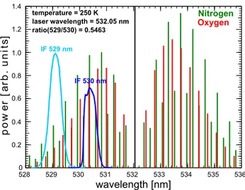
796 M. Alpers et al.: Temperature lidar measurements from 1 to 105 km wavelength [nm] 5280 529 530 531 532 533 534 535 536 0.2 0.4 0.6 0.8 1.0 1.2 1.4 p o w e r [a rb . u n it s ] Nitrogen Oxygen IF 529 nm IF 530 nm temperature = 250 K laser wavelength = 532.05 nm ratio(529/530) = 0.5463
Fig. 2. Power spectrum of the calculated Rotational Raman
spec-trum for the center wavelength of the IAP RMR laser transmit-ter (532.05 nm, black vertical line) and an example temperature of 250 K and measured transmission curves of the IF filters used for Rotation Raman measurements with the IAP RMR lidar. The power spectrum is normalized to the strongest N2Antistokes line, the filter
transmission curves are normalized to the peak value of the IF filter at 529 nm.
no mechanical chopper (see Fig. 1). To prevent PMT over-load, the backscatter signal is attenuated by about one order of magnitude. The transmission of the whole detector de-pending on wavelength has been measured with a high res-olution spectrometer in the relevant wavelength range. The measured filter transmission curves and the calculated Rota-tional Raman spectrum for an example temperature of 250 K is shown in Fig. 2. The quantum physical constants given by Butcher et al. (1971), Arshinov et al. (1983) and Vaughan et al. (1993) have been used to calculate the backscattered power of each single line by elemental, temperature depen-dent quantum physical laws. For both wavelength channels we have integrated the backscattered power at the various lines convoluted by the respective filter transmission. This procedure results in a function of temperature depending on the power ratio of the two wavelength channels for the spe-cific experimental configuration of the IAP RMR lidar. Ad-ditionally, we launch radiosondes for control on special occa-sions. At the lowest kilometers of the atmosphere the broad-ening of the Rayleigh line by Brillouin scatter might induce some additional, pressure-dependent signal in the rotational Raman channels. But it has been shown by Nedeljkovic et al. (1993) that with a sufficient narrow laser wavelength the contribution of the Rayleigh line can be neglected even at surface pressure. For the injection-seeded monomode laser of the IAP RMR lidar we can assume the Brillouin effect to be neglectable compared with the statistical error in the lowest bins. Presently, the detector contains only one PMT and a motorized IF filter wheel, which alternates between the
two Rotational Raman filters every 4000 laser pulses (about 2.2 min). This configuration does not require PMT sensi-tivity calibration, but allows temperature measurements only for temporal stable atmospheric transmission conditions. For example, passing low tropospheric clouds prevent Rotational Raman temperature measurements with this detector con-figuration because here atmospheric transmission becomes time-dependent. Therefore, the Rotational Raman detector of the IAP RMR lidar will be modified for simultaneous Ro-tational Raman operation in the future. With 1 h integration, temperature measurements up to 26 km are possible with a vertical resolution of 1 km and a temperature error of less than 10%. The Rotational Raman method works well down to about one kilometer altitude, where the backscatter sig-nals become too weak due to the geometric overlap function (bistatic system) and defocusing of the receiving telescope (limited depth of focus).
On its way through the atmosphere the emitted laser light is affected by various extinction processes: (1) Rayleigh scattering has a nearly homogeneous phase function, which reduces significantly the transmission in beam direction. The process is dependent on the number density of the air molecules and has a strong wavelength characteristic (∼λ−4). We use the Rayleigh scatter cross sections of Thome et al. (1999) and air molecule number densities calcu-lated from the corresponding zonal and monthly mean CIRA model profile (Fleming et al., 1990). By correcting the sig-nal for the Rayleigh extinction the calculated temperature decreases by about 1 K or less for altitudes of 20–30 km or above, respectively. (2) Ozone significantly absorbs light in the UV below about 350 nm (Huggins bands) and the visi-ble region between about 430 and 850 nm (Chappuis bands). For our ozone absorption correction we use the O3
absorp-tion cross secabsorp-tion from Bogumil et al. (2003) and mean ozone profiles from the “Berliner Ozon-Modell” (Fortuin and Langematz, 1994). The ozone correction amounts to about 3 K in the maximum altitude of the O3 layer. (3) Above
the troposphere and below about 35 km Mie scattering on stratospheric aerosols can significantly affect the backscatter signal. The number density within these aerosol layers is low enough to neglect extinction (except for periods after strong volcano eruptions as Mt. St. Helens or Pinatubo), but the en-hanced backscattering has to be considered. Unfortunately, neither the vertical number density profile nor the compo-sition of these stratospheric particles (i.e. their backscatter parameters) is known well enough for an exact backscatter ratio correction. For a rough compensation of the aerosol backscattering we introduce a mean aerosol layer with a backscatter ratio R of 1.06 below 28 km and decreasing to 1.00 above (<28 km: 1.06, 28–29 km: 1.05, 29–30 km: 1.04, 30–31 km: 1.03, 31–32 km: 1.02, >32 km: 1.00). These numbers are comparable (though more conservative) to the values of Fujiwara et al. (1982) and Zuev et al. (2001), who describe R numbers of up to 1.1 at 28–30 km altitude for volcanic-free conditions.
Temperature [K]
lidar signal [counts/1h*200m]
al
ti
tu
d
e
[k
m
]
100 110 120 140 0 10 20 30 40 50 60 70 80 90 0 1 2 3 4 5 6(a)
Rot. Raman 530 nm K-D Reson. 770 nm1 Rayl. 355 nm (high) Rayl. 532 nm (high) Rayl. 532 nm (low) Rot. Raman 529 nm RMR lidar: K lidar: 180 220 260 300(b)
K-D Reson. 770 nm1 Rayl. 355 nm (high) Rayl. 532 nm (high) Rayl. 532 nm (low) Rot. Raman RMR lidar: K lidar: CIRA86 (Feb. 23)Fig. 3. Example of a temperature lidar measurement with the IAP lidars at K¨uhlungsborn, Germany on 23 February 2003 at 00:30–01:30 UT.
Panel (a) shows the (background-corrected) raw lidar backscatter profiles of the different lidars and detectors. Panel (b) shows the temperature profiles, calculated from the raw data of panel (a). A smooth filter (0.6–3 km width, depending on altitude) and the corrections mentioned in the text have been applied.
The aerosol correction affects the temperatures by up to 8 K around 28 km. We are aware of the uncertainties of this procedure, but comparisons of the corrected Rayleigh tem-perature profiles with the Rotational Raman and radiosonde data show that the results are close to reality. Nevertheless, to avoid this uncertainty in the future, the IAP RMR lidar will be equipped with a vibrational Raman channel (which is not influenced by Mie backscattering) and/or a high Rotational Raman channel for the altitude region 15–40 km.
With the three methods described, complete temperature profiles between 1 and 105 km altitude can be obtained. The methods have identical time scales, observation geometries, vertical resolutions, and temperature errors (1 h integration time, about 0.5 mrad field of view (FOV), 1 km vertical res-olution, and less than 10% temperature error). This allows the determination of wave parameters from a large fraction of the planetary, tidal, or gravity wave scale.
Currently, the combined temperature measurements are limited to the nighttime. Daytime filtering for the individ-ual lidars is possible and already used for the IAP potassium resonance lidar (Fricke-Begemann et al., 2002). In general, the current solar background reduction techniques (FADOF, high resolution Fabry-Perot etalons, etc.) are not effective enough to allow calculations of vertically overlapping tem-perature profiles during daytime.
3 Measurements and results
Figure 3 shows an example of raw backscatter profiles, ob-tained by the IAP lidars (panel a), and temperature profiles (panel b), calculated from these data. The profiles of the different methods have altitude overlaps of a few kilometers with their neighbours. Additionally, the corresponding zonal and monthly mean CIRA model profile is plotted (Fleming et al., 1990). The main temperature error is produced by the signal statistics. The statistical temperature errors of the dif-ferent methods vary with altitude: The temperature profile of the potassium resonance lidar has small errors (less than 1 K) around the centre of the metal layer near 90 km and increas-ing errors at its bottom and top. Due to the exponential de-crease of the Rayleigh backscatter signals with altitude, the Rayleigh temperature errors are small at the bottom of the profiles (less than 1 K) and increase with altitude. The sit-uation is similar for the Rotational Raman temperature pro-file. Temperature values with more than 10 K uncertainty are discarded, leaving a reliable continuous temperature profile from 1 to 105 km.
Figure 3b includes the temperature profile calculated from the 355 nm (high) data (blue curve). Due to the lower sensi-tivity of the UV-branch the temperature profile is limited to an upper altitude of about 76 km. At an altitude of 42 km, the UV data is used for the exact determination of the dead
798 M. Alpers et al.: Temperature lidar measurements from 1 to 105 km
Temperature [K]
al
ti
tu
d
e
[k
m
]
200 220 240 260 280 300 0 5 10 15 20 25 30 35 40 Rayleigh 532 nm (low) Rot. Raman CIRA86 (Feb. 23) Radiosondes Feb. 22, 2003: Kühlungsborn, 2347-0139 UT Schleswig, 2200 UT Greifswald, 2200 UT RMR lidar:Fig. 4. Same period as Fig. 3b but limited to the altitude range 0–
40 km. In addition to the lidar data temperature profiles of three radiosondes are shown. One radiosonde was launched at 23:47 UT at K¨uhlungsborn (blue line) and two radiosondes were launched at about 22:00 UT at the DWD stations Schleswig and Greifswald (light blue and red lines).
time correction factor for the HSPMT. Due to the exponen-tial altitude dependence of the Rayleigh backscatter signal the temperature results at 532 nm are dependent on this pa-rameter only for the lowest 5 km range (<47 km). Above, for the HSPMT the dead time correction is much lower than 1%. Therefore, the good agreement between the 355 nm (high) and the 532 nm (high) results over the whole altitude range demonstrates the stability of the temperature calculation al-gorithm and the high data quality. In overlapping height ranges the temperatures retrieved from the different methods always agree within their error limits.
Figure 4 shows the vertical sub-range of Fig. 3b (low Rayleigh and Rotational Raman) below 40 km altitude to-gether with temperature data from a simultaneous radiosonde launched at K¨uhlungsborn and with data from two radioson-des launched at 22 h UT at the closest German Weather Service (DWD) stations at Schleswig and Greifswald (lo-cated about 100 km east and west of K¨uhlungsborn). Due to the limited ascent rate of a balloon-borne radiosonde (about 5 m/s) its profile in principle consists of data measured at dif-ferent times (data at the burst altitude was obtained about 2 h later than data obtained at the ground). Because we want to compare the Rayleigh lidar data with the radiosonde, in Figs. 3b and 4 we chose the lidar profile obtained during the second half of the radiosonde flight period, when the bal-loon was above 15 km. Below about 35 km the aerosol and
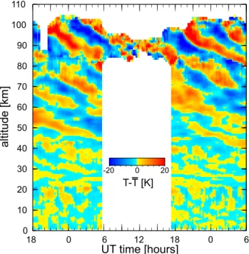
UT time [hours] 18 0 6 12 18 0 6 0 20 -20 T-T [K] 0 10 20 30 40 50 60 70 80 90 100 110 a lt it u d e [ k m ]
Fig. 5. Color-coded temperature deviation from the altitudinal mean for the time period between 22 February 2003, 18:00 UT and 24 February 2003, 06:00 UT, measured with the combined IAP li-dars. The profiles are calculated every 15 min with a 1-h running mean. The potassium resonance lidar detector is equipped with a narrow filter for daytime measurements, while Rayleigh and Rota-tional Raman temperature measurements are possible only during nighttime.
extinction corrected Rayleigh temperature profile fits well to the radiosonde data, indicating the importance of the various corrections. Radiosonde and rotational Raman lidar temper-ature profiles agree well within their experimental errors.
The measured temperature lidar profile of Fig. 3b shows a good agreement with the CIRA model values at troposphere and lower stratosphere altitudes, but large deviations at up-per stratospheric (about 20 K) and mesopause altitudes (up to 50 K!). These differences are caused by the different spatial and temporal basics of the two data sets: While the CIRA profile represents a monthly zonal mean with 10◦ latitude grid, the lidar profile is a local snapshot of the atmospheric temperature structure. The temperature profile of Fig. 3b shows clear wave structures with about 10–12 km vertical wavelength above 50 km altitude. At lower altitudes no clear wave structures are present. Short time processes such as wave structures and warming or cooling processes at hourly or daily scales strongly influence the local vertical structure of the temperature profile but are smoothed out in the zonal monthly mean profile of the CIRA model atmosphere.
The excellence of long-range and continuous night-time temperature lidar measurements becomes obvious with demonstrating the time dependence of the temperature pro-file and clearly illustrating vertical wave structures. Figure 5
shows the color-coded temperature deviation from the mean from 1 to 110 km altitude, measured with the IAP lidars at K¨uhlungsborn during 36 h on 22–24 February 2003. The de-viation is calculated as follows: For each altitude bin a tem-poral mean temperature was calculated from the observed profiles. This value was subtracted from the absolute perature values for each time step. At altitudes where tem-perature profiles overlap between two methods, the values with the lower temperature errors are used. Only tempera-ture values with less than 10 K error were considered. As explained above, Rayleigh and Rotational Raman measure-ments are limited to the nighttime while measuremeasure-ments with the potassium lidar are also possible in daylight. These dif-ferent observation periods of the potassium lidar and RMR lidar may result in phase shifts of the temperature variation. In order to avoid phase jumps around 80 km, the mean pro-file was calculated only for simultaneous sounding times, ac-cepting that this 12-h-mean may differ slightly from the daily mean in the potassium layer height.
The broad altitude range of these measurements allows si-multaneous observation of gravity wave excitation, filtering, and dissipation, although different waves may be observed at different points in the profile. Several wave parameters can be derived depending on altitude, e.g. amplitude, vertical wavelength, period, and potential energy. On 22–24 Febru-ary 2003 clear wave structures appear continuously above
40 km with downward propagating phase. The observed
phase velocity doubles from 50 km (−0.8 km/h) to 90 km (−1.7 km/h). From Fig. 5 a dominant vertical wavelength of 12–15 km can be derived, but superposed with longer and shorter waves especially in the upper stratosphere and lower mesosphere. Periods have been found between 9 and 14 h. Below about 20 km the variability is partly caused by noise. Due to the daytime operation capability of the potas-sium resonance lidar the wave structure at the 90 km altitude range is detected for the whole 36-h period. The high so-lar background signal decreases the usable altitude range of the potassium resonance lidar data to less than 10 km vertical width around 90 km altitude during daytime.
The data presented in Figs. 3, 4, and 5 was part of a 5-day continuous run from 22 to 27 February 2003. The complete data set will be analyzed in detail in a later publication in-cluding analytical wave parameter determination.
In this paper we have demonstrated using time resolved lidar backscatter data to retrieve continuous temperature pro-files from close to the ground up to about 105 km. While other methods for “quasi-continuous” temperature profiles combine different techniques and sounding methods, at the IAP we have assembled only lidar data obtained at the same location, but from different types of backscatter. The res-olution in time is 1 h or better in all altitudes, allowing for gravity and tidal wave studies. Currently, continuous tem-perature soundings are limited to the nighttime, although 24-h-measurements are desirable, e.g. for the examination of di-urnal and semididi-urnal tides. At present, daytime lidars cover
only the mesopause region down to about 85 km or the strato-sphere and lower mesostrato-sphere up to about 65 km. Future lidar technique developments are required to close this gap.
Acknowledgements. We thank T. K¨opnick from the IAP
K¨uhlungsborn for his assistance with the development and construction of our lidar instruments. Schleswig and Greifswald radiosonde data have been made available from the Met Office Global Radiosonde Data set through the British Atmospheric Data Center.
Edited by: G. Vaughan
References
Alpers, M., Eixmann, R., H¨offner, J., K¨opnick, T., Schneider, J., and von Zahn, U.: The Rayleigh-Mie-Raman lidar at IAP K¨uhlungsborn, J. Aerosol Sci., 30, Suppl. 1, 637–638, 1999. Arshinov, Yu. F., Bobrovnikov, S. M., Zuev, V. E., and Mitev, V. M.:
Atmospheric temperature measurements using a pure rotational Raman lidar, Appl. Opt., 22, 2984–2990, 1983.
Behrend, A. and Reichardt, J.: Atmospheric temperature profiling in the presence of clouds with a pure rotational Raman lidar by use of an interference-filter-based polychromator, Appl. Opt., 39, 1372–1378, 2000.
Bogumil, K., Orphal, J., Homann, T., Vogt, S., Spietz, P., Fleis-chmann, O. C., Vogel, A., Hartmann, M., Bovensmann, B., Fr-erick, J., and Burrows, J. P.: Measurements of molecular ab-sorption spectra with the SCIAMACHY pre-flight model: instru-ment characterization and reference data for atmospheric remote-sensing in the 230–2380 nm region, J. Photchem. Photbiol. A, 6271, 1–18, 2003.
Butcher, R. J., Willetts, D. V., and Jones, W. J.: On the use of a Fabry-Perot etalon for the determination of rotational constants of simple molecules – the pure rotational Raman spectra of oxy-gen and nitrooxy-gen, Proc. R. Soc. London Ser. A, 324, 231–245, 1971.
Dao, P. D., Farley, R., Tao, X., and Gardner, C. S.: Lidar ob-servations of the temperature profile between 25 and 103 km: evidence for strong tidal perturbation, Geophys. Res. Lett., 22, 2825–2828, 1995.
Fleming, E. L., Chandra, S., Barnett, J. J., and Corney, M.: Zonal mean temperature, pressure, zonal wind, and geopotential height as functions of latitude, Adv. Space Res., 10, 11–59, 1990. Fortuin, J. P. F. and Langematz, U.: An update on the global
ozone climatology and on concurrent ozone and temperature trends, SPIE, Atmospheric Sensing and Modeling, 2311, 207– 216, 1994.
Fricke, K. H. and von Zahn, U.: Mesopause temperatures derived from probing the hyperfine structure of the D2 resonance line of sodium by lidar, J. Atmos. Terr. Phys., 47, 499–512, 1985. Fricke-Begemann, C., Alpers, M., and H¨offner, J.: Daylight
rejec-tion with a new receiver for potassium resonance temperature lidars, Opt. Lett., 27, 1932–1934, 2002.
Fritts, D. C. and Alexander, M. J.: Gravity wave dynamics and effects in the middle atmosphere, Rev. Geophys., 41, 1, 1003, doi:10.129/2001RG000106, 2003.
Fujiwara, M., Shibata, T., and Hirono, M.: Lidar observation of sud-den increase of aerosols in the stratosphere caused by volcanic
800 M. Alpers et al.: Temperature lidar measurements from 1 to 105 km
injections – II. Sierra Negra event, J. Atm. Terr. Phys., 44, 811– 818, 1982.
Gross, M. R., McGee, T. J., Ferrare, R. A., Singh, U. N., and Kimvilakani, P.: Temperature measurements with a combined Rayleigh-Mie and Raman lidar, Appl. Opt., 36, 5987–5995, 1997.
Hauchecorne, A. and Chanin, M.-L.: Density and temperature pro-files obtained by lidar between 35 and 70 km, Geophys. Res. Lett., 7, 565–568, 1980.
Keckhut, P., Chanin, M.-L., and Hauchecorne, A.: Stratosphere temperature measurements using Raman lidar, Appl. Opt., 34, 5182–5186, 1990.
Nedeljkovic, D., Hauchecorne, A., and Chanin, M.-L.: Rotational Raman lidar to measure the atmospheric temperature from the ground to 30 km, IEEE Transactions on Geoscience and Remote Sensing, 31, 90–101, 1993.
Thome, K., Biggar, S., and Slater, P.: Algorithm Theoretical Basis Document for ASTER Level 2B1 – Surface radiance and ASTER Level 2B5 – Surface Reflectance, Remote Sensing Group of the Optical Sciences Center, University of Arizona, ATBD-AST-04, 45, http://eospso.gsfc.nasa.gov/eos homepage/for scientists/ atbd/docs/ASTER/atbd-ast-04.pdf, 1999.
Vaughan, G., Wareing, D. P., Pepler, S. J., Thomas, L., and Mitev, V. M.: Atmospheric temperature measurements made by rotational Raman scattering, Appl. Opt., 32, 2758–2764, 1993.
von Zahn, U. and H¨offner, J.: Mesopause temperature profiling by potassium lidar, Geophys. Res. Lett., 23, 141–144, 1996. Zuev, V. V., Burlakov, V. D., El’nikov, A. V., Ivanov, A. P.,
Chaikovskii, A. P., and Shcherbakov, V. N.: Processes of long-term relaxation of stratospheric aerosol layer in northern hemi-sphere after a powerful volcanic eruption, Atmos. Environ., 35, 5059–5066, 2001.