HAL Id: hal-00317243
https://hal.archives-ouvertes.fr/hal-00317243
Submitted on 1 Jan 2004
HAL is a multi-disciplinary open access
archive for the deposit and dissemination of
sci-entific research documents, whether they are
pub-lished or not. The documents may come from
teaching and research institutions in France or
abroad, or from public or private research centers.
L’archive ouverte pluridisciplinaire HAL, est
destinée au dépôt et à la diffusion de documents
scientifiques de niveau recherche, publiés ou non,
émanant des établissements d’enseignement et de
recherche français ou étrangers, des laboratoires
publics ou privés.
themagnetosphere during high speed streams
R. L. Kessel, I. R. Mann, S. F. Fung, D. K. Milling, N. O’Connell
To cite this version:
R. L. Kessel, I. R. Mann, S. F. Fung, D. K. Milling, N. O’Connell. Correlation of Pc5 wave power
inside and outside themagnetosphere during high speed streams. Annales Geophysicae, European
Geosciences Union, 2004, 22 (2), pp.629-641. �hal-00317243�
Annales
Geophysicae
Correlation of Pc5 wave power inside and outside the
magnetosphere during high speed streams
R. L. Kessel1, I. R. Mann2,3, S. F. Fung1, D. K. Milling2,3, and N. O’Connell1
1NASA Goddard Space Flight Center, Greenbelt, 20771 Maryland, USA 2Department of Physics, University of York, York, UK
3now at: Department of Physics, University of Alberta, Canada
Received: 17 March 2003 – Revised: 3 July 2003 – Accepted: 11 July 2003 – Published: 1 January 2004
Abstract. We show a clear correlation between the ULF wave power (Pc5 range) inside and outside the Earth’s mag-netosphere during high speed streams in 1995. We trace fluctuations beginning 200 RE upstream using Wind data, to fluctuations just upstream from Earth’s bow shock and in the magnetosheath using Geotail data and compare to pulsations on the ground at the Kilpisjarvi ground station. With our 5-month data set we draw the following conclusions. ULF fluctuations in the Pc5 range are found in high speed streams; they are non-Alfv´enic at the leading edge and Alfv´enic in the central region. Compressional and Alfv´enic fluctuations are modulated at the bow shock, some features of the waveforms are preserved in the magnetosheath, but overall turbulence and wave power is enhanced by about a factor of 10. Paral-lel (compressional) and perpendicular (transverse) power are at comparable levels in the solar wind and magnetosheath, both in the compression region and in the central region of high speed streams. Both the total parallel and perpendicu-lar Pc5 power in the soperpendicu-lar wind (and to a lesser extent in the magnetosheath) correlate well with the total Pc5 power of the ground-based H -component magnetic field. ULF fluc-tuations in the magnetosheath during high speed streams are common at frequencies from 1–4 mHz and can coincide with the cavity eigenfrequencies of 1.3, 1.9, 2.6, and 3.4 mHz, though other discrete frequencies are also often seen. Key words. Interplanetary physics (MHD waves and turbu-lence) – Magnetospheric physics (solar wind-magnetosphere interactions; MHD waves and instabilities)
1 Introduction
The possible role of Pc5 pulsations in energizing electrons to relativistic levels in the magnetosphere (e.g. Rostoker et al., 1998; Baker et al., 1998; Mathie and Mann, 2000) has increased the importance of understanding their excitation mechanisms. Pc5 pulsations, both in the equatorial outer Correspondence to: R. L. Kessel ([email protected])
magnetosphere (e.g. Kokubun et al., 1989; Anderson et al., 1991) and on the ground (e.g. Greenstadt et al., 1979; En-gebretson et al., 1991; Glassmier, 1995), have been linked to high speed solar wind streams in 1995. It is fairly well estab-lished that bow shock associated ULF fluctuations and pres-sure pulses can convect downstream, cause magnetosheath fluctuations and may be responsible for magnetospheric pul-sations, particularly in the Pc3-4 band (e.g. Greenstadt et al., 1983; Sibeck et al., 1989; Fairfield et al., 1990, Engebretson et al., 1991; Lin et al., 1991). However, gaps remain in under-standing the energy transfer process from high speed streams in the solar wind into the magnetosphere, particularly in the Pc5 frequency range. Below, we review the relevant knowl-edge of ULF waves and fluctuations (particularly Pc5 range) in high speed streams, in the magnetosheath and in the mag-netosphere. We also review theory and observations of trans-mission across the bow shock and magnetopause, and the current understanding of cavity and waveguide modes. 1.1 Waves and fluctuations in the solar wind
High speed solar wind streams occur during the declining phase of the solar cycle, originating from the Sun’s polar coronal holes. The polar coronal holes producing the fast so-lar wind reach their maximum latitudinal extent near sunspot minimum, confining the slow solar wind to a narrow equato-rial belt. Co-rotating Interaction Regions (CIRs) often occur at the leading edges of high speed streams as the high speed streams overtake the slower solar wind (Belcher and Davis, 1971; Tsurutani et al., 1995). Inward and outward propa-gating waves are found in these CIR regions and may be the result of turbulence driven by velocity shear (Coleman, 1968). The large-amplitude fluctuations found in the com-pression regions or colliding stream regions near the leading edge of streams cannot propagate away from these regions (Burlaga, 1970) and thus must persist within these regions for a considerable distance. In the central region of high speed streams, only outwardly propagating Alfv´en waves are found. Belcher and Davis (1971) suggested that these waves
may be generated in the solar atmosphere by turbulent pro-cesses. Theoretically, slow and fast MHD waves usually are quickly damped in collisionless plasmas with moderate to high plasma β (Barnes, 1966), leaving only outward propa-gating Alfv´en waves. These persist and can be quite pure in the inner solar system. Belcher and Davis showed the Alfv´en waves to be broad-band Pc5 range and below, with peaks at 1.67, 1.39, 1.11, 0.83, 0.37 mHz; though using Mariner 5 data they were limited to a Nyquist frequency of 1.67 mHz and could see nothing higher. Waves and fluctuations in high speed streams will impact the magnetosphere first at the bow shock.
1.1.1 Waves and fluctuations across boundaries
McKenzie and Westphal (1969, 1970) calculated amplitudes and directions of waves diverging from a fast hydromagnetic shock perturbed by a small amplitude hydromagnetic wave, using the Rankine-Hugoniot conservation equations across the shock, and Snell’s law. They found that fast magne-toacousic longitudinal waves are greatly amplified on pas-sage through the shock and that Alfv´enic waves are only moderately amplified. They suggested that this amplification might contribute to the turbulent nature of the Earth’s mag-netosheath and that fluctuations in the magmag-netosheath would tend to be predominantly longitudinal rather than Alfv´enic in nature. More recent MHD simulation studies indicate that Alfv´en/slow-mode waves and other discontinuities can be generated in the magnetosheath by the interaction between the bow shock and various MHD discontinuities or Alfv´en waves in the upstream solar wind (Lin et al., 1996). Obser-vationally, Sibeck et al. (1997), using simultaneous Wind and Geotail data, found clear evidence for Alfv´enic fluctuations propagating into the magnetosheath. The magnetosheath now is well known as a turbulent region, with most fluctu-ations originating in the solar wind or associated with the quasi-parallel bow shock (e.g. Crooker et al., 1981; Sibeck et al., 2000). Kwok and Lee (1984) calculated transmitted and reflected MHD waves at the magnetopause when it is a rotational discontinuity. They found that the reflected fast magnetosonic wave is significantly amplified and thus may contribute to magnetosheath turbulence.
Satellite observations have shown that the magnetopause can stably exist as either a tangential or rotational discon-tinuity (e.g. Russell and Elphic, 1978; Sonnerup et al., 1981). Under conditions when the magnetopause is a tan-gential discontinuity, Bn = 0, the magnetopause is closed and MHD wave transmission is not efficient (e.g. McKen-zie, 1970; Wolfe and Kaufmann, 1975). When the mag-netopause is a rotational discontinuity, Bn 6= 0, Kwok and Lee (1984) determined that MHD wave transmissions oc-curred over a wide range of incident angle and that the trans-mitted waves were usually amplified. They suggested that MHD wave transmission at an open magnetopause can be a significant mechanism for energy transport from the mag-netosheath to the magnetosphere. Furthermore, Kwok and Lee (1984) suggested that the valid range of wavelength,
λ, and wave frequency, f , for transmitted waves would be λ 1000 km (larger than the thickness of the magne-topause) and f 150 mHz based on vA = 150 km/s at the magnetopause. This designation favors ULF waves, par-ticularly Pc5 and lower frequency waves.
1.1.2 Waves in the magnetosphere
Dungey (1954) originally proposed that the regular periods of geomagnetic pulsations might be due to standing Alfv´en waves excited on geomagnetic field lines, later termed field line resonances (FLRs). When waves are observed in the magnetosphere, the peak amplitude occurs at the latitude that coincides with the field line that resonates at the wave fre-quency. Pc5 pulsations are common at latitudes between about 60◦ and 70◦(Hughes, 1994 and sources therein). In space these map from about the plasmapause to near the magnetopause on the dayside. Field line resonances are ob-served in the Pc5 range, with discrete frequencies at approx-imately 1.3, 1.9, 2.6, and 3.4 mHz (Ruohoneimi et al., 1991; Samson et al., 1992; Samson and Rankin, 1994). Samson et al. (1992) showed that these discrete frequencies were compatible with MHD waveguide and cavity modes in the magnetosphere. The Earth’s magnetospheric cavity extends from an outer boundary, possibly the magnetopause (or bow shock), to an internal turning point, possibly near the plasma-pause. In the cavity model energy is input into the magneto-sphere and the cavity as a whole rings at its own eigenfre-quenices, efficiently transporting energy at those frequencies to field lines in the magnetosphere and producing the classic field line resonance signature. The waveguide model is sim-ilar except that the cavity remains open downtail; waveguide modes propagate antisunward at the natural frequencies of the magnetosphere (e.g. Harrold and Samson, 1992; Mann et al., 1999).
It is commonly agreed that toroidal Pc5 pulsations are caused by an external source in the solar wind. The most frequently cited source of Pc5 pulsations in the magneto-sphere is the Kelvin-Helmholtz instability at the magne-topause (e.g. Dungey, 1955; Miura, 1992; Anderson, 1994; Engebretson et al., 1998). Mann et al. (1999) have recently shown that for very large flow speeds at the magnetopause flanks, the Kelvin-Helmholtz instability can energize body type waveguide modes. Other possible sources of Pc5 pul-sations have been proposed, such as upstream shock-related pressure oscillations that drive magnetopause surface waves with periods in the Pc5 range (Sibeck et al., 1989). Fair-field et al. (1990) suggested that upstream pressure varia-tions may be linked to magnetospheric compressions. En-gebretson et al. (1998 and sources therein) suggested that if the compression regions at the leading edges of high speed streams contain waves in the Pc5 range, they could provide a source of wave energy to the magnetosphere or that the waves could act as seed perturbations to drive boundary dis-placements that are amplified by the Kelvin-Helmholtz insta-bility. By contrast, Kepko et al. (2002) showed observations of pressure fluctuations at the same discrete frequencies in
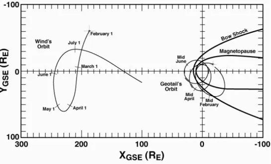
Fig. 1. Wind orbit from February through July 1995 and example Geotail orbits in mid February 1995, mid April 1995 and mid June 1995.
the solar wind as in the magnetosphere and suggested that the solar wind may be a direct source for discrete Pc5 pul-sations. Wright and Rickard (1995) showed that broad-band fluctuation power in the solar wind can lead to enhanced ex-citation of the magnetospheric cavity or waveguide modes, even if the spectral content of the upstream and magneto-sphere waves are different.
In this paper we investigate the linkage of waves and fluc-tuations in the solar wind, magnetosheath, and on the ground. We show a clear correlation between Pc5 wave power in-side and outin-side Earth’s magnetosphere during high speed streams in 1995. We trace the fluctuations beginning 200 RE upstream using Wind data, to fluctuations just upstream from the Earth’s bow shock and in the magnetosheath using Geo-tail data and compare to waves on the ground at the Kilpis-jarvi ground station. We show observations of waveforms, power spectral densities and total power in all regions and discuss probable transfer mechanisms.
2 Instruments and methods
For this study we use data from the Wind and Geotail satel-lites and from the Kilpisjarvi ground-based station. For the time period of this study, February through June 1995, Wind is located far upstream (∼ 200 RE) with yGSE varying be-tween ±60, as shown in Fig. 1. Geotail is orbiting the Earth, just transitioning to an orbit with an apogee of ∼ 30 RE. We show three orbits during the 5-month time frame in Fig. 1. The time interval of this study is dictated by the time when Geotail began its near-Earth orbit to when high speed streams became less regular.
We use data from the Magnetic Field Investigation (MFI) (Lepping et al., 1995) and the Solar Wind Experiment (SWE)
(Ogilvie et al., 1995) on Wind. We use magnetometer data from the Magnetic Field Measurement (MGF) (Kokubun et al., 1994) on Geotail. We use Kilpisjarvi (KIL) ground-based magnetometer data from the IMAGE magnetometer array (Luhr et al., 1998; www.geo.fmi.fi/image). KIL is located at 69.02◦geographic latitude, and is thus in a good position to measure Pc5 pulsations. For the space-based magnetome-ters we use 1-min resolution data to provide detail on the Pc5 portion of the spectrum (0–8.3 mHz) and 3-s resolution data to generate a broader ULF wave spectrum from 0–166 mHz. At Kilpisjarvi we have used 10-s resolution data (0–50 mHz) from the morning sector, summing only those 2-h bins which lie entirely within the range 05:00–11:00 LT.
For the satellite magnetometers we used the following analysis procedure. We first put the data into field-aligned coordinates and then calculated the power spectra separately for the parallel component and for the vector average of the perpendicular component. For the one-min data we used a sliding 128 point FFT (2 h) window and summed power in all the bands (1–8.3 mHz). For the 3-s data we used a sliding 512 point FFT (1/2 h) window and summed power in the 1– 10 mHz band. Each data set was detrended over the sliding point window (2 or 1/2 h) by subtracting an average value and then tapered using a Parzen window. The data were processed using a fast Fourier transform algorithm to cre-ate power spectral densities (PSD) and then the PSDs were summed to obtain total power. The window was advanced for each data point to create a running spectrum and in addi-tion, an average value was determined for every 6- and 24-h worth of data.
For the ground-based magnetometer we used a sliding 720 point FFT window to the H component, advanced by succes-sive half hour intervals through the day. A daily Pc5 power value was calculated by summing power in the 1–10 mHz
107 106 105 104 103 102 105 104 103 102 106 105 104 103 102 Pc5 Power Pc5 Power Pc5 Power
1 Feb 95 1 Mar 95 1 Apr 95 Wind
Geotail Magnetosheath Geotail Solar Wind
Wind KIL
KIL (x 0.1)
1 May 95
Wind and Geotail Parallel Pc5 Power
1 Jun 95 1 Jul 95 +
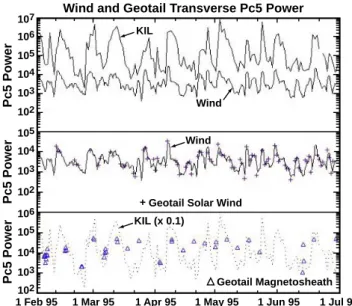
Fig. 2. Top panel: Pc5 pulsation power at Kilpisjarvi
ground-based station (upper curve) compared to parallel Pc5 power at Wind (lower curve). Middle panel: parallel Pc5 power at Wind (curve) and Geotail (crosses) with both in the solar wind. Bottom panel: Pc5 pulsation power at Kilpisjarvi (dotted curve) and parallel Pc5 power at Geotail in the magnetosheath (triangles).
band from an average of the windows centered in the local time morning sector. These data are nearly identical to those published in Mathie and Mann (2000), except that in the lat-ter all bins in the morning sector were summed, not averaged.
3 Observations
Figure 2 compares Pc5 wave power inside and outside of the magnetosphere during 5 months in 1995. The peaks in power coincide with the peaks in solar wind speed in the high speed streams, as shown previously by Mathie and Mann (2000). The top panel of Fig. 2 shows ULF wave power in the Pc5 range from the H component at Kilpisjarvi (upper curve) and the parallel component of Pc5 power from Wind (lower curve). These two curves represent the extreme locations ex-amined in this study, i.e. far upstream and on the ground. The correlation between these two curves is good, as can be seen by eye; the correlation coefficient is 0.61. The middle panel shows the same parallel Pc5 power from Wind to guide the eye along with the sparse points of parallel Pc5 power from Geotail in the solar wind (crosses). The Geotail data in the solar wind are not continuous because Geotail’s or-bit also takes it into the magnetosheath and magnetosphere. These two sets of data in the middle panel are nearly coin-cident, but in some cases, the power at Geotail is slightly higher. In these cases Geotail is connected to a quasi-parallel bow shock for an extended time and the Pc5 power is en-hanced. The bottom panel shows the Pc5 wave power from Geotail in the dusk magnetosheath (triangles), along with the H-component Pc5 power from KIL shifted down by an order
107 106 105 104 103 102 105 104 103 102 106 105 104 103 102 Pc5 Power Pc5 Power Pc5 Power
1 Feb 95 1 Mar 95 1 Apr 95 1 May 95 1 Jun 95 1 Jul 95
Wind and Geotail Transverse Pc5 Power
Geotail Solar Wind + Geotail Magnetosheath Wind KIL Wind KIL (x 0.1)
Fig. 3. Top panel: Pc5 pulsation power at Kilpisjarvi ground-based
station (upper curve) compared to perpendicular Pc5 power at Wind (lower curve). Middle panel: perpendicular Pc5 power at Wind (curve) and Geotail (crosses) with both in the solar wind. Bottom panel: Pc5 pulsation power at Kilpisjarvi (dotted curve) and per-pendicular Pc5 power at Geotail in the magnetosheath (triangles).
of magnitude. The magnitude of the dusk magnetosheath Pc5 power lies between the solar wind and ground-based levels but follows a similar pattern, though the sparse points make the correlation difficult to see without the downshift in the KIL power curve to guide the eye. There were only 3 dawn-side magnetosheath points and each occurred indawn-side a com-pression region, so it was not possible to establish any trend or see any correlation between the dawnside magnetosheath and KIL.
Figure 3 is similar to Fig. 2, but now we compare the H component at KIL with perpendicular power at Geotail and Wind. In comparing Fig. 2 and Fig. 3 we see that the parallel (compressional) power is at approximately the same level as the perpendicular (transverse) power in both the so-lar wind and magnetosheath. The correlation between the H component Pc5 power at Kilpisjarvi and perpendicular Pc5 power at Wind is also good, with a correlation coefficient of 0.58. The middle panel of Fig. 3 shows that the perpendicu-lar power at Wind and Geotail in the soperpendicu-lar wind correlates as well as it did in the parallel case. There are again cases when Geotail power is higher due to being connected to a quasi-parallel bow shock. This is more often true starting in April, when Geotail’s orbit swings around to spend more time on the dawn side. The bottom panel of Fig. 3 is similar to the bottom panel of Fig. 2, i.e. transverse Pc5 wave power from Geotail in the dusk magnetosheath (triangles) along with H -component Pc5 power from KIL shifted down by an order of magnitude. The correlation here is as good as it was in the parallel case.
800 600 500 700 400 300 100 80 60 40 20 30 20 10 10 8 6 4 2 0 P (nPa) B (nT) Cone Angle Vsw (km/s) 6 8 10 12 Day of April 1, 1995 MS SW SW Geotail Wind 14 16 18 20
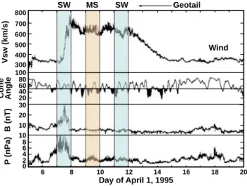
Fig. 4. Classic high speed stream, 5–20 April 1995. From top to
bottom: solar wind high speed stream, cone angle, magnetic field magnitude, ram pressure.
We look in detail at one classic high speed stream during the five month interval in 1995, 5–20 April. The top panel of Fig. 4 shows that the solar wind speed has an initial steep increase, with the speed remaining high for 4 days before gradually trailing off. At the leading edge of the stream there is a compression region, as seen by the increases in dynamic pressure and magnetic field magnitude. This compression re-gions occurs nearly a day before the increase in speed. This is typical of other streams in this study and agrees with the re-sults of Engebretson et al. (1998), who showed that the peak pulsation power at two ground stations typically occurred about 1 day before the peak solar wind velocity. The high speed streams in 1995 follow this general pattern, but not all are as steep or as long lasting, and some have more than one compression region.
The second panel shows the IMF cone angle, the angle between the x-GSE axis and the magnetic field. During the high speed stream, the cone angle is less than 50◦more than half the time, whereas outside the stream the cone angle is greater than 50◦. This is also typical of high speed streams during this interval. During this high speed stream in April, Geotail’s orbit passed through the solar wind at the leading edge and then through the magnetosheath and solar wind in the central region (sub-intervals marked in Fig. 4). The type of waves seen are characteristic of each region of the high speed stream, and differ in the solar wind, magnetosheath, and on the ground, as we show in the following examples. Ideally, we would look at examples when Wind, Geotail, and KIL are all on the dawn side. However, with this data set we are limited to two of the three at any one time.
3.1 Leading edge of high speed stream
At the leading edge we show three examples. The first is a comparison of Wind and Geotail data (7 April 1995),
Wind Satellite - 7 April 1995
30 20 10 -200 -300 -300 -400 -400 Vtrans (z) Vtrans (1) Vpar (km/a) Np Btrans (z) Btrans (1) Bpar Bmag (nT) -500 -500 -600 0 -50 -100 -150 -200 30 30 20 20 -20 16:00 14:00 18:00 20:00 22:00 10 -10 10 15 10 -10 -15 -10 0 0 0 20 25 15 10 5 5 -5
Fig. 5. Wind data in the solar wind inside the compression region,
7 April 1995. Top panel: magnetic field and density; second panel:
b||and v||, bottom two panels: transverse components of b and v.
when both are in the solar wind on the dusk side, with Wind ∼ 200 RE upstream and Geotail just in front of the bow shock. Then we compare Wind and Geotail data, when both are on the dawn side (13:00–20:00 UT, 19 June 1995), Wind is still ∼ 200 REupstream but Geotail is in the magne-tosheath. We have no intervals when Geotail is in the dawn magnetosheath with KIL also on the dawn side. We show instead a comparison of Wind and KIL data when both are on the dawn side (02:00–10:00 UT 19 June 1995).
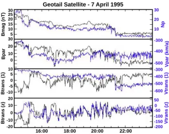
Our first interval corresponds to the first sub-interval in Fig. 4, when both Wind and Geotail are in the solar wind on the dusk side. We show perturbations in magnetic field and velocity in field-aligned coordinates during the compression region on 7 April 1995: one parallel and two transverse com-ponents in the bottom three panels of Fig. 5. In the top panel we show magnetic field magnitude and ion density. Both of these are high at the beginning of the plot, decrease just before 14:00 UT and again at about 20:30 UT. Because the magnetic field magnitude and the density are changing sig-nificantly up until 20:30 UT, we expect the fluctuations not to be Alfv´enic in this region. Aperiodic Alfv´en waves would show a correlated variation between the components, as de-fined by the relation, b = ±(4πρ)1/2v (Belcher and Davis, 1971). This is not the case, as can be seen in the bottom 3 panels of Fig. 5. After the drop in magnetic field magnitude and ion density at about 20:30 UT the values remain fairly steady for the remainder of the plot.
Figure 6 follows the same format as Fig. 5 but has data from Geotail in the solar wind. There are many similarities between Figs. 5 and 6. The top panel shows magnetic field magnitude and density drops about 45 min earlier in Fig. 5 compared to Fig. 6 which is expected because of the differ-ence in location. If the fluctuations are trapped in the com-pression region and the comcom-pression region encompasses a large area we might expect to see similar fluctuations at Wind
Geotail Satellite - 7 April 1995 30 20 10 -300 -300 -400 -400 Vtrans (z) Vtrans (1) Vpar (km/a) Np Btrans (z) Btrans (1) Bpar Bmag (nT) -500 -500 -600 50 0 -50 -100 -150 -200 30 30 20 20 -20 16:00 18:00 20:00 22:00 10 10 10 -10 -10 0 0 0 20 25 15 10 5 5 -5
Fig. 6. Geotail data in the solar wind inside the compression region,
7 April 1995. Top panel: magnetic field and density; second panel:
b||and v||, bottom two panels: transverse components of b and v.
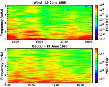
Wind - 7 April 1995 Geotail - 7 April 1995 14:00 16:00 18:00 20:00 22:00 14:00 16:00 18:00 20:00 22:00 00:00 8 6 4 2 Frequency (mHz) PSD B Par 0 8 6 4 2 Frequency (mHz) 0 104 103 102 101 100 10-1 10-2 10-3 PSD BPar 104 103 102 101 100 10-1 10-2 10-3
Fig. 7. PSD for Wind (top panel) and Geotail (bottom panel) on 7
April 1995.
and at Geotail even with almost 200 RE separation between them in x and 20–30 RE separation in y. There are similar-ities between the fluctuations but they are not identical. The level of fluctuations of the components are similar and it is possible to pick out some similar peaks and dips in the com-ponents. For example in the second panels there are similar dips in Bparat ∼16:00 UT in Fig. 5 and ∼17:00 UT in Fig. 6. Additionally, the vt ranscomponent in the third panels begins low and the trend is to increase slightly in magnitude and then become steady with a sharp increase in magnitude coin-ciding with a drop in B magnitude and density ∼20:30 UT in Fig. 5 and ∼21:20 UT in Fig. 6. Although they do not match up in all details there is enough similarity to believe that they are portions of one extended region.
Wind Satellite - 19 June 1995
20 10 15 5 800 500 600 400 200 400 Vtrans (z) Vtrans (1) Vpar (km/a) Np Btrans (z) Btrans (1) Bpar Bmag (nT) 300 200 100 100 50 0 -50 -100 -150 20 20 -20 13:00 14:00 15:00 16:00 17:00 18:00 19:00 10 -5 15 5 20 -5 -10 10 -5 0 5 5 0 15 10 15 5 10 0
Fig. 8. Wind data in the solar wind inside the compression region,
19 June 1995. Top panel: magnetic field and density; bottom three panels: field-aligned and perpendicular components of b and v.
Power Spectral Densities (PSDs) in the Pc5 range associ-ated with the parallel (compressional) component are shown for Wind (top panel) and Geotail (bottom panel) on 7 April 1995 in Fig. 7. Both satellites are in the solar wind and the color scales are identical for both panels in this figure. The two panels are not identical, but like the waveforms there are many similaries. In both panels there are three large PSD enhancements extending over much of the Pc5 range. At Wind these enhancements are centered at about 13:00 UT, 16:00 UT, and 20:00 UT, while at Geotail they occur approx-imately an hour later in each case. The peak power is primar-ily in the 0–4 mHz range, though at Geotail there are a few peaks up to 6 mHz. The discrete power peaks are not identi-cal at the two satellites, but they are similar. For example, the enhancement centered at 16:00 UT at Wind and 17:00 UT at Geotail has broad band power under 1.7 mHz in each case with discrete peaks at 2.3, 3.0, and 3.8 mHz for Wind and 2.5, 2.9, 4.0 and 4.6 mHz for Geotail.
We chose another interval in which both Wind and Geotail were on the dawn side with Wind still ∼ 200 RE upstream but with Geotail in the magnetosheath. Figures 8 and 9 again show b and v fluctuations in field-aligned coordinates, as in Figs. 5 and 6. Figure 8 shows the magnetic field and plasma fluctuations at Wind. There is a drop in magnetic field mag-nitude and density at ∼13:40 UT, shown in the top panel, fol-lowed by some smaller fluctuations in each. After 13:40 UT the pressure also decreases (not shown) but is still higher than that typically found in the central region. Before 13:40 UT Wind is clearly in the compression region and the fluctua-tions are non-Alfv´enic, as can be seen in the bottom three panels of Fig. 8. After 13:40 UT the nature of the waves changes; they exhibit some anticorrelation between the mag-netic field and velocity components that could be an indica-tion of shear Alfv´en waves or fluctuaindica-tions (Kivelson and Rus-sell, 1995) and a transition to the central region of the stream.
Geotail Satellite - 19 June 1995 30 20 10 0.5 6 0.0 -0.5 -1.0 -1.5 4 Vtrans (z) Vtrans (1) Vpar (km/a) Np Btrans (z) Btrans (1) Bpar Bmag (nT) 2 0 2.0 1.5 1.0 0.5 0.0 80 3 4 2 40 -60 14:00 15:00 16:00 17:00 18:00 19:00 1 -1 20 20 -60 -20 -40 -20 0 0 0 60 40 20 10 -10
Fig. 9. Geotail data in the magnetosheath inside the compression
region, 19 June 1995. Top panel: magnetic field and density; bot-tom three panels: field-aligned and perpendicular components of
b and v.
However, the fluctuations in the magnetic field and velocity components are somewhat irregular during the intervals after 13:40 UT, when fluctuations in density and magnetic field magnitude increase, e.g. between 15:45 UT and 17:15 UT. The magnetosheath fluctuations for magnetic field and veloc-ity at Geotail (Fig. 9) are enhanced over those seen at Wind, especially in the compression region up to about 15:00 UT. The fluctuations in density remain high throughout the inter-val and the amplitude is especially high during the interinter-val 16:30 UT to 18:20 UT. The anticorrelations are not evident at Geotail. We previously showed larger ULF wave fluctu-ations in the magnetosheath in Figs. 2 and 3, so this result is not surprising. We calculated a time lag between the two satellites based on x separation and a solar wind speed of about 40 min. Starting at about 14:05 UT in Fig. 8 and at about 14:40 UT in Fig. 9, we can pick out a similar feature in the B-parallel component, a multiple dip, at both Wind and Geotail. There are other similarities, but there are more dif-ferences, most likely due to modulation at the bow shock or reflection at the magnetopause.
Figure 10 shows the power spectral density (PSD) asso-ciated with the parallel (compressional) component at Wind (top panel) and Geotail (bottom panel). The color scales are different in each panel, in order to pull out the peaks in the spectrum. The total power increases as we move from the top panel to the bottom panel. We first compare general trends in the solar wind (top panel) with general trends in the mag-netosheath (bottom panel). There are five intervals of PSD increase at Wind (top panel): at the begining of the inter-val until about 13:15 UT; from about 13:45 UT until about 15:15 UT; centered at about 16:15 UT, from about 17:15 UT until about 18:15 UT; and and centered at about 19:00 UT. These intervals are not exactly mirrored at Geotail (bottom panel) but there are some similarities. At Geotail we could
Wind - 19 June 1995 Geotail - 19 June 1995 13:00 15:00 17:00 19:00 13:00 15:00 17:00 19:00 8 6 4 2 Frequency (mHz) PSD B Par 0 8 6 4 2 Frequency (mHz) 0 104 103 102 101 100 10-1 10-2 10-3 PSD B Par 103 102 100 10-2
Fig. 10. PSD for Wind (top panel) and Geotail (bottom panel) on
19 June 1995.
define two intervals of PSD increase, starting at 13:00 UT until about 16:00 UT, that could be related to the first two intervals at Wind, though in the magnetosheath the intervals have nearly merged and have similar frequency peaks below 4 mHz. The third interval at Geotail has peaks throughout the Pc5 frequency range in contrast to the third interval at Wind which has power only below 2 mHz. The fourth interval at Wind has no clear corresponding power at Geotail, and the fifth interval is small, both at Wind and Geotail.
Throughout the region there are peaks in Pc5 wave power that fall primarily between 1 and 5 mHz in the solar wind (Fig. 10 top panel) and between 1 and 7 mHz in the mag-netosheath (bottom panel). We can compare the power associated with the waveform features starting at Wind at 14:05 UT and at Geotail at 14:40 UT (Figs. 8 and 9). We see some similar peaks in the PSD at these times in Fig. 10. Wind (top panel) has 2 dominant broad-band peaks cen-tered 0.9–1.2 mHz and 1.7–2.2 mHz, and other minor peaks at 2.6 mHz, 3.4 mHz, 5 mHz, and 7 mHz. Geotail (bottom panel) has a broad-band peak near 1mHz, and other peaks at 2.4, 3.0 and 3.6, 5, and 6 mHz. The frequencies associated with the other intervals do not compare as well between the solar wind and magnetosheath. In summary, there are some similar general trends in PSD in the solar wind and magne-tosheath at the leading edge of high speed streams, and, as noted above, there is an interval in this example where there are peaks in PSD at the same frequency for Wind and Geo-tail. But there are also cases where there is power in the solar wind with little power in the magnetosheath and vice versa.
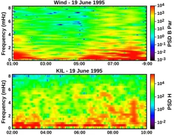
The third interval is earlier in the day on 19 June 1995 and is a comparison between Wind ∼ 200 RE upstream and KIL, ground-based station. There are no similarities between the waveforms at Wind and KIL which is not suprising since Wind measures the solar wind magnetic field while KIL mea-sures the Earth’s instrinsic field, as well as influences from magnetospheric and ionospheric currents. We show them for
Wind Satellite - 19 June 1995 100 80 60 40 20 -40 -340 -60 -80 -100 -120 -360 Vtrans (z) Vtrans (1) Vpar (km/a) Np Btrans (z) Btrans (1) Bpar Bmag (nT) -380 -400 60 40 20 0 -20 -40 -60 25 20 -20 02:00 04:00 06:00 08:00 10 -10 -20 10 10 20 -10 -10 0 0 0 20 15 10 5 5 -5
Fig. 11. Wind data in the solar wind inside the compression region,
19 June 1995. Top panel: magnetic field and density; bottom three panels: field-aligned and perpendicular components of b and v.
150 100 50 400 300 200 100 150 100 50 02:00 04:00 06:00 08:00 10:00 0 D (nT) H (nT) Bmag (nT)
KIL Ground Based Station - 19 June 1995
Fig. 12. KIL ground-based data during the time when the
com-pression region of a high speed stream impacts the Earth’s magne-tosphere on 19 June 1995. Top panel: magnetic field magnitude; middle panel: H component; bottom panel: D component.
reference in Figs. 11 and 12. Figure 11 follows the same for-mat as previous waveform plots shown here, that is, the mag-nitude of the magnetic field and density in the top panel, and the field-aligned and perpendicular components of magnetic field and velocity fluctuations in the bottom three panels. The fluctuations at Wind are again non-Alfv´enic, as we have seen consistently for the leading edge of high speed streams. We show the ground-based magnetometer data at KIL (Fig. 12) as variometer data, that is, as a range rather than absolute values. We show the magnitude and H and D components in top to bottom panels, and do not have velocity or den-sity data. There is no correlation between the Wind and KIL large-scale waveforms, so we next look at the associated ultra low frequency wave power (Pc5 range).
Wind - 19 June 1995 KIL - 19 June 1995 01:00 03:00 05:00 07:00 -9:00 02:00 04:00 06:00 08:00 10:00 8 6 4 2 Frequency (mHz) PSD B Par 0 8 6 4 2 Frequency (mHz) 0 104 104 103 102 102 101 100 100 10-1 10-2 10-2 10-3 PSD H
Fig. 13. PSD for Wind (top panel) and KIL (bottom panel) on 19
June 1995.
Figure 13 shows the power spectral density (PSD) associ-ated with the parallel (compressional) component at Wind (top panel) and the H component at KIL (bottom panel). These are the same components as were used in Fig. 2 (top panel). The color scales are different in each panel in Fig. 13, in order to pull out the peaks in the spectrum. The KIL power bands are somewhat wider than those at Wind due to the resolution of the data. There are general trends in the two panels that are similar: an enhancement in power be-tween 0 and 4 mHz at the beginning of the plot; a depletion in PSD between 03:00 UT and 05:00 UT (top) and between 04:00 UT and 06:00 UT (bottom); and increased PSD be-tween 06:00 UT and 09:00 UT (top) and bebe-tween 07:00 UT and 10:00 UT (bottom). The peaks in PSD occur in the fre-quency range of 0–4 mHz for Wind, but extend to a higher frequency for KIL ∼06:00 UT, ∼07:30 UT, and ∼09:15 UT. Although there is similarity in the general trends, there is no one-to-one match up between individual frequency peaks at Wind with those at KIL. For example, at ∼09:15 UT at KIL there is broad-band power from 1–5 mHz, while at Wind at ∼08:15 UT the highest power (also broad-band) is from 0– 1.5 mHz with a lower broad-band power from 1.6 to 2.1 mHz, and more discrete peaks at 2.6–2.7, 3.4, and 3.6 mHz. It is in-teresting that the cavity eigenfrequencies of 1.3, 1.9, 2.6, and 3.4 are all evident in the solar wind data during the largest broad-band increase at KIL ∼09:15 UT.
3.2 Central region of high speed stream
In the central region we show two examples. First, we show a comparison of Wind and Geotail data (9 April 1995) when both are on the dusk side, with Wind ∼ 200 RE upstream and Geotail in the magnetosheath. There are no intervals in the central regions of high speed streams with Geotail on the dawn side, but we show a comparison of Wind and KIL data when both are on the dawn side (2 March 1995).
Wind Satellite - 9 April 1995 5 4 3 2 1 -500 -150 -550 -600 -650 -200 Vtrans (z) Vtrans (1) Vpar (km/a) Np Btrans (z) Btrans (1) Bpar Bmag (nT) -250 -300 40 50 0 -20 -40 -60 -80 8 8 -6 01:00 02:00 03:00 04:00 05:00 06:00 07:00 4 6 2 6 -2 -4 -4 4 -2 0 2 2 0 6 4 6 2 4 0
Fig. 14. Wind data in the solar wind in the central region of the
high speed stream on 9 April 1995. Top panel: magnetic field and density; bottom three panels: field-aligned and perpendicular com-ponents of b and v.
Geotail Satellite - 9 April 1995
15 10 5 -400 -50 -450 -500 -550 -100 Vtrans (z) Vtrans (1) Vpar (km/a) Np Btrans (z) Btrans (1) Bpar Bmag (nT) -150 -200 200 150 100 50 0 25 20 -20 02:00 03:00 04:00 05:00 06:00 07:00 08:00 10 -10 15 10 20 -5 -10 0 5 0 20 15 10 5 10 0
Fig. 15. Geotail magnetosheath data in the central region of the
high speed stream on 9 April 1995. Top panel: magnetic field and density; bottom three panels: field-aligned and perpendicular com-ponents of b and v.
For the first example both Wind and Geotail are on the dusk side in Figs. 14 and 15, respectively. This is the second sub-interval shown in Fig. 4 and it occurs on 9 April 1995. Figures 14 and 15 follow the same format as previous wave-form plots shown here, that is, the magnitude of the mag-netic field and density in the top panel and the field-aligned and perpendicular components of magnetic field and velocity fluctuations in the bottom three panels. In Fig. 14, the bot-tom three panels show the Alfv´enic nature of the fluctuations at the Wind satellite in the solar wind. The magnetic field magnitude and density in the top panel are not as highly vari-able as they were in the compression region, although there is some evidence of a compressional wave in the magnetic
Wind - 9 April 1995 Geotail - 9 April 1995 00:00 02:00 03:00 06:00 01:00 03:00 05:00 07:00 8 6 4 2 Frequency (mHz) PSD B Par 0 8 6 4 2 Frequency (mHz) 0 104 103 102 101 100 10-1 10-2 10-3 PSD B Par 104 102 100 10-2
Fig. 16. PSD for Wind (top panel) and Geotail (bottom panel) on 9
April 1995.
field magnitude. Each of the components of magnetic field and velocity are correlated (bottom three panels of Fig. 14) but the correlation is not perfect.
In the magnetosheath in Fig. 15 the amplitude of the fluc-tuations is increased and the flucfluc-tuations are less Alfv´enic. Based on timing considerations these fluctuations should be from the same region of the high speed stream. It is also possible to spot some similarities such as the higher level of Bparat the beginning of each plot (second panels), followed by a drop at about 03:00 UT in Fig. 14 and at about 03:45 UT in Fig. 15. The absolute value of each component is higher in the magnetosheath than in the solar wind but this is expected after crossing the bow shock. The Alfv´en fluctuations in the central region of high speed streams appear to retain more of their original character after crossing the bow shock than do the compressional fluctuations at the leading edge.
Figure 16 shows the power spectral density associated with the parallel (compressional) component at Wind (top panel) and Geotail (bottom panel) on 9 April 1995. The color scales are different in each panel, in order to pull out the peaks in the spectrum. The total power increases as we move from the top panel to the bottom panel. The power at both Wind and Geotail is lower than in Fig. 7, but this is due to being in the central region of the high speed stream. There is a power enhancement centered at about 04:00 UT at Geotail that may be related to the enhancement at Wind centered at about 03:00 UT, taking into account timing differences be-tween the satellite locations. The individual power peaks within this enhancement are similar but not identical for the two satellites. Peaks at Wind (top panel) are evident at 1.0, 1.5, and 1.9 mHz. Geotail power (bottom panel) is broad-band below 1.5 mHz with another broad-broad-band increase cen-tered near 1.8 mHz and narrower peaks at 2.8 and 3.6 mHz. After this enhancement, there is a power reduction at Wind but at Geotail there is another power enhancement similar to the first one. Then we can see the edge of enhancements at
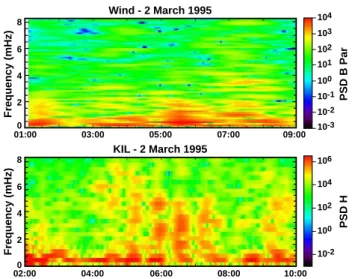
Wind - 2 March 1995 KIL - 2 March 1995 01:00 03:00 05:00 07:00 09:00 02:00 04:00 06:00 08:00 10:00 8 6 4 2 Frequency (mHz) PSD B Par 0 8 6 4 2 Frequency (mHz) 0 104 103 102 101 100 10-1 10-2 10-3 PSD H 106 104 102 100 10-2
Fig. 17. PSD for Wind (top panel) and KIL (bottom panel) on 2
March 1995.
Wind and Geotail that again, due to timing considerations, may be related.
For the second example both Wind and KIL are making observations on the dawn side, with Wind 200 REupstream (y = −5 RE). We do not show the waveforms for this exam-ple because there is no similarity between them. The fluctu-ations at Wind are Alfv´enic, which is expected in the central region of a high speed stream. We are interested in com-paring the Pc5 frequency range at Wind and KIL. Figure 17 shows the power spectral density associated with the parallel (compressional) component at Wind (top panel) and the H component at KIL (bottom panel) on 2 March 1995. There are four enhanced intervals at Wind: between 01:00 UT and 02:00 UT; centered at about 03:30 UT; between 05:00 UT and 06:00 UT; and centered at about 07:30 UT. There is an enhanced interval between 02:00 UT and 03:00 UT at KIL that may be related to the first interval at Wind, in each case the power is enhanced at frequencies less than about 2 mHz and is fairly broad-band. However, between 04:00 UT and 08:00 UT the KIL PSD (bottom panel) bares little resemblance to the Wind PSD (top panel). Both in-tervals are enhanced over ambient levels, but the nature of the enhancements are quite different. At Wind, the enhance-ments occur for frequencies less than about 2 mHz, except for the enhancement centered at about 07:30 UT, in which case the power is enhanced up to about 4 mHz. However, at the corresponding time at KIL, there is a power reduction. The KIL PSD plot (bottom panel) shows four distinct in-tervals of about 30 min each with broad-band enhancements stretching up to about 6 mHz. We again note that the cavity eigenfrequencies of 1.3 and 1.9 are both evident in the solar wind data during the largest broad-band increase at KIL at about 06:30 UT. With the possible exception of the interval at 06:30, it would seem that between 04:00 UT and 08:00 UT the power enhancements at Wind and KIL are not directly re-lated.
4 Discussion and conclusions
A fundamental question that remains unanswered is “what drives Pc5 power in the magnetosphere?” There are two fa-vorite hypotheses: (1) that fluctuations in the solar wind di-rectly drive ULF power in the magnetosphere (e.g. Kepko et al., 2002) or that broad-band fluctuation power in the so-lar wind can lead to enhanced excitation of the magneto-spheric cavity or waveguide modes, even if the spectral con-tent of the upstream and magnetosphere are different (e.g. Wright and Rickard 1995); or (2) that the fast solar wind streams lead to an enhanced Kelvin-Helmholtz instability on the flanks, particularly the dawn flank, and that this leads to enhanced Pc5 power inside the magnetosphere through the surface mode hypothesis (e.g. Dungey, 1955; Miura, 1992; Anderson, 1994), or by the energisation of body waveguide modes (e.g. Mann et al., 1999). We focus our discussion on fluctuations and wave transmission to investigate (1) above. We can inquire if ULF fluctuations themselves, particularly in the Pc5 range, are found in high speed solar wind streams. If so, are they modulated crossing the bow shock? How do the magnetosheath fluctuations compare with the solar wind fluctuations? How do the solar wind or magnetosheath fluc-tuations interact with the magnetopause and magnetosphere? In answering these questions we can reach a deeper under-standing of how energy is transmitted from the solar wind to the magnetosphere and what drives Pc5 power.
ULF fluctuations in the Pc5 range are found in high speed streams. All of the solar wind examples shown here, both at the leading edge and in the central region of high speed streams, exhibit fluctuations in the Pc5 range. These exam-ples are representative of the 5-month data set and the dis-cussion relates to all. The Pc5 frequency range dominates over higher frequency ULF fluctuations, with the power be-ing several orders of magnitude greater than the Pc3 or Pc4 power inside high speed streams (not shown). Lower fre-quency fluctuations (under 1 mHz) have higher or compara-ble power to the Pc5 range, but these fluctuations may be less geo-effective than the Pc5 range. At the leading edge of high speed streams, fluctuations are generated in the compression region that forms when the fast wind catches up to the slow solar wind (e.g. Belcher and Davis, 1971). Belcher and Davis also identified the Alfv´en waves in the central regions of high speed streams as solar generated. We also note the existence of recurrent sector boundary crossings during the first 6 months of 1995 (T. Hoeksema, Wilcox Magnetic Ob-servatory). The northward progressions of the current sheet are nearly coincident with the high speed streams.
We have shown similar fluctuations from leading edge compression regions 200 RE upstream and just in front of the bow shock (Figs. 5 and 6, respectively). Central re-gion Alfv´en fluctuations 200 REupstream also propagate in-side the high speed streams and are similar to fluctuations observed just in front of the bow shock This suggests that the fluctuations retain their characteristics over large spatial scales in the direction of propagation. We note a curiosity in this data set. Belcher and Davis (1971) showed that the
com-ponent of fluctuations parallel to the magnetic field direction was the smallest component; the largest was perpendicular to the magnetic field direction. By contrast, we find the two components to be essentially equivalent.
Pc5 range fluctuations are modulated in crossing the bow shock. We have shown a comparison between Wind and Geotail at the leading edge of a high speed stream in which Wind is in the solar wind and Geotail is in the magnetosheath (Figs. 8 and 9, respectively). As the fluctuations cross the bow shock the amplitude increases substantially and most similarity in the waveform is lost. The power is increased by more than a factor of 10 in the magnetosheath compared to the solar wind. By contrast, Alfv´en fluctuations 200 RE up-stream retain similar features to the fluctuations in the mag-netosheath (Figs. 14 and 15), but again turbulence increases. The Alfv´en wave power is increased by slightly less than a factor of 10. This is in keeping with McKenzie and Westphal (1969; 1970), who found that fast magnetoacousic longitudi-nal waves are greatly amplified on passage through the shock and that Alfv´enic waves are moderately amplified. The over-all power in the waves is enhanced by about a factor of 10, as seen in Figs. 2 and 3. Other fluctuations and discontinuities may be generated in the magnetosheath by the interaction between the bow shock and MHD discontinuities or Alfv´en waves in the solar wind, as simulated by Lin et al. (1996). MHD waves may be reflected at the magnetopause back into the magnetosheath, as calculated by Kwok and Lee (1984). The end result would be that the fluctuations seen by Geotail in the magnetosheath would be a mix of waves and disconti-nuities. There could be some resemblance to the solar wind fluctuations, but it would be unusual to see identical fluctua-tions in the solar wind and magnetosheath, as evidenced by our observations.
How do the solar wind and magnetosheath fluctuations interact with the magnetopause and magnetosphere? Ide-ally to answer this question we would look at fluctuations in the solar wind, magnetosheath and magnetosphere simulata-neously. With this data set, however, there are no intervals in which we have simultaneous dawn-side magnetosheath and ground-based waves. To obtain some insight into this ques-tion we have compared fluctuaques-tions in the solar wind to fluc-tuations in the magnetosheath and also compared flucfluc-tuations in the solar wind to pulsations on the ground, both at the lead-ing edge and in the central region of high speed streams. We discussed above the comparison of solar wind and magne-tosheath fluctuations. To recap, we have seen differences at the leading edge and in the central region. The solar wind Pc5 peaks are primarily under 4 mHz at the leading edge but only 2 mHz or less in the central region. The fluctuations in the magnetosheath not only have more power, but power that extends to higher Pc5 frequencies at the leading edge compared to the central region of high speed streams. The leading edge compression regions appear to be more active and powerful than the central region. How does this affect the ground-based measurements? For our example at the leading edge compression region of a high speed stream on 19 June 1995, we found similar general trends in the PSD at Wind
and KIL (Fig. 13), but no one-to-one match up between in-dividual features at Wind with those at KIL. The similarity in general trends suggests that this may be a driven system. For our example in the central region of a high speed stream on 2 March 1995, we found, with the exception of the first enhanced interval (between 02:00 UT and 03:00 UT at KIL), that there was little resemblance between the PSD at Wind and KIL. The later intervals were enhanced over ambient lev-els, but the nature of the enhancements were quite different.
We have been discussing a particular solar wind structure, i.e. high speed streams, in which ULF fluctuations in the Pc5 range play a dominant role. We have shown a clear corre-lation between total power (Pc5 range) in the solar wind, in the magnetosheath, and on the ground over a 5-month period of high speed streams in 1995. The correlation extends from 200 REupstream, to just upstream from the bow shock, to the magnetosheath and on the ground (Figs. 2 and 3). At some times, particular frequencies of the spectral power in the so-lar wind and magnetosheath are nearly coincident, though at other times the frequencies don’t match up. Between the solar wind and ground-based measurements, the frequencies are not the same, though they generally do fall within the same range from 1–4 mHz (e.g. Fig. 13), and can, but don’t always, coincide with the cavity eigenfrequencies of 1.3, 1.9, 2.6, and 3.4 mHz given by Samson et al. (1992) and Samson and Rankin (1994). As we noted previously, in some cases large increases in broad-band power at KIL were coincident with power enhancements in discrete frequency bands in the solar wind spanning the range of the broad-band power seen on the ground.
Without the dawn-side magnetosheath measurements we can only speculate on the driver of Pc5 power in the magne-tosphere, based on our 5-month database illustrated in these examples. Longitudinal or compressional fluctuations appear to have a different effect on the magnetosheath and ground-based measurements than do Alfv´en fluctuations. For com-pressional fluctuations at the leading edge, it could be that the MHD cavity is driven by random boundary motion with a broad-band frequency spectrum in the correct range, as sug-gested by Wright and Rickard (1995). The compressional fluctuations in the Pc5 range also could drive magnetopause surface waves with periods in the Pc5 range. Engebretson et al. (1998 and sources therein) suggested that if the com-pression regions at the leading edges of high speed streams contain waves in the Pc5 range, they could provide a source of wave energy to the magnetosphere, or that the waves could act as seed perturbations to drive boundary displacements that are amplified by the Kelvin-Helmholtz instability. It is also possible that the magnetopause is open at these times and that MHD waves are transmitted from the magnetosheath to the magnetosphere as suggested by Kwok and Lee (1984). For the Alfv´en fluctuations in the central region, features seen on the ground at KIL but not in the solar wind at Wind must have another generating mechanism. Alfv´en fluctua-tions may not drive the magnetosphere in the same way that compressional fluctuations do. The ground-based morning sector H -component Pc5 power is highly correlated with the
solar wind speed (correlation coefficient ∼0.8), being better correlated with solar wind speed than with the solar wind Pc5 power that we have considered explicitly in this paper (cor-relation coefficient ∼0.61). Features seen on the ground but not in the solar wind might be related to hypothesis (2) fast solar wind streams leading to an enhanced Kelvin-Helmholtz instability on the flanks, and to enhanced Pc5 power inside the magnetosphere.
We have examined the 5-month period in the descending phase of the last solar cycle. More data should be avail-able for high speed streams in the current cycle’s descend-ing phase, allowdescend-ing for comparisons of solar wind, magne-tosheath and ground-based data simultaneously on the dawn side. The answer to the driver of Pc5 pulsations in the mag-netosphere may then be identified. The dawn side of the bow shock is recognized as the local time region that contains the maximum in Pc5 power on the ground (Engebretson et al., 1998), yet some ground-based statistics show a local time distribution peaked approximately equally at dawn and dusk (Anderson, 1994 and sources therein). There is also some disparity between ground-based and satellite observations of Pc5 pulsations in the magnetosphere. Observations in space show a dawn maximum from magnetic field measurements, but a broad dayside distribution from electric field measure-ments (Anderson, 1994 and sources therein). These contro-versies remain to be solved.
With our limited data set, we draw the following conclu-sions:
– ULF fluctuations in the Pc5 range are found in high speed streams; they are non-Alfv´enic at the leading edge and Alfv´enic in the central region.
– Compressional and Alfv´enic fluctuations are modulated at the bow shock; Alfv´enic features of the waveforms are better preserved in the magnetosheath. Overall tur-bulence and wave power is enhanced by about a factor of 10.
– Parallel (compressional) and perpendicular (transverse) power are at comparable levels, both in the compression region and in the central region of high speed streams. This is true in the solar wind and in the magnetosheath. – Both the total parallel and perpendicular Pc5 power in the solar wind (and, to a lesser extent in the magne-tosheath) correlate well with the total Pc5 power of the ground-based H -component magnetic field.
– ULF fluctuations in the solar wind and magnetosheath during high speed streams are common at frequencies from 1–4 mHz and can coincide with the cavity eigen-frequencies of 1.3, 1.9, 2.6, and 3.4 mHz, however, other discrete frequencies are also often seen.
Acknowledgements. We thank the following people for supplying data: S. Kokubun, D. Fairfield, R. P. Lepping, K. Ogilvie, A. Lazarus and NSSDC, and the institutes who maintain the IMAGE magnetometer array. We are grateful for use of the CDAWeb and
SSCWeb systems. We thank M. Goldstein and S. J. Schwartz for useful discussions.
Topical Editor T. Pulkkinen thanks two referees for their help in evaluating this paper.
References
Anderson, B. J., Potemra, T. A., Zanetti, L. J., and Engebretson, M. J.: Statistical correlations between Pc3-5 pulsations and so-lar wind/IMF parameters and geomagnetic indices, in Physics of Space Plasmas (1990), SPI Conf. Proc. Reprint Ser., vol. 10, edited by Chang T., Crew, G.B., and Jasperse, J. R., page 419 Scientific Publishing Inc., Cambridge, Mass., 419–429, 1991. Anderson, B. J.: An overview of spacecraft observations of 10 s to
600 s period magnetic pulsations in the Earth’s magnetosphere, in: Solar Wind Sources of Magnetospheric Ultra-Low-Frequency Waves, edited by Engebretson, M. J., Takahashi, K., and Scholer, M., AGU, Wash., D.C., 1994.
Baker, D. N., Pulkkinen, T. I., Li, K. X., and Kanekal, S. G. et al.: Coronal mass ejections, magnetic clouds and relativistic magne-tospheric electron events: ISTP J. Geophys. Res., 103, 17 279– 17 291, 1998.
Barnes, A.: Collisionless damping of hydromagnetic waves, Phys. Fluids, 9, 1483, 1966.
Belcher, J. W., and Davis, L.: Large-amplitude Alfv´en waves in interplanetary medium, 2, J. Geophys. Res., 74, 2303, 1971. Burlaga, L. F., and Ogilvie, K. W.: Magnetic and thermal pressures
in the solar wind, Sol. Phys., 15, 61, 1970.
Coleman, P. J.: Turbulence, viscosity, and dissipation in the solar wind plasma, Astrophys. J., 153, 371, 1968.
Crooker, N. U., Eastman, T. E., Frank, L. A., Smith, E. J., and Rus-sell, C. T.: Energetic magnetosheath ions and the interplanetary magnetic field orientation, J. Geophys. Res., 86, 4455, 1981. Dungey, J. W.: Electrodynamics of the outer atmosphere, Rep. 69,
Ions. Res. Lab. Pa. State Univ., University Park, 1954.
Dungey, J. W.: Electrodynamics of the outer atmosphere, in Pro-ceedings of the Ionosphere Conference, p. 225, The Physical So-ciety of London, 1955.
Engebretson, M. J., Lin, N., Baumjohann, W., and Luehr, H., et al.: A comparison of ULF fluctuations in the solar wind, mag-netosheath, and dayside magnetosphere 1. Magnetosheath Mor-phology, J. Geophys. Res., 96, 3441, 1991.
Engebretson, M. J., Glassmeier, K.-H., and Stellmacher, M.: The dependence of high-latitude Pc5 power on solar wind velocity and phase of high-speed solar wind streams, J. Geophys. Res., 103, 26 271, 1998.
Fairfield, D. H., Baumjohann, W., Paschmann, G., Luehr, H., and Sibeck, D.G.: Upstream pressure variations associated with the bow shock and their effects on the magnetosphere, J. Geophys. Res., 95, 3773, 1990.
Glassmier, K. H.: Ultralow-frequency pulsations: Earth and Jupiter compared, Adv. Space Res., 16, 209, 1995.
Greenstadt, E. W., and Olson, J. V.: A contribution to ULF activ-ity in the Pc 3-4 range correlated with IMF radial orientation, J. Geophys. Res., 82, 4991, 1977.
Greenstadt, E. W., Olson, J. V., Loewen, P. D., Singer, H. J., and Russell, C. T.: Correlation of Pc3/4/5 activity with solar wind speed, J. Geophys. Res., 84, 6694, 1979.
Greenstadt, E. W., Mellott, M. M., McPherron, R. L., Russell, C. T., Singer, H. J., and Knecht, D. J.: Transfer of pulsation-related wave activity across the magnetopause: Observations of
corre-sponding spectra by ISEE-1 and ISEE-2, Geophys. Res. Lett., 10, 659, 1983.
Greenstadt, E. W., and Russell, C. T.: Stimulation of exogenic, daytime geomagnetic pulsations: a global perspective, in: Solar Wind Sources of Magnetospheric Ultra-Low-Frequency Waves, edited by Engebretson, M. J., Takahashi, K., and Scholer, M., AGU, Wash., D.C., 1994.
Harrold, B. G. and Samson, J. C.: Standing ULF modes of the mag-netosphere: a theory, Geophys. Res. Lett., 19, 1811, 1992. Hughes, W. J.: Magnetospheric ULF waves: a tutorial with a
his-torical perspective, in: Solar Wind Sources of Magnetospheric Ultra-Low-Frequency Waves, edited by Engebretson, M. J., Takahashi, K., and Scholer, M., AGU, Wash., D.C., 1994. Kepko, L., Spence, H. E., and Singer, H. J.: ULF waves in the solar
wind as direct drivers of magnetospheric pulsations, J. Geophys. Res., 29, 39–1, 2002.
Kivelson, M. G, and Russell, C. T.: Introduction to Space Physics, Cambridge University Press, Cambridge, U.K. 1995.
Kokubun, S., Erikson, K. N., Fritz, T. A., and McPherron, R. L.: Local time asymmetry of Pc4-5 pulsations and associated parti-cle modulations at synchronous orbit, J. Geophys. Res., 94, 6607, 1989.
Kokubun, S., Yamamote, T., Acuna, M. H., Hayashi, Shiokawa, K. K., and Kawano, H.: The GEOTAIL magnetic field experiment, J. Geomag. Geoelectr., 46, 7–21, 1994.
Kwok, Y. C., and Lee, L. C.: Transmission of magnetohydrody-namic waves through the rotational discontinuity at the Earth’s magnetopause, J. Geophys. Res., 89, 10 697–10 708, 1984. Lepping, R. P., Acuna, M. H., Burlaga, L. F., Farrell, W. M., et al.:
The Wind Magnetic Field Investigation, in The Global Geospace Mission, ed. C.T. Russell, Kluwer Academic Publishers, 207– 229. 1995.
Lin, N., Engebretson, M. J., McPherron, R. L., Kivelson, M. G., Baumjohann, W., Luehr, H., et al.: A comparison of ULF fluc-tuations in the solar wind, magnetosheath, and dayside magne-tosphere 2: Field and Plasma conditions in the magntosheath, J. Geophys. Res., 96, 3455, 1991.
Lin, Y., Lee, L. C., and Yan, M.: Generation of dynamic pressure pulses downstream of the bow shock by variations in the inter-planetary magnetic field orientation, J. Geophys. Res., 101, 479, 1996.
Luhr, H., Aylward, A., Buchert, S. C., Pajunpdd, A., Pajunpdd, K., Holmboe, T., and Zalewski, S. M.: Westward moving dynamic substorm features observed with the IMAGE magnetometer net-work and other ground-based instruments. Ann. Geophysicae, 16, 425–440, 1998.
Mann, I. R., Wright, A. N., Mills, K. J., and Nakariakov, V. M.: Ex-citation of magnetospheric waveguide modes by magnetosheath flows, J. Geophys. Res., 104, 333–353, 1999.
Mathie, R. A. and Mann, I. R.: A correlation between extended intervals of ULF wave power and storm-time geosynchronous relativistic electron flux enhancements, Geophys. Res. Lett., 27, 3261, 2000.
McKenzie, J. F.: Hydromagnetic wave interaction with the magne-topause and bow shock, Transmission of Alfv´en waves through the Earth’s bow shock, Planet. Space Sci, 18, 1–23, 1970. McKenzie, J. F., and Westphal, K. O.: Transmission of Alfv´en
waves through the Earth’s bow shock, Planet. Space Sci, 17,
1029–1037, 1969.
McKenzie, J. F. and Westphal, K. O.: Interaction of hydromagnetic waves twith hydromagnetic shocks, Phys. Fluids, 13, 630–640, 1970.
Miura, A.: Kelvin-Helmholtz instability at the magnetospheric boundary: Dependence on the magnetosheath sonic Mach num-ber, J. Geophys. Res., 97, 10 665, 1992.
Ogilvie, K. W., Chornay, D. J., Fritzenreiter, R. J., Hunsaker, F., et al.: SWE, Comprehensive Plasma Instrument for Wind Space-craft, in Global Geospace Mission, ed. C.T. Russell, Kluwer Aca-demic Pub., 55, 1995.
Rostoker, G., Skone, S., and Baker, D. N.: On the origin of relativis-tic electrons in the magnetosphere associated with geomagnerelativis-tic storms, Geophys. Res. Lett., 25, 19, 3701, 1998.
Ruohoniemi, J. M., Greenwald, R. A., Baker, K. B., and Samson, J. C.: HF radar observations of Pc5 field line resonances in the mid-night/early morning MLT sector, J. Geophys. Res., 96, 15 697, 1991.
Russell, C. T., and Elphic, R. C.: Initial ISEE magnetometer results: magnetopause observations, Space Sci. Rev., 22, 681, 1978. Samson, J. C., Harrold, B. G., Ruohoniemi, J. M., Greenwald, R
A., and Walker, A. D. M.: Field line resonances associated with MHD waveguides in the magnetosphere, Geophys. Res. Lett., 19 441–19 444, 1992.
Samson, J. C. and Rankin, R.: The coupling of solar wind energy to MHD cavity modes, waveguide modes, and field line resonances in the Earth’s magnetosphere, in: Solar Wind Sources of Magne-tospheric Ultra-Low-Frequency Waves, edited by Engebretson, M. J., Takahashi, K., and Scholer, M.: AGU, Wash., D.C., 1994. Sibeck, D. G., Baumjohann, W., Elphic, R. C., Fairfield, D. H., et al.: The magnetospheric response to 8-minute period strong-amplitude upstream pressure variations, J. Geophys. Res., 94, 2505, 1989.
Sibeck, D. G., Takahashi, K., Kokubun, S., Mukai, T., Ogilvie, K. W., and Szabo, A.: A case study of oppositely propagating Alfv´enic fluctuations in the solar wind and magnetosheath, Geo-phys. Res. Lett., 24, 3133, 1997.
Sibeck, D. G., Phan, T.-D., Lin, R. P., Lepping, R. P., Mukai, T., and Kokubun, S.: A survey of MHD waves in the magnetosheath: International Solar Terrestial Program observations, J. Geophys. Res., 105, 129, 2000.
Sonnerup, B. U. O., Paschmann, G., Papamastorakis, I., Sckopke, N., Haerendel, G., Bame, S. J., Asbridge, J. R., Gosling, J. T., and Russel, C. T.: Evidence of magnetic field reconnection the Earth’s magnetopause, J. Geophys. Res., 86, 10 049, 1981. Southwood, D. J.: Some features of field line resonances in the
magnetosphere, Planet. Space Sci., 22, 483, 1974.
Tsurutani, B. T., Gonzalez, W. D., Gonzalez, A. L. C., Tang, F., Ar-ballo, J. K., and Okada, M.: Interplanetary origin of geomagnetic activity in the declining phase of the solar cycle, J. Geophys. Res., 100, 21 717, 1995.
Wolfe, A. and Kaufmann, R. L.: MHD wave transmission and production near the magnetopause, J. Geophys. Res., 80, 1764, 1975.
Wright, A. N. and Rickard, G. J.: A numerical study of resonant absorption in a magnetohydrodynamic cavity driven by a broad-band spectrum, Astrophys. J., 444, 458–470, 1995.