Distributed power-law seismicity changes and crustal deformation in the SW Hellenic ARC

HAL Id: hal-00299017

https://hal.archives-ouvertes.fr/hal-00299017

Submitted on 1 Jan 2003

HAL is a multi-disciplinary open access

archive for the deposit and dissemination of

sci-entific research documents, whether they are

pub-lished or not. The documents may come from

teaching and research institutions in France or

abroad, or from public or private research centers.

L’archive ouverte pluridisciplinaire HAL, est

destinée au dépôt et à la diffusion de documents

scientifiques de niveau recherche, publiés ou non,

émanant des établissements d’enseignement et de

recherche français ou étrangers, des laboratoires

publics ou privés.

deformation in the SW Hellenic ARC

A. Tzanis, F. Vallianatos

To cite this version:

A. Tzanis, F. Vallianatos. Distributed power-law seismicity changes and crustal deformation in the

SW Hellenic ARC. Natural Hazards and Earth System Science, Copernicus Publications on behalf of

the European Geosciences Union, 2003, 3 (3/4), pp.179-195. �hal-00299017�

c

European Geosciences Union 2003

and Earth

System Sciences

Distributed power-law seismicity changes and crustal deformation

in the SW Hellenic ARC

A. Tzanis1and F. Vallianatos2

1_{Department of Geophysics and Geothermy, University of Athens, Panepistimiopoli, 15784 Zografou, Greece}

2_{Department of Natural Resources Engineering, Technological Educational Institute of Crete, Chania Branch, Crete, Greece}

Received: 27 June 2002 – Revised: 7 November 2002 – Accepted: 20 November 2002

Abstract. A region of definite accelerating seismic release

rates has been identified at the SW Hellenic Arc and Trench system, of Peloponnesus, and to the south-west of the island of Kythera (Greece). The identification was made after de-tailed, parametric time-to-failure modelling on a 0.1◦square grid over the area 20◦E – 27◦E and 34◦N–38◦N. The ob-servations are strongly suggestive of terminal-stage critical point behaviour (critical exponent of the order of 0.25), lead-ing to a large earthquake with magnitude 7.1±0.4, to occur at time 2003.6±0.6. In addition to the region of accelerat-ing seismic release rates, an adjacent region of decelerataccelerat-ing seismicity was also observed. The acceleration/deceleration pattern appears in such a well structured and organised man-ner, which is strongly suggestive of a causal relationship. An explanation may be that the observed characteristics of dis-tributed power-law seismicity changes may be produced by stress transfer from a fault, to a region already subjected to stress inhomogeneities, i.e. a region defined by the stress field required to rupture a fault with a specified size, ori-entation and rake. Around a fault that is going to rupture, there are bright spots (regions of increasing stress) and stress shadows (regions relaxing stress); whereas acceleration may be observed in bright spots, deceleration may be expected in the shadows. We concluded that the observed seismic release patterns can possibly be explained with a family of NE-SW oriented, left-lateral, strike-slip to oblique-slip faults, located to the SW of Kythera and Antikythera and capable of produc-ing earthquakes with magnitudes MS ∼ 7. Time-to-failure modelling and empirical analysis of earthquakes in the stress bright spots yield a critical exponent of the order 0.25 as ex-pected from theory, and a predicted magnitude and critical time perfectly consistent with the figures given above. Al-though we have determined an approximate location, time and magnitude, it is as yet difficult to assert a prediction for reasons discussed in the text. However, our results, as well as similar independent observations by another research team, Correspondence to: A. Tzanis

([email protected])

indicate that a strong earthquake may occur at the SW Hel-lenic Arc, in the next few years.

1 Introduction

1.1 The critical point earthquake model

During the past decade it has been credibly argued that rup-ture in heterogeneous media is a critical phenomenon (Her-rmann and Roux, 1990; Vanneste and Sornette, 1992; Sor-nette et al., 1992), while a mounting body of evidence indi-cates that the earthquake generation process can be viewed as a critical phenomenon culminating with a large event that corresponds to some critical point (Keilis-Borok, 1990; All-gre and LeMou¨el, 1994; Sornette and Sammis, 1995; Saleur et al., 1996a, 1996b; Bowman et al., 1998; Rundle et al., 2000 and many others). According to the Critical Point (CP) earthquake hypothesis, failure in the crust can be thought of as a scaling up process in which failure at one scale of a fault network is part of the damage accumulation over a larger scale, leading to long range stress-stress correlation and an increase (acceleration) of seismic release rates prior to a large earthquake. The culminating large event will only occur when the network is in a critical state, balancing at the verge of disorder and characterised by both extreme suscep-tibility to external factors and strong correlation between its different parts.

Such a process may be described by a power-law time-to-failure relation of the form

X

(t ) = K + A · (tc−t )n, (1) where  is any quantity estimated from the earthquake mag-nitude using an expression of the form

log₁₀ = c · M + d. (2)

P (t) is the cumulative seismic release, tc is the critical time at which a critical state is attained, K =P (t = tc),

Ais negative and n < 1. This scaling law has been justi-fied in terms of run-away crack propagation and empirical expressions for accelerating (tertiary) creep preceding fail-ure in the laboratory (Voight, 1989; Varnes, 1989; Bufe and Varnes, 1993), but it can also result naturally from the many-body interactions between small cracks forming before the impending rupture (Sornette and Sammis, 1995; Saleur et al., 1996a, 1996b; Bowman et al., 1998). In the latter, small and intermediate size events are associated with the increas-ing correlation length of the regional stress, while the cul-minating earthquake in the cycle represents the critical point occurring when the system is correlated over long ranges.

Depending on the coefficients c and d in Eq. (2), the seis-mic release rates can be moment or energy (c = 1.5), Be-nioff strain, (square root of energy, c = 0.75), or event count (c = 0, d = 1). Previous work has determined that the cu-mulative Benioff strain is particularly useful when smaller events are also of interest and magnitude scaling is desirable, while cumulative moment is dominated by the larger earth-quakes and event count does not allow for magnitude scaling. In that case (1) reads

ε(t ) = N (t ) X i=1 p Ei(t ) = K + A(tc−t )n, (3)

where Ei(t )the energy of the it hevent and N (t ) is the to-tal number of events at time t. Earlier work has empiri-cally determined that typiempiri-cally, n ≈ 0.3. There are also two theoretical predictions for the value of the critical ex-ponent. Using a model seismogenic crust governed by a par-ticular damage rheology, Ben-Zion and Lyakhovsky (2001) derive a non-singular power law relation for cumulative Be-nioff strain proportional to (tc−t )1/3, i.e. n = 1/3. Rundle et al. (2000) adopt a very different approach by relating the be-haviour of seismicity prior to a large earthquake to the excita-tion in proximity of a spinodal instability. They show that the power-law activation associated with the spinodal instability is essentially identical to the power-law acceleration of Be-nioff strain observed prior to earthquakes, and that n = 0.25. As Sammis and Sornette (2001) point out, the CP model is fundamentally different from the principle of Self-Organised Criticality, according to which earthquakes evolve sponta-neously in a statistically stationary critical state of the Earth’s crust. The SOC doctrine holds that all events belong to the same global population and participate in shaping the self-organized critical state. In this view earthquakes are inher-ently unpredictable, because any small spontaneous instabil-ity has a chance of cascading into a large earthquake. In the CP view however, a great earthquake represents the end of a cycle on its associated fault network and the beginning of a new one. The dynamic organization of the crust is not sta-tistically stationary, but evolves as the cycle progresses and a great earthquake becomes more probable, thereby rendering possible the prediction of the cycle’s end by monitoring the approach of the fault network toward a critical state.

The CP doctrine is concisely given by Sammis and Sor-nette (2001) as follows: (A) A large earthquake is only

possi-ble when the crust has reached a critical state, because highly stressed patches must be correlated at the scale of the fault network if an event is to grow by rupturing through geo-metrical and rheological barriers. (B) A large earthquake moves parts of the network out of the critical state by de-stroying stress correlation and creating a “stress shadow”.

(C) Tectonic loading combined with stress transfer from

smaller events re-establishes long range stress correlation, thus making the next large event possible. In this con-text, the CP model does not require the seismic cycle to be (quasi)periodic. Rather, the length of the cycle will depend of the evolution of stress-stress correlations, which may vary between cycles. Moreover, it does not necessitate that a large earthquake will occur when the system reaches the critical state; it only says that at this time, a large earthquake is pos-sible. The exact time of this event may depend on several uncertain factors pertaining to the nucleation process, which may have significant time dependence (e.g. Dieterich, 1992). In short, the fundamental hypothesis is that following a large event, fault networks evolve from a stress deficit (shadow) back toward the critical state and that this can be monitored by observing regional seismicity. This simple property lends predictability to the CP model.

Previous work (Bufe and Varnes, 1993; Bufe et al., 1994; Saleur et al., 1996; Sornette and Sammis, 1995; Brehm and Braile, 1998, 1999; Bowman et al., 1998; Jaum´e and Sykes, 1999; Papazachos and Papazachos, 2001) has developed and reviewed techniques to identify regions of accelerating seis-micity and to attempt the prediction of the time and magni-tude of the next large earthquake, sometimes with remarkable success. We note however that until recently, the CP model has been largely conceptual, based on the analogy with phase transitions and drawing support from theoretical simulations involving simple models, such as cellular automata. There have been no effective physical models to describe the ob-servations and the evolution of the earthquake cycle. This situation changed in the last few years and more dependable models of regional seismicity with realistic fault geometry have been developed, that also show accelerating seismicity before large events.

Heimpel (1997) designed a model of heterogeneous faults interacting through elastic coupling and found the existence of irregular earthquake cycles developing in four stages, as predicted by the CP hypothesis. Specifically, they comprised relaxation following the main-shock of the previous cycle, self-organization with regional stress increase, criticality and a main shock associated with rapid stress drop. Using stress and earthquake histories simulated by a discrete fault with quenched heterogeneities in a 3-D elastic half space, Ben-Zion and Lyakhovsky (2001) show that large model earth-quakes are associated with non-repeating cyclical establish-ment and destruction of long-range stress correlations, ac-companied by non-stationary cumulative Benioff strain re-lease. Then, using a regional lithospheric model consisting of a seismogenic upper crust governed by the damage rhe-ology of Lyakhovsky et al. (1997) over a viscoelastic sub-strate, the same authors demonstrate analytically for a

sim-plified 1-D case that the employed damage rheology leads to a non-singular power law relation for cumulative Benioff strain proportional to (tc −t )1/3. The accelerated seismic-ity is found to be accommodated both by increasing rates of moderate events and increasing average event size.

An important observation of previous work has been that the size of the region of accelerating seismicity (the so-called “critical region”) scales with the size of the culminating large event. On this basis, Bowman and King (2001) proposed that the observed characteristics of distributed accelerating seismicity can possibly be understood in terms of a model combining simple elastic rebound and static stress transfer, i.e. it is produced by a simple process of increasing tec-tonic stress in a region already subjected to stress inhomo-geneities at all scale lengths. In a more thorough develop-ment of their argudevelop-ment, King and Bowman (2001) present a model based on the decay of the stress shadow from a previ-ous large event. The stress shadow is relaxed linearly in time and fractal noise, representing local stress inhomogeneities, is added to the stress. Model earthquakes are calculated for those areas above a failure threshold. The process results in progressive increase of model event size and accelerated seismic release, in consequence of a corresponding increase in the number and size of patches above the failure threshold as the shadow decays. According to this model, the region of accelerating seismic release is associated with the region defined by the stress field required to rupture a fault with a specified orientation and rake. This is important in that it allows incorporating tectonic information into the analysis.

The work reviewed above suggests that static stress trans-fer to a fault network may result in earthquake triggering and many-fault interactions and hence to power-law acceleration of seismic release rates. There is now evidence that static stress changes may advance (retard) the time of large earth-quakes and although the consensus from hitherto large scale observational studies is that both near and far field earth-quake triggering is identified by periods of increased seismic-ity rates, there’s no definitive information as to the rise and decay modes of such changes (for instance see Reasenberg and Simpson, 1992; Dieterich, 1994; Stein et al., 1997; Toda et al., 1998; Nalbant et al., 1998). The situation is aggra-vated in the case of far field triggering, where limited obser-vational data exists, with contradictory (e.g. Hill et al., 1995; Jones and Haukson, 1997) or negative (e.g. Gomberg and Davis, 1996) results. We also note that there are published examples of observations neatly fitting into the CP model, i.e. observations of accelerating seismic release up to large events and stress shadows following them, that may be in-terpreted as evidence of seismic cycles representing the ap-proach and retreat of a fault network from the critical state. In one of those, Harris and Simpson (1996) presented evi-dence for “Coulomb-stress shadows” following the 1857 Fort Tejon and the 1952 Kern County earthquakes. They found no M > 5.5 events in the Coulomb-stress shadows for 50 years following the 1857 and 1952 events, while M > 5.5 events continued at a normal rate in areas where the Coulomb stress was not lowered. Sammis and Sornette (2001) indicate

that this is an expected consequence of the reduction in stress correlation length, associated with a retreat from the critical state following a large event. Analogous observations are re-peated by Jones and Hauksson (1997) and discussed for the Landers earthquake as well, while an analysis of accelerating seismicity and stress accumulation for a respectable number of large Californian events by Bowman and King (2001), ap-pears to lend great support to the idea.

In conclusion, there’s ample theoretical and some obser-vational evidence, that static stress transfer may drive power-law acceleration of seismic release rates. In this paper we present observational evidence from the SW Hellenic Arc that may provide additional constraints to the theoretical and modelling predictions reviewed above and, hopefully, infor-mation as to the nature of the physical processes involved. As will be seen, this evidence leads to conclusions tantamount to an intermediate term prediction of a large earthquake. 1.2 The SW segment of the Hellenic Arc

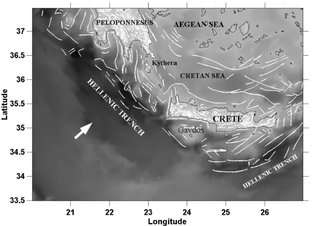
The SW segment of the Hellenic Arc (34◦_{N – 37.5}◦_{N, 20}◦_E – 26◦_{E) is the most active plate margin of the Mediterranean} area, with correspondingly high seismicity and relatively fre-quent occurrence of large earthquakes. The main geotectonic features of the area are shown in Fig. 1, the most dominant of which is the Hellenic Trench, where the eastern Mediter-ranean oceanic lithosphere (front part of the African plate) is subducted under the Aegean microplate. To the north of the trench, the Hellenic Arc (Peloponnesus – Kythera – Crete) comprises the accretionary prism and farther north, other typ-ical elements of a subduction system are seen, namely the southern Aegean trough (Cretan Sea) and parts of the vol-canic arc – Milos and Thera (Santorini).

As mentioned above, the SW Hellenic Arc and Trench sys-tem generates large shallow- and intermediate-depth earth-quakes many of which have been reported since the early historic times. Magnitudes of up to 8.0 have been reported in the literature, (e.g. Papazachos, 1990; Papazachos and Papazachou, 1997). Although such figures may have been overestimated, (some of them were drawn on the basis of an-cient and medieval archival data), they still signify the great seismogenetic potential of the area.

With such a setting and history, the area has attracted at-tention and in the recent past, a number of predictions of large events appeared in the literature. A large shallow earth-quake of M7.7±0.5 was forecasted by Wyss and Baer (1981) to take place, between 1980 and 1991, in a quiescent zone northwest of Crete and along the Hellenic Arc (rupture length 100±50 km). A similar prediction was also made by Papaza-chos and Comninakis (1982), but a with a narrower time win-dow. Such an event has yet to occur. The failure can partly be attributed to the fact that earthquake epicentres determined by the theretofore network of the Geodynamics Institute of the National Observatory of Athens and thought to lie south of the Aegean plate boundary in the African plate, were in fact located an average of 60 km to the NE (Papadopoulos et al., 1988). Such problems would, of course be

detrimen-Fig. 1. The principal geotectonic and structural features of the SW Hellenic Arc and Trench system.

tal to any prediction made with methods requiring precise earthquake location data, as does the quiescence hypothesis. Ferraes (1985) reached a similar conclusion, but with the oc-currence of the main event estimated for the decade 1992 to 2002. This period is also about to expire.

Sequences of accelerating seismic release rates have also been investigated and identified in the WSW Hellenic Arc. Prior to the appearance of the time-to-failure model, in a series of well constrained observational studies Papadopou-los (1986, 1988a, 1988b) identified a number of acceler-ating sequences comprising intermediate magnitude events (MS ≥5.2) and has also claimed the successful prediction of the 13 September 1986 Kalamata earthquake. Retrospective analysis of intermediate magnitude seismicity was conducted by Papazachos and Papazachos (2000) and Papazachos and Papazachos (2001), on the basis of the accelerating time-to-failure model. These authors concluded that during 1948– 1957, the four large, shallow main-shocks to have occurred in the area, (9 February 1948, 35.5◦N, 27.2◦E, M = 7.1; 17 December 1952, 34.4◦N, 24.5◦E, M = 7.0; 9 July 1956, 36.6◦N, 26.0◦E, M = 7.5; 25 April 1957, 36.5◦N, 28.8◦E, M = 7.2), were preceded by accelerating seismicity, typi-cally in the range M4.5–6.8. In a most recent publication, Papazachos et al. (2002) report of a similar accelerating seis-micity pattern that has started several years ago and currently develops in the area. By modelling this sequence, they expect a magnitude 6.8±0.5 event to take place up to year 2004.4.

Our interest in the area was motivated by our desire to test and evaluate the predictive capability of the CP model in a region that has been shown to generate accelerating precur-sory sequences, also given its history of large earthquakes and “failed” or “successful” predictions, and the absence of a strong earthquake in the entire southern Aegean area dur-ing the past few decades, which may indicate that such an event may be due. Unlike Papazachos et al. (2002), who fo-cus on intermediate magnitude scale pre-shock activity, we include smaller events in the analysis (down to the magni-tude of completeness), on the premise that SOC and CP pro-cesses are independent of scale and therefore, accelerating sequences should appear consistently at all magnitudes.

Independently of Papazachos et al. (2002), we have iden-tified approximately the same areas of accelerating seismic release rates. In addition, we have also identified adjacent areas of decelerating seismic release rates. The configura-tion of the accelerating and decelerating sequences hint of a causal relationship between them, which we have tried to explain in terms of stress transferred by certain fault config-urations preparing to rupture the area. Supposing that the CP/time-to-failure model does indeed describe the observed seismicity changes in the area, an obvious benefit of such an endeavour is our ability to better constrain and model hazard and risk from such an event by estimating the size, orienta-tion and rake of the seismic source, as well as its average dis-tance from inhabited or industrial areas. Our investigations

Fig. 2. The catalogue of the Geodynamics Institute of the National Observatory of Athens, spanning the period 1 January 1965 – 30 April

2002. The magnitude scale is ML(see text for details). The study area is defined by the grey shaded rectangle.

and results are reported in the following.

2 Data conditioning and analysis procedures

The seismicity data used in this study are taken from the raw catalogue of the Geodynamic Institute of the National Obser-vatory of Athens (GI-NOA, http://www.gein.noa.gr/services/ cat.html) and span the period 1 January 1966 – 10 April 2002 (Fig. 2). This is the most detailed (but not most accurate) cat-alogue of Greek seismicity and contains upwards of 42 000 events.

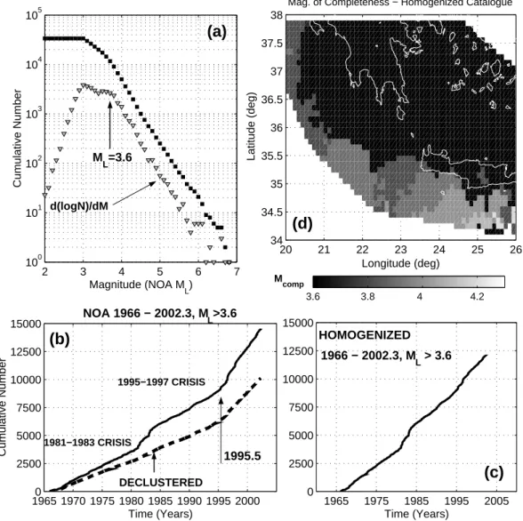
The GI-NOA reports local magnitudes (ML) and its cata-logue is neither homogeneous nor complete. To investigate completeness, in Fig. 3a we present the frequency-magnitude statistics. Clearly, there are two magnitude bands with ap-parently different scaling, as is also obvious in the derivative d(logN)/dM (triangles). The first is ML≈3–3.6; the second is ML ≈ 3.7–6.9, with the upper end being the maximum observed during the studied period 1966–2002.3. We have insufficient information to decide whether this change is nat-ural or artificial, due to differences in magnitude reporting

between the larger and the smaller events. At any rate, for apparent reasons we conclude that a useful and reliable lower limit of completeness is MS =3.7, i.e. the lower bound of the larger magnitude band.

To investigate (in)homogeneity, in Fig. 3b we present the cumulative number curve for magnitudes ML ≥ 3.6 (solid line); this subset contains approximately 14 800 events. Sev-eral time-local changes of seismicity rates exist, the two most prominent of which appear to coincide with periods of seis-micity crises, (1980–1983 and 1995–1997), and can thus be attributed to the large number of aftershocks reported. There also appears to be a persistent rate change after year 1995. To decide what is what we declustered the catalogue using the method of Reasenberg (1985). This identifies in a series of earthquakes, which are correlated by means of Omori’s law within a given radius and time window and replaces them with an equivalent event at the location of the leading largest earthquake, with magnitude corresponding to the total en-ergy released during the sequence. In this way, the num-ber of main events (hence background seismicity rates) re-mains intact. The cumulative number curve for the declus-tered catalogue is shown in Fig. 3b (dashed line). As

antici-2 3 4 5 6 7 100 101 102 103 104 105 Magnitude (NOA M_L) Cumulative Number 3.6 3.8 4 4.2 20 21 22 23 24 25 26 34 34.5 35 35.5 36 36.5 37 37.5 38 Longitude (deg) Latitude (deg)

Mag. of Completeness − Homogenized Catalogue

1965 1970 1975 1980 1985 1990 1995 20000 2500 5000 7500 10000 12500 15000 Time (Years) Cumulative Number NOA 1966 − 2002.3, M L>3.6 1965 1975 1985 1995 2005 0 2500 5000 7500 10000 12500 15000 Time (Years) M L=3.6 d(logN)/dM 1981−1983 CRISIS 1995−1997 CRISIS DECLUSTERED 1995.5 HOMOGENIZED M comp

(a)

(b)

(c)

(d)

Fig. 3. (a) The frequency - magnitude statistics of the NOA catalogue. (b) The cumulative number curves of the raw NOA catalogue (solid

line) and the declustered NOA catalogue (dashed line), above the magnitude of completeness (ML≥3.6). (c) The cumulative number curve

of the homogenised NOA catalogue above the magnitude of completeness (ML≥3.6). ((d) Map of the magnitude of completeness, based

on the homogenised NOA-ML catalogue. Grid dimension is 0.1◦square and calculations were based on a minimum of 200 events around each grid point.

pated, the time-local rate changes due to the seismicity crises have disappeared but the persistent rate change has been con-firmed. It begins on year 1995.5 approximately, as identified with Habermann’s GenAS procedure (Habermann, 1983). To quantify the rate change, we applied the method of Z´u˜niga and Wyss (1995) to compare the frequency-magnitude statis-tics and rates for two non-overlapping periods, P 1 = 1970– 1995.3 and P 2 = 1995.4–2002.2. We have thus determined that between the two periods the magnitudes are related as

MP2=0.85 · MP1+0.71. (4)

It appears that the post-1995 rate change can reasonably be attributed to a corresponding change in the procedure of mag-nitude reporting at NOA. Indeed, as of January 1995, NOA began upgrading its entire network from a purely analogue system based on leased line telemetry, first to a hybrid and

then to a digital system based on leased data line telemetry. It is conceivable that small changes in magnitude calculations may have resulted from small changes in the recording and reading of the seismograms. Unfortunately, and since there has not been any performance analysis of the NOA network before and after the upgrade, there is no way of pinpointing the factors that effected the changes. Nevertheless, by using Eq. (4) it is possible to adjust the magnitudes of either pe-riod with respect to the other and thereby restore homogene-ity to the catalogue. Herein, we have chosen to correct the magnitudes of P 2 with respect to P 1, which is considerably longer in duration. Figure 3c presents the cumulative num-ber curve of the homogenised catalogue, which after the due adjustment for completeness contains nearly 12 000 events with ML≥3.6.

5

10

15

20

3

4

5

6

7

3

4

5

6

7

8

Local Magnitude (NOA)

Surface Magnitude (ISC)

3

4

5

6

7

3

4

5

6

7

8

Average Local Magnitude (NOA)

Surface Magnitude (ISC)

1184 EVENTS

M

S

= 1.687*M

− 3.35

(a)

(b)

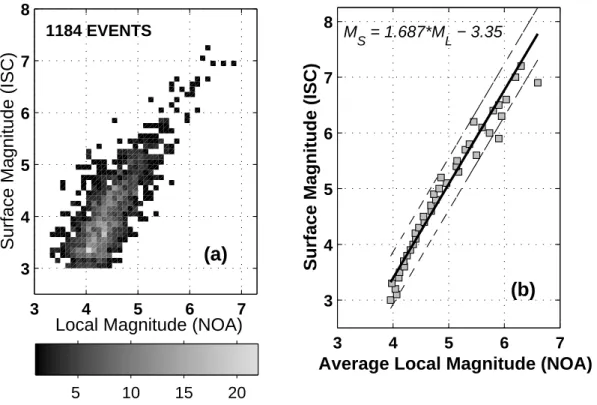
Fig. 4. (a) Graphical representation of NOA-MLvs. ISC-MS magnitudes for 1184 common events between 1 January 1978 and 30 April

2000. The shading represents the density of multiple mappings per magnitude interval. (b) The squares represent the row-wise NOA-ML

weighted average magnitude vs. ISC-M_S, together with the best fitting straight line and 95% confidence limits.

in completeness may exist over an extended area. To check this problem in our study area, we compiled a magnitude of completeness map, calculated as per Fig. 3a, on a 0.1◦square grid, using a minimum of 200 events around each grid point. The result is shown in Fig. 3d. As evident, completeness de-teriorates from ML≈3.6 to ML≈3.9–4 toward the periph-ery of the Hellenic Arc and Trench system. In consequence we consider that ML =3.9 should rather be adopted as the absolute magnitude threshold for the ensuing analysis.

The energy Ei(t )required by Eq. (3) can be estimated after Gutenberg and Richter (1956) as

log₁₀Ei(t ) =4.8 + 1.5 · MS, (5a) which yields

log₁₀ε(t ) =log₁₀pEi(t ) =2.4 + 0.75MS. (5b) Kanamori and Anderson (1975) have shown that Eq. (5a) is consistent with what is expected theoretically for a classical crack model with a constant stress drop. The stress drop does not vary significantly with earthquake size (e.g. Kanamori and Anderson, 1975; Hanks 1977), at least down to seismic moments of the order 5 · 1018ergs, (MW ∼3 or MS ∼1.5, e.g. Hanks, 1977). Thus, Eqs. (5) comprise energy – mag-nitude scaling laws applicable over a broad range of magni-tudes.

Since NOA reports local magnitudes, it is necessary to convert ML to MS. To address this problem we have used the subset of the International Seismological Centre (ISC)

catalogue that reports MSmagnitudes, for the area of Greece and adjacent territories, as shown in Fig. 1 (ISC On-line Bul-letin, http://www.isc.ac.uk/Bull). The NOA-MLand ISC-MS catalogues contain 1184 common events between 1/1/1978 and 30/4/2000. Figure 4a is a graphical representation of NOA-ML vs. ISC-MS. If j is a discrete variable spanning the MLmagnitude range and k is a corresponding variable over the MS magnitude range, then Fig. 4a shows a density matrix whose elements represent the number of ML mag-nitudes that map onto a given MS magnitude in the sense N (k, j ) = {ML(j )} → MS(k), with {.} denoting an ensem-ble. The two magnitude scales are apparently linearly corre-lated for MS >3 and ML>3.4–3.5 and up to magnitudes of the order of 7. However, it is not recommended to compute a LS model of their relationship with the raw ML−MSdata set because there is considerable redundancy, i.e. multiple map-pings of ML(j )onto MS(k), and heavy bias toward the lower magnitude ranges, thus producing a grossly unbalanced data set. To circumvent this problem, we chose to model the re-duced data set < ML(k) > −MS(k), where

< ML(k) >= X j ML(j )∗N (k, j )/ X j N (k, j )

is the row-wise weighted average of the MLpopulation and is shown in Fig. 4b together with the 95% confidence lim-its. Using a robust weighted LS regression with a re-descending bisquare influence function on the reduced data set, we obtained the best fitting line

0.3 0.4 0.5 0.6 0.7 0.8 0.9 1

Easting (km)

Northing (km)

Curvature

A

B

Peloponnesus

Crete

Gavdos

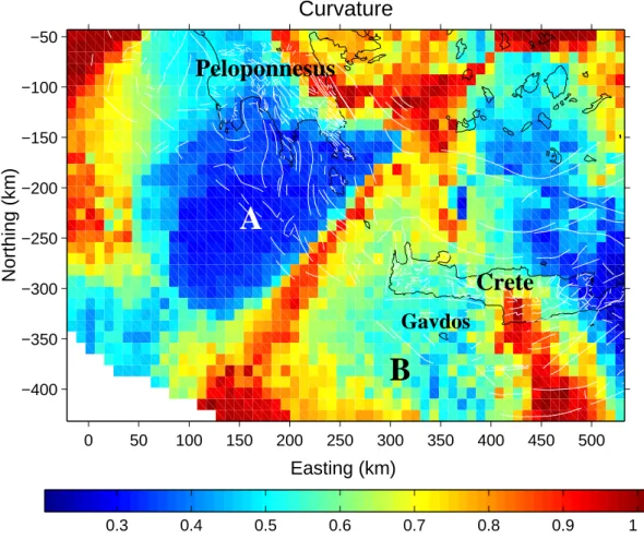
Fig. 5. Map of the curvature at the optimal radius, C(Rc). Grid dimension is 0.1◦.

which can be used to convert NOA-MLmagnitudes to ISC-MS and is also shown in Fig. 4b. Let us also point out that the MLmagnitudes reported in the NOA catalogue ap-pear to be biased downwards by about 0.5 in the range 3.5 ≤ ML ≤ 6.5, probably due to the low static magnifi-cation of the WoodAnderson instrument at NOA (e.g. see Margaris and Papazachos, 1999). This bias is compensated for in Eq. (6). Finally, we note that a linear relationship of the form (6) was also reported by Papazachos et al. (1997), but it was derived from a data set much smaller than the one we used herein.

The identification of power-law behaviour in seismic re-lease rates is rather straightforward: the cumulative Benioff strain vs. time for earthquakes within a circle of radius R is modelled with the time-to-failure power-law relation (3), us-ing a Hedgehog non-linear optimisation procedure operatus-ing on the L2norm. At the critical time tc, Eq. (3) reduces to ε(tc) = K. Therefore, at any t → tc, Eq. (5b) can be used to obtain a predicted magnitude as

ˆ

MS =(log10[K − ε(t )] −2.4)/0.75. (7) Following Bowman et al. (1998), the performance of the power law fit against the null hypothesis of constant seismic release rate, is quantified by defining a curvature parameter C=(Power law fit RMS)/(Linear fit RMS),

such, that when the data are best described by a power-law curve, the RMS error will be small compared to the RMS er-ror of the linear fit and C will also be small. Such modelling of the cumulative Benioff strain is repeated over a set of ex-panding concentric circles. The radius Rc such that C(Rc) = min{C(R)} and the corresponding model parameters are deemed optimal and stored. The procedure is applied on a regular geographic grid and maps of the optimal curvature, critical exponent, critical time and predicted magnitude are compiled. In this way it is possible to identify regions of ac-celerating seismic release, which can be further investigated with more advanced techniques.

3 Results

Time-to-failure modelling is carried out on a 0.1◦_{square grid} and the results are presented in Figs. 5 and 6. Figure 5 is a map of the curvature at the optimal radius, C(Rc), where def-inite evidence of power-law evolution in seismic release rates can be observed. The lowest curvature values (of the order of 0.3) are observed at the Hellenic Arc and Trench, to the south of Peloponnesus (Area A). In addition, relatively low curvatures (0.4–0.6) are observed to the south of W. Crete, around Gavdos island, within the Hellenic Arc (Area B). A third area of low curvatures (of the order 0.3–0.4) observed

0.2 0.4 0.6 0.8 1 1.2 1.4 1.6 1.8 2

Easting (km)

Northing (km)

Critical Exponent

Fig. 6. Map of the critical exponent at the optimal radius, n(Rc). Grid dimension is 0.1◦.

around eastern Crete will be the subject of an independent study and will not concern us here. It should be noted, however, that unless otherwise constrained, good power-law models of seismic release rates can be obtained either when they are accelerating (the critical exponent n < 1) or decel-erating (n > 1). By inspecting the corresponding map of the optimal critical exponent n(Rc)– which is shown in Fig. 6, it is possible to distinguish between accelerating and decel-erating sequences. The distribution of the critical exponent shows a well structured four-leaf pattern, in which quadrants with exponents greater than unity and quadrants with ex-ponents smaller than unity alternate, separated with almost sharp boundaries. Closer inspection reveals that the Area A of low curvatures is associated with critical exponents n(Rc) of the order of 0.2–0.35, consistent with expectation for CP behaviour. Conversely, the Area B is associated with crit-ical exponents n(Rc)of the order of 1.4–1.8 and relatively strong deceleration. Note however that in the context of the CP model, Eqs. (1) and (3) have definite physical meaning only for accelerating sequences; they have uncertain physics and no predictive value in the case of decreasing seismic re-lease rates. In consequence, the estimated critical times and predicted magnitudes are significant only in the neighbour-hood of Area A. In order to have some idea about the stability of the modelling procedure, we compute the means and

stan-dard deviations of predicted magnitudes and critical times of models computed at the grid nodes of Area A, subject to the constraints C(Rc) ≤ 0.4 and 0.15 ≤ n(Rc) ≤ 0.35. The resulting populations contain upwards of 200 realisations of the relevant parameters, from which < ˆtc >=2003.6 ± 0.55 and < ˆMS>=7.1 ± 0.4.

The results are quite stable and consistent. Nevertheless, the picture may not be as bright – if we attempt to derive the same parameters from a different starting point. Specif-ically, another method of predicting the magnitude involves the size of the scaling region around the culminating event. On the basis of CP theory, Bowman et al. (1998) conclude that log R ∝ 0.5 M and also provide an empirical linear rela-tionship in which log R ∝ 0.44 M. Papazachos and Papaza-chos (2000) provide for the Aegean area, the relationship log R = 0.41 M − 0.64, where M is the moment magnitude. The mean optimal radius (Rc)at Area A is 102±14.4 km (grid nodes with C(Rc) ≤ 0.4). Using either relationship above, and with due adjustment of the moment to surface magnitudes, we find ˆMS = 6.3 − 6.6. Thus we run into an apparent contradiction that should not be: Predicted magni-tudes computed by direct modelling are significantly higher than predicted magnitudes computed indirectly, from empir-ical relationships based on observational studies. We also note that the problem persists, no matter how one doctors

Fault relaxed, Regional Stress relaxed

fault

Fault stresses up / regional field stresses up

fault

Stress−up continues ...

fault

Stress−up nearing point of failure

fault Failure Threshold Acceleration Deceleration

(a)

(b)

(c)

(d)

Fig. 7. Schematic representation of a physical model, whereby the observed characteristics of accelerating seismic release rates can be

understood in terms of simple elastic rebound and stress transfer from a fault, to a region already subjected to stress inhomogeneities. (a) At the beginning of the cycle, the regional stress is relaxed and local inhomogeneities produce local instabilities. (b–d) With time, at some areas positive stress transfer and build up causes progressively more local failures (acceleration). Conversely, at areas of negative stress transfer, progressively fewer local failures are expected (deceleration).

with the size of the optimal radius or the apparent size of Area A.

CP theory does not make any particular predictions about the configuration or shape of the critical region around the approaching large earthquake. In fact, it was initially thought that the critical region extends everywhere around the future epicentre and hence the earlier methods of searching for ac-celeration in circular domains (e.g. Varnes, 1989; Bufe and Varnes, 1993; Bufe et al., 1994; Sornette and Sammis, 1995; Brehm and Braile, 1998, 1999; Bowman et al., 1998, and others). If this was the only physical possibility, then the contradiction would be bad news as it would point toward inconsistencies, either in the theory, or in the observational studies, or in both.

The physical models of accelerating seismic release may provide an explanation and particularly so, the idea of Bow-man and King (2001) that the observed characteristics of dis-tributed accelerating seismicity may be produced by increas-ing tectonic stress in a region already subjected to stress in-homogeneities. Unlike methods using circular or elliptical regions to search for accelerating seismicity, this approach

defines the critical region in terms of the stress field required to rupture a fault with a specified orientation and rake. This model can possibly explain observations of decelerating seis-micity as well, because during earthquake preparation cycle, stress does not evolve uniformly around the fault. Rather, there exist “bright spots” where stress is increasing by trans-fer from the fault, and shadows where stress may even be relaxing. The configuration of these volumes depends of the nature and geometry of the fault and whereas acceleration may be observed in stress bright spots, deceleration may be expected in stress shadows. This concept is schematically illustrated in Fig. 7. At the beginning of the cycle, the re-gional stress is relaxed due to the stress shadow of a previous large earthquake and local stress inhomogeneities may rup-ture local faults when their level exceeds some failure thresh-old (Fig. 7a). With time, the regional stress increases at some areas, where progressively more local stress inhomogeneities are likely to exceed the failure threshold and rupture, produc-ing acceleration of seismic release rates (Figs. 7b–d). Con-versely, at areas of stress decrease, progressively fewer local inhomogeneities are likely to rupture; this amounts to an

ap-−0.25 −0.2 −0.15 −0.1 −0.05 0 0.05 0.1 0.15 0.2 0.25

Easting (km)

Northing (km)

Failure stress at 20 km

x 10

Pa

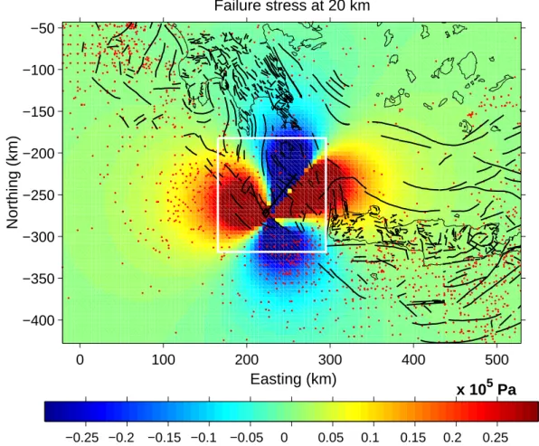
Fig. 8a. Failure stress due to a NE-SW oriented strike – to oblique-slip fault (thick black line, ϕ = 35◦, δ = 80◦, λ = −35◦), capable of producing an MS = 7.1 earthquake in a homogeneous medium with Young’s modulus 7 · 107Pa. Failure stress is defined as (σ1+σ3)/2

and the calculation is taken to the depth of 20 km. The white rectangle encloses the area where a family of similar faults produces a similar stress distribution, which may explain the observations of accelerating seismic release rates. The colour-code of stress variations represents the interval −3 · 104Pa to +3 · 104Pa. Red dots are earthquake epicentres.

parent decrease of seismic release rates. At this point we note that hitherto observational studies have focused on accelera-tion, since this is the main prediction of the CP model. In general, non-linear deceleration has not been researched as a possible precursory effect, let alone that even the precursory quiescence hypothesis does not predict such a phenomenon. Herein we observe both effects in such a well structured and organised manner, which is strongly suggestive of a causal relationship.

To investigate whether the above hypothesis may explain our observations, we define a fault with a given size, orienta-tion and rake and back-slip it in order to determine the areas of stress increase/decrease prior to the earthquake, using the 3-D boundary element fault modelling program 3D-DEF by Gomberg and Ellis (1994). The Earth’s crust is necessarily assumed to be homogeneous and the geometry of the fault plane is kept simple, inasmuch as there is practically no in-formation on the characteristics of real fault planes capable of rupturing at the study area.

After several trials, we concluded that both accelerated and decelerated seismic release patterns can possibly be

ex-plained with a family of NE-SW, left-lateral, strike-slip to oblique-slip faults, capable of producing earthquakes with magnitudes MS ∼7. These faults are located within the rect-angle shown in Figs. 6 and 8a. A representative member of this family produces the failure stress distribution of Fig. 8a, where failure stress is defined as (σ1+σ3)/2. It has orienta-tion ϕ = 35◦_{, dip δ = 80}◦_{, rake λ = −35}◦_{, depth of burial} 5 km and is capable of producing an MS =7.1 earthquake in a homogeneous medium with Young’s modulus 7 · 1010Pa. As evident, stress increase is observed in area A where accel-eration is also observed and stress decrease in area B where deceleration is observed.

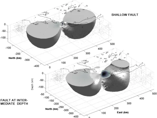
We emphasize that no other significantly different fault ge-ometry can account for all of the observations! However, we also note that the depth to the fault cannot be adequately con-strained. Whether it is outcropping at sea-bottom or is buried at a depth of, say, 50 km, the fault will produce very similar patterns of stress bright spots and shadows. To illustrate this point, in Fig. 8b we present the 1 kPa iso-surfaces of stress bright spots for two faults. The first is a shallow fault, exactly as per Fig. 8a. The second has exactly the same geometry,

Fig. 8b. The upper left panel shows the 1 kPa iso-surface (positive stress lobes) due to a shallow fault with characteristics ϕ = 35◦, δ = 80◦, λ = −35◦, capable of producing an earthquake of magnitude MS = 7.1. The lower right panel shows the 1 kPa iso-surface due to an

intermediate depth fault (buried at 50 km), with identical geometry. The crustal volumes within the surface experience stress increase greater than 1 kPa. Earthquakes hypocentres have also been superimposed (black dots).

but is buried at the intermediate depth of 50 km. Earthquake hypocentres have also been superimposed (black dots). As can be seen, in both cases the volume of stress increase (in-side of the iso-surfaces) includes all earthquakes of area A, with differences concerning only a handful of events. Sim-ilarly the volume of stress decrease includes all earthquakes of area B, again with very minor differences. Without addi-tional data, it is rather difficult to infer about the depth of the fault at this point in time.

Another important question is of whether it is possible to have this kind of strike-slip fault in the SW Hellenic Arc, which comprises the accretionary prism of a subduction zone. Hitherto work on fault plane solutions of 20th century earthquakes has not observed evidence of strike-slip fault-ing at shallow crustal depths. There is, however, evidence of NE-SW strike-slip faulting at intermediate depths (a classi-fication of known focal mechanism in the Aegean area can be found in Papazachos and Papazachou, 1997). However, it has to be noted that reliable focal mechanism data exist for the last third of the 20th century only. It is more than certain that within this very short period, not one large fault has ruptured. Likewise, not all faults capable of producing intermediate-size earthquakes with all possible permissible mechanisms have ruptured. The available data sample is sim-ply not large enough to allow definite conclusions and com-prises (at best) a large sample of the existing possibilities. Thus, while an intermediate depth NE-SW strike-slip rupture with the detected characteristics is altogether possible, a

rel-atively shallow fault cannot be ruled out, as it may comprise a transcurrent structure facilitating the SW-ward motion of the Aegean plate and the tectonic setting of the area does not preclude it.

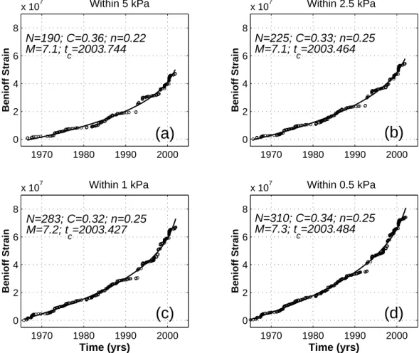
Returning to our analysis and in order to provide some numbers and a measure of the acceleration rates in the areas of stress increase, Figs. 9a–d illustrate models of the acceler-ating seismic release at Area A, at the west positive lobe of the stress field of Fig. 8a, computed with earthquakes laying inside the 5 kPa contour (Fig. 9a), 2.5 kPa contour (Fig. 9b), 1 kPa contour (Fig. 9c) and 500 Pa contour (Fig. 9d). It is evident that while the sampled area increases from 16 000 to over 82 000 km2, and the number of earthquakes modelled increases from 190 to 225, 283 and 310, respectively, the predicted parameters remain remarkably stable: MˆS is 7.2, 7.1, 7.2 and 7.3, respectively, and ˆtc is 2003.744, 2003.464, 2003.427 and 2003.484, respectively, all in agreement with the results obtained above. At the same time, the critical ex-ponent remains at the level of 0.25 throughout, as predicted by the spinodal instability model of Rundle et al. (2000), in-dicating that at this point in time, this particular fault net-work acts like a CP system at the verge of a first order phase transition. The remarkable consistency of the results of Figs. 9a–d can possibly be due to the fact that all earth-quakes used for modelling may still lay inside the correlation length of the stress-stress interactions stimulated by the fault. In other words, the boundary of the critical scaling region is still beyond the 500 Pa contour. Indeed, the radius of a

cir-1970 1980 1990 2000 0 2 4 6 8 x 107 Benioff Strain Within 5 kPa 1970 1980 1990 2000 0 2 4 6 8 x 107 Within 2.5 kPa Benioff Strain 1970 1980 1990 2000 0 2 4 6 8 x 107 Time (yrs) Benioff Strain Within 1 kPa 1970 1980 1990 2000 0 2 4 6 8 x 107 Time (yrs) Benioff Strain Within 0.5 kPa

N=190; C=0.36; n=0.22

M=7.1; t

=2003.744

N=225; C=0.33; n=0.25

M=7.1; t

=2003.464

N=283; C=0.32; n=0.25

M=7.2; t

=2003.427

N=310; C=0.34; n=0.25

M=7.3; t

=2003.484

(a)

(b)

(c)

(d)

Fig. 9. Models of accelerating seismic release at Area A, in the western positive lobe of the stress field, computed with earthquakes (a) within

the 5 KPa contour, (b) within the 2.5 KPa contour, (c) within the 1 KPa contour, (d) within the 500 Pa contour. In each graph the cumulative Benioff strain is shown with small open circles. The continuous line indicates the best fitting power-law model.

1965 1970 1975 1980 1985 1990 1995 2000 2005 0 1 2 3 4 5 6 7 8 9x 10 7 Time (yrs) Beniof Strain C=0.6; N=286 n=1.6

(e)

Fig. 9e. A model of decelerating seismic release at Area B, in the

eastern negative lobe of the stress field, computed with earthquakes inside of the −5 KPa contour.

cle with area equivalent to the area of the 500 Pa contour is

approximately 162 km. Upon using the radius - magnitude scaling relationships quoted above, we find that the culmi-nating event will have magnitude ˆMS = 6.95–7.1, slightly smaller, but in excellent agreement with the results of mod-elling. Quite reasonably, if the above explanation of our ob-servations corresponds to true Earth processes, it will be very difficult to determine the exact extent of the scaling region, because at some point, it will interact with the scaling re-gions of other major faults. Finally, Fig. 9e shows a model of the decelerating sequence in Area B, constructed with earth-quakes inside of the −5 KPa contour. This is shown only for the sake of completeness, since Eq. (3) has no predictive value for decelerating sequences.

In the light of the above evidence, it is possible to ex-plain why it was not possible to calculate consistent mag-nitudes from the size of the circular optimal radii in Area A. The relatively small size of the optimal radii (and of Area A thereof), can be explained as result of data statistics. For so long as the search radius remained inside the true scaling region defined by the non-circular area of increasing stress, the time-to-failure model would return consistent estimates of the critical time and predicted magnitude. However, once

1990 1992.5 1995 1997.5 2000 2002.50 0.2 0.4 0.6 0.8 1

Time (yrs)

Curvature

Time (yrs)

Predicted Magnitude

Time (yrs)

Critical Time

Time (yrs)

Critical Exponent

Fig. 10. Unconditional running forecast of an accelerating sequence. Computations are carried out at 12 cut-off times between 1990 and

2002, using the earthquakes located in Area A, inside of the contour C(Rc) <0.4 of Fig. 5.

the search radius grew so large, as to surpass the boundaries of the scaling region, the contribution of uncorrelated earth-quakes would quickly destroy the power-law behaviour of the cumulative Benioff strain: the true size of the scaling region and any associated parameters would be misestimated.

Albeit remarkable, these results should be viewed with due caution. The fault model is a simple plane rupturing a homo-geneous continuum and cannot be expected to account for all the details of the observations; these result from the inter-play between the material properties and stress distribution in the real crust (which are unknown and cannot be mod-elled with precision), and the statistics and constitution of the earthquake sample processed at each grid point. More-over, the geometry of the NOA network at the SW Hellenic Arc is such, that systematic, sometimes considerable loca-tion errors may be expected (e.g. Papadopoulos et al., 1988). The situation has improved in the past decade but the prob-lem is still not solved. While this is certainly a significant disadvantage, it does not have a detrimental effect on deter-mining the approximate extent of the scaling region, as this comprises a rather large crustal volume over which the ob-servations are integrated. It may, however, complicate the modelling of faults capable of producing these changes.

4 Discussion and conclusions

We have detected and investigated power-law acceleration of seismic release rates in the SW Hellenic Arc, consistent with the Critical Point earthquake model. Our observations are consistent with physical models of the seismic cycle, which predict such an effect as the result of regional stress in-crease and the establishment of long-range stress-stress cor-relations over the fault network involved in the preparation of a large event (Heimpel, 1997; Ben-Zion and Lyakhovsky, 2001; Bowman and King, 2001; King and Bowman, 2001). Moreover, our observations are consistent with the view of the power-law acceleration of seismic release as a particular type of self-organising CP systems undergoing a repetitive series of first order phase transitions (spinodal instabilities), as discussed in Rundle et al. (2000).

The model of King and Bowman (2001) on one hand and the theory of Rundle et al. (2000) on the other, while very different in approach and formulation, share a very impor-tant and defining characteristic. King and Bowman (2001) base their model on the decay of a stress shadow which is perturbed by fractal noise representing local stress inhomo-geneities. The number and size of model events increases

due to the corresponding increase in the number and size of stress patches above a failure threshold and this can be in-terpreted as an effective increase of the correlation length. Spinodal phase transitions are possible in systems with long-range interactions, which act to stabilise them against small fluctuations. Accordingly, Rundle et al. (2000), show that the stress-stress correlation length increases proportionally to the inverse square root of the time-to-failure. This of course, amounts to dynamic self-organisation of the fault network. Thus, in both cases the acceleration of seismic release is a consequence of increasing the span of interactions through the activated fault network.

As indicated by Huang et al. (1998), the critical nature of large events results from the interplay between the long-range stress-stress correlations of the self-organised critical state and the hierarchical fault structure in such a way, that hierarchical rupture at a given level is like a critical point to the lower levels. Thus, triggering of distributed failures in the area of stress increase may cause stress redistribution that triggers more faults at neighbouring regions, and so on. Such interactions between small events smooth the stress field and establish long-range stress correlations over the critical area, producing with time hierarchical ruptures: the many-fault in-teractions may account for the power-law behaviour of the accelerating seismic release with a critical exponent equal to 0.25. We shall refrain from pursuing this discussion any far-ther, inasmuch as we intend to present a thorough theoretical development of the topic in a follow-up work.

It appears that our analysis has produced all the elements required for earthquake prediction, albeit of medium-term: Location, (SW Hellenic Arc, between Crete and the Pelopon-nesus), time (2003.6±0.6) and size of the event (7.1±0.4). In addition, if the physical model upon which we have based the interpretation is correct, we may have even determined the main characteristics of the fault that is going to rupture (ϕ ≈ 35◦, δ ≈ 80◦, λ ≈ −35◦), albeit not its burial depth. For the given geotectonic setting, data and analysis proce-dures, the predicted parameters appear to be fairly reason-able. However, are they? Is this really a prediction?

It is difficult to give a clear cut answer. Time-to-failure modelling of accelerated seismicity is a relatively new field of study with few cases-histories from which to draw expe-rience, most of which in fact comprise retrospective analy-ses of past earthquakes. Still, very little is known as to the development of real-time situations and their probability of success or failure. Also note that the scaling law (3) is es-sentially the result of a renormalisation process. Its under-pinning is the concept of a scaling region in the time and space before a large rupture, assuming that the process of failure at a small spatial scale and temporarily far from a global event can be remapped (renormalized) to the process of failure at a larger scale and closer to the global event. By this re-mapping, the area of the pre-seismic release scales with the magnitude of the earthquake, which is like saying that the total energy released prior to global failure scales with the energy to be released at global failure. Its useful-ness “... is based on the existence of a scale invariance or

self-similarity of the underlying physics at the critical point, which allows one to define a mapping between physical scale and distance from the critical point” (Sornette and Sammis (1995). In consequence, when a new element is added, (i.e. a large schock), the sequence is renormalized and the pre-dicted parameters may change, sometimes significantly.

To reassert this point, in Fig. 10 we illustrate the uncon-ditional running forecast of an accelerating sequence, car-ried out at 12 cut-off times between 1990 and 2002.2, us-ing the earthquakes located in Area A, within the contour C(Rc) < 0.4 (Fig. 5). The evolution of the acceleration, from barely significant to fully developed power-law be-haviour is evident in the reduction of curvature from 0.8 to 0.4. The critical exponent remains at the level 0.2–0.3 and the predicted magnitude is very stable. However, the esti-mated critical time changes from year 2000.2 to year 2004, although it is apparently trying to stabilize during the latter times of the sequence. Thus, at least one element of the pre-diction is unstable and we have difficulty in telling how the sequence will develop in the future.

Yet another difficulty arises from the fact that even if en-ergy is currently building up in the form of deformation at the critical area, it is not at all necessary that a large earth-quake will occur as soon as the activated system enters the critical state (at time tc). The CP model merely predicts that past this time an earthquake is possible. As stated in the in-troduction, the time of the large event may depend on several uncertain factors pertaining to the nucleation process, which may have significant time dependence. Moreover, the stored energy may be dissipated with aseismic (low moment release rate) event(s) or with a series of smaller earthquakes. Again, the absence of a concrete case history complicates our abil-ity to make solid inferences. For all the reasons above, and given the little experience with the method on the interna-tional level, it is hard to assert a prediction.

On the upside, we note that the results are based on a phys-ical, not a statistical model. If it represents real Earth pro-cesses, then the evidence is telltale and compelling. Note also that if the prediction of CP theory is correct, that pre-shock magnitudes get progressively larger with approaching to fail-ure, then recent seismicity patterns indicate that the critical point may not be far. To this effect, we note that Papaza-chos et al. (2002) have also made very similar observations and predictions for the same area, based on a quite different catalogue from which only magnitudes greater than 5 were used, by implementing a significantly different detection and estimation procedure. It appears that at this point in time, the only answer is continuous monitoring of seismicity changes, persistent vigilance for additional evidence that will signal the approach of the critical time and good luck, whatever is the meaning of “luck” in a situation like this! The bottom-line is that we have detected and documented evidence of a self-organised fault network possibly working its way to-ward instability, which is strongly suggestive of a true phys-ical process. If not, then we have probably come across a synod of truly diabolic coincidences!

References

All`egre, C. J. and LeMou¨el, J. L.: Introduction of scaling techniques in brittle failure of rocks, Phys. Earth Planet Inter., 87, 85–93, 1994.

Ben-Zion, Y. and Lyakhovsky, V.: Accelerated seismic release and related aspects of seismicity patterns on earthquake faults, Pure Appl. Geophys., in press, 2002.

Bowman, D. D., Ouillon, G., Sammis, C. G., Sornette, A., and Sor-nette, D.: An observational test of the critical earthquake con-cept, J. Geophys. Res., 103, 24 359–24 372, 1998.

Bowman, D. D. and King, G. C. P.: Accelerating seismicity and stress accumulation before large earthquakes, Geophys. Res. Lett., 38 (21), 4039–4042, 2001.

Brehm, D. J. and Braile, L. W.: Application of the time-to-failure method for intermediate term prediction in the New Madrid Seis-mic Zone, Bull. Seism. Soc. Am., 88, 864–580, 1998.

Brehm, D. J. and Braile, L. W.: Intermediate term earthquake pre-diction using the modified time-to-failure method in Southern California, Bul. Seism. Soc. Am., 89, 275–293, 1999.

Bufe, C. G. and Varnes, D. J.: Predictive modelling of the seismic cycle of the greater San Francisco Bay region, J. Geophys. Res., 98, 9871–9883, 1993.

Bufe, C. G., Nishenko, S. P., and Varnes, D. J.: Seismicity trends and potential for large earthquakes in the Alaska-Aleutian region, Pure Appl. Geophys., 142, 83–99, 1994.

Dieterich, J. H.: Earthquake nucleation on faults with rate- and state-dependent strength, Tectonophysics, 211, 115–134, 1992. Dieterich, J. A.: A constitutive law for earthquake production and

its application to earthquake clustering, J. Geophys. Res., 99, 2601–2618, 1994.

Ferraes, S. G.: The Bayesian probabilistic prediction of strong earthquakes in the Hellenic Arc, Tectonophysics, 111, 339–354, 1985.

Gomberg, J. and Ellis, M.: Topography and tectonics and of the New Madrid seismic zone: Results of numerical experiments us-ing a three-dimensional boundary element program, J. Geophys. Res., 99, 20 299–20 310, 1994.

Gomberg, J. and Davis, S.: Stress/strain changes and triggered seis-micity at The Geysers, California, J. Geophys. Res., 101, 733– 750, 1996.

Gutenberg, B. and Richter, C. F.: The energy of earthquakes, Q. J. Geol. Soc. London, 112, 1–14, 1956.

Habermann, R. E.: Teleseismic detection in the Aleutian Island Arc, J. Geophys. Res., 88, 5056–5064, 1983.

Harris, R. A. and Simpson, R. W.: In the shadow of 1857 – Effect of the great Ft. Tejon earthquake on the subsequent earthquakes in southern California, Geophys. Res. Lett., 23, 229–232, 1996. Heimpel, M.: Critical behaviour and the evolution of fault strength

during earthquake cycles, Nature, 388, 865–868, 1997.

Hanks, T. C.: Earthquake stress drops, ambient tectonic stresses and stresses that derive plate motions, Pure Appl. Geophys., 115, 441–458, 1977.

Herrmann, H. J. and Roux, S. (Eds): Statistical Models for the Frac-ture of Disordered Media, 353 pp., Elsevier, Amsterdam, 1990. Hill, D. P., Johnston, M. J. S., and Langbein, J. O.: Response of

Long Valley caldera to the Mw=7.3 Landers, California

earth-quake, J. Geophys. Res., 100, 12 985–13 005, 1995.

Huang, Y., Saleur, H., Sammis, C. G., and Sornette, D.: Precursors, aftershocks, criticality and self-organized criticality, Europhys. Lett., 41, 43–48, 1998.

International Seismological Centre, On-line Bulletin, http://www.

isc.ac.uk/Bull, Internatl. Seis. Cent., Thatcham, UK, 2001. Jaum´e, S. C. and Sykes, L. R.: Evolving towards a critical point: A

review of accelerating moment/energy release prior to large and great earthquakes, Pure Appl. Geophys., 155, 279–306, 1999. Jones, L. and Haukson, E.: The seismic cycle in southern

Califor-nia: Precursor or response?, Geophys. Res. Lett., 24, 469–472, 1997.

Kanamori, H. and Anderson, D. L.: Theoretical basis of some empirical relations in seismology, Bull. Seismol. Soc. Am., 65, 1073–1095, 1975.

Keilis-Borok, V.: The lithosphere of the Earth as a large nonlinear system, in: Quo Vademus: Geophysics for the Next Generation, Geophys. Monogr. Ser., vol. 60. (Eds) Garland, G. D. and Apel, J. R., pp. 81–84, AGU, Washington, D.C., 1990.

King, G. C. P. and Bowman, D. D.: A physical model for seismicity during the earthquake cycle: Aftershocks, quiescence, and accel-erating moment release, J. Geophys. Res., submitted, 2001. Lyakhovsky, V., Ben-Zion, Y., and Agnon, A.: Distributed Damage,

Faulting, and Friction, J. Geophys. Res., 102, 27 635–27 649, 1997.

Margaris, B. N. and Papazachos, C. B.: Moment-magnitude re-lations based on strong-motion records in Greece, Bull. Seism. Soc. Am., 89, 442–455, 1999.

Nalbant, S. S., Hubert, A., and King G. C. P.: Stress coupling be-tween earthquakes in northwest Turkey and the north Aegean Sea, J. Geophys. Res., 103, 24 469–24 486, 1998.

Papadopoulos, T., Wyss, M., and Schmerge, D. L.: Earthquake lo-cations in the western Hellenic Arc relative to the plate boundary, Bull. Seism. Soc. Amer., 78, 1222–1231, 1988.

Papadopoulos, G. A.: Long term earthquake prediction in the West-ern Hellenic arc, Earthquake Pred. Res., 4, 131–137, 1986. Papadopoulos, G. A.: A note on the prediction of 13 September

1986 strong earthquake in Kalamata, south-west Peloponnesus, Greece, Tectonophysics, 145, 337–341, 1988a.

Papadopoulos, G. A.: Long-term accelerating foreshock activity may indicate the occurrence time of a strong shock in the West-ern Hellenic Arc, Tectonophysics, 152, 179-192, 1988b. Papazachos, B. C. and Comninakis, P. E.: Long-term earthquake

prediction in the Hellenic arc-trench system, in: Geodynamics of the Hellenic Arc and Trench, (Eds) Le Pichon X., Augustithis S. S., and Mascle J., Tectonophysics, 86, 3–16, 1982.

Papazachos, B. C.: Seismicity of the Aegean and surrounding areas, Tectonophysics, 178, 287–308, 1990.

Papazachos, B. C. and Papazachou, C. C.: Earthquakes of Greece, Ziti publ. Thessaloniki, 304 pp., 1997.

Papazachos, B. C., Kiratzi, A. A., and Karakostas, B. G.: Toward a homogeneous moment-magnitude determination for earthquakes in Greece and the surrounding area, Bull. Seism. Soc. Am., 87, 474–483, 1997.

Papazachos, B. C. and Papazachos, C. B.: Accelerated preshock deformation of broad areas in the Aegean area, Pure appl. Geo-phys., 157, 1663–1681, 2000.

Papazachos, C. B. and Papazachos, B. C.: Precursory accelerated Benioff strain in the Aegean area, Ann. Geofisica, 144, 461–474, 2001.

Papazachos, C. B, Karakaisis, G. F., Savvaidis, A. S., and Pa-pazachos, B. C.: Accelerating seismic crustal deformation in the Southern Aegean area, Bull. Seism. Soc. Am., 92, 570–580, 2002.

Reasenberg, P. A.: Second-order moment of Central California Seismicity, 1969–1982, J. Geophys. Res., 90, 5479–5495, 1985. Reasenberg, P. A. and Simpson, R. W.: Response of regional

seis-micity to the static stress change produced by the Loma Prieta earthquake, Science, 255, 1687–1690, 1992.

Rundle, J. B., Klein, W., Turcotte, D. L., and Malaud, B. D.: Precur-sory seismic activation and critical point phenomena, Pure Appl. Geophys., 157, 2165–2182, 2000.

Saleur, H., Sammis, C. G., and Sornctte, D.: Renormalization group theory of earthquakes, Non. Proc. Geophys., 3, 102–109, 1996a. Saleur, H., Sammis, C. G., and Sornette, D.: Discrete scale invari-ance, complex fractal dimensions, and log-periodic fluctuations in seismicity, J. Geophys. Res., 101, 17 661–17 677, 1996b. Sammis, C. G. and Sornette, D.: Positive feedback, memory and

the predictability of earthquakes, e-print at http://arXiv.org/abs/ cond-mat/0107143v1, July 2001.

Sornette, D., Vanneste, C., and Knopoff, L.: Statistical model of earthquake foreshocks, Phys. Rev. A, 45, 8351–8357, 1992. Sornette, D. and Sammis, C. G.: Complex critical exponents from

renormalization group theory of earthquakes: Implications for earthquake predictions, J. Phys. 1, 5, 607–619, 1995.

Stein, R. S., Barka, A. A., and Dieterich, J. H.: Progressive

fail-ure on the North Anatolian fault since 1939 by earthquake stress triggering, Geophys. J. Int., 128, 594–604, 1997.

Toda, S. R., Stein, R. S., Reasenberg, P. A., Dieterich, J. H., and Yoshida, A.: Stress transferred by the 1995 Mw = 6.9 Kobe,

Japan shock: Effect on aftershocks and future earthquake proba-bilities, J. Geophys. Res., 103, 24 543–24 566, 1998.

Vanneste, C. and Sornette, D.: Dynamics of rupture in thermal fuse models, J. Phys. I Fr. 2, 1621–1644, 1992.

Varnes, D. J.: Predicting earthquakes by analysing accelerating pre-cursory seismic activity, PAGEOPH, 130, 661–686, 1989. Voight, B.: A relationship to describe rate-dependent material

fail-ure, Science, 243, 200–203, 1989.

Wyss, M. and Baer, M.: Seismic quiescence in the western Hellenic arc may foreshadow large earthquakes, Nature, 289, 785–787, 1981.

Z´u˜niga, F. R. and Wyss, M.: Inadvertent changes in magnitude re-ported in earthquake catalogs: Their evaluation through b-value estimates, Bull Seismol. Soc. Am., 85, 1858–1866, 1995.